8 Other approaches to generalised parsing¶

This chapter looks at other approaches to generalised parsing and compares them to the techniques studied in detail in this thesis.

8.1 Mark-Jan Nederhof and Janos J. Sarbo¶

Tomita’s Algorithm 2 can fail to terminate when parsing strings in hidden-left recursive grammars (see Chapter 4). Farshi extends Tomita’s Algorithm 1 to parse all grammars by introducing cycles into the GSS and performing extra searching during parsing. In [10], Nederhof and Sarbo present a new type of automaton, the $\epsilon$-LR DFA, that allows Tomita’s Algorithm 2 to correctly parse strings in all context-free grammars. This section provides an overview of their approach.

It is claimed in [10] that the cycles in the GSS, introduced by Farshi, complicate garbage collection and prevent the use of memo-functions presented by Leermakers et. al., [11]. Since it is hidden-left recursive rules that cause Tomita’s Algorithm 2 to fail to terminate, a straightforward approach to deal with such grammars is to remove any non-terminals that derive $\epsilon$ by transforming them with the standard $\epsilon$-removal algorithm [1]. Obviously this also removes any hidden-left recursion. Of course, if all the $\epsilon$-rules are removed, the grammar will not contain any right nullable rules either, so Tomita’s Algorithm 1 can also be used correctly.

The drawback of the standard $\epsilon$-removal process is that it can significantly increase the number of grammar rules and hence the size of the LR DFA. In principle, since there are more DFA states the GSS may be bigger, so the run time could be affected as well. As far as we know there have been no studies on the comparative GSS size for grammars before and after $\epsilon$ removal.

In an attempt to reduce the size of the automaton, certain states in the automaton are merged in a similar way to Pager’s [12] parse table compression technique.

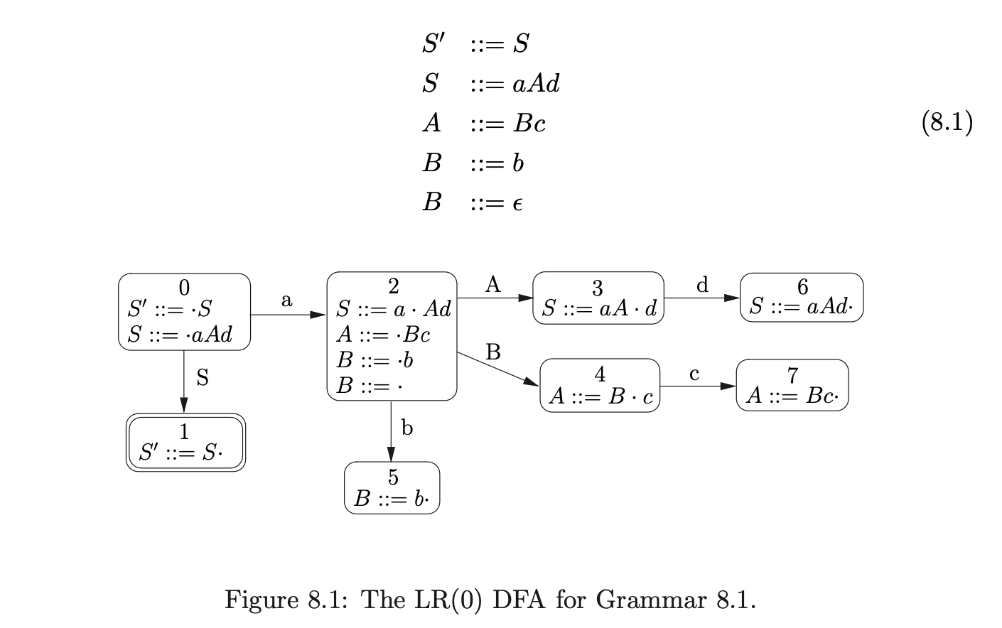
For example, consider Grammar 8.1 and its associated DFA shown in Figure 8.1.

By transforming Grammar 8.1 with the $\epsilon$-removal algorithm, Grammar 8.2 is constructed. For the purpose of clarity, we have used non-terminals of the form $[A]$ to indicate that the non-terminal $A$ has been removed from the grammar by the $\epsilon$-removal transformation.

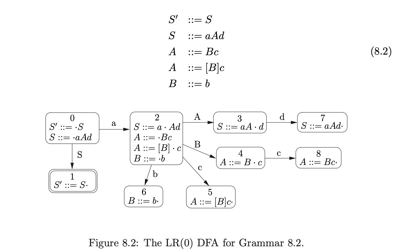
To reduce the number of states in the DFA of a grammar that has had the $\epsilon$-removal transformation applied, we can incorporate the removal of $\epsilon$-rules into the closure function used during the construction of the DFA. We consider rules that are derived from the same basic item to be equivalent. For example, in Figure 8.2 the items $(A::=Bc\cdot)$ and $(A::=[B]c\cdot)$ are considered to be the same and hence states 5 and 7 can be merged and a new edge, labelled $c$, added from state 5.

Although the merging of DFA states in this way can reduce the number of states, it breaks one of the fundamental properties of DFA’s that are used by parsers - if a state that contains a reduction action is reached, then it is guaranteed that the reduction is applicable. As a result, when a reduction is performed by a parser that uses the $\epsilon$-LR DFA, it is necessary to check each of the symbols that are popped off the stack, to ensure that the reduction is applicable at that point of the parse.

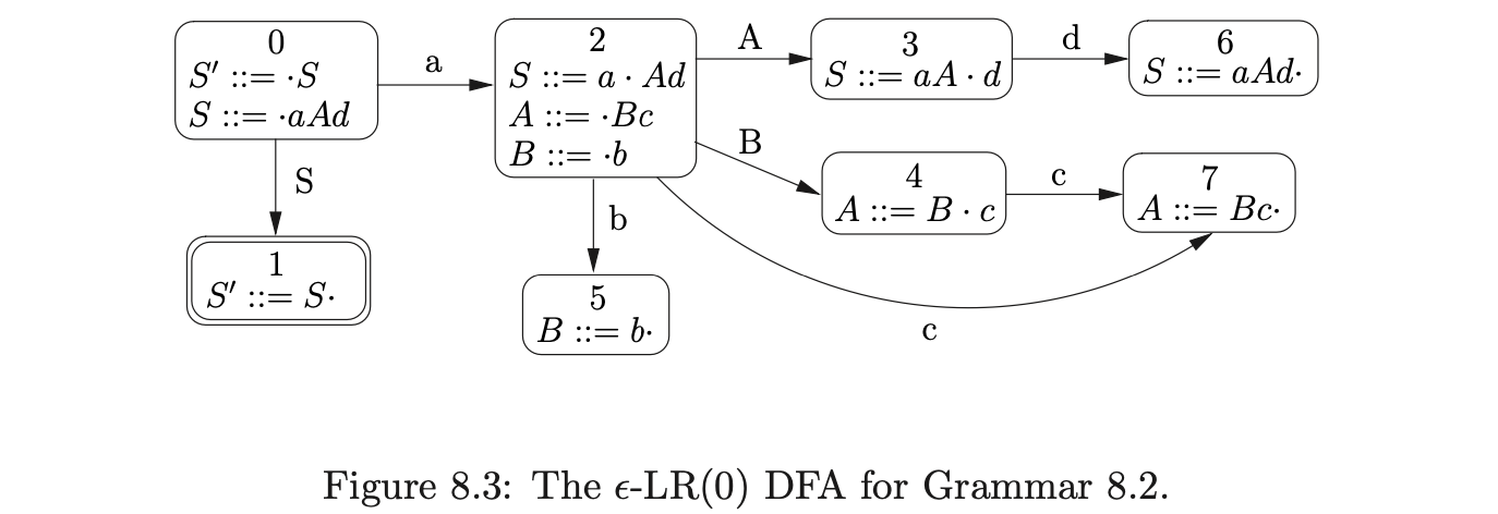
For example, consider the parse of the string $abcd$ using the $\epsilon$-LR(0) DFA in Figure 8.3. We begin by creating the node, $v_{0}$, labelled by the start symbol of the DFA and then perform two consecutive shifts for the first two input symbols $ab$.

From state 5 we can perform a reduce for rule $B::=b$, so we trace back a path of length 1 from $v_{2}$, checking that the symbol on the edge matches the rule, to state $v_{1}$ and create the new node, $v_{3}$ labelled 4.

At this point we can perform the shift on $c$ from state 4 in the DFA to state 7. However, because of the previous reduction the shift is now also applicable from $v_{2}$. We create the new node $v_{4}$ and add edges to both $v_{3}$ and $v_{2}$.

From state 7 there is the reduction, $A::=Bc$. However, recall that state 7 was created by merging states 5 and 8 in the DFA in Figure 8.2, so there are two reductions that are valid at this point. One where $B\Rightarrow\epsilon$ and the other where $B\Rightarrow b$. Therefore we trace back two types of path; one of length 1, where we can pop $c$ off the stack and another of length 2, where we pop $Bc$. Consequently we construct the GSS show below.

Next we can read the final input symbol $d$ and perform the shift from state 3 to state 6. We create the new node $v_{6}$ and create the edge from $v_{6}$ to $v_{5}$.

From state 6 we perform the reduction $S::=aAd$ by tracing back paths of length 3 from $v_{6}$. However, although three different paths can be traversed, ($[v_{6},v_{5},v_{2},v_{1}]$, $[v_{6},v_{5},v_{3},v_{1}]$, $[v_{6},v_{5},v_{1},v_{0}]$) only one is applicable because of the symbols labeling the traversed edges. The final GSS is shown below.

Another solution, which only causes a quadratic increase in the number of rules, is to use the hidden-left recursion removal algorithm. However, a grammar that has been transformed in this way can only be parsed by Tomita’s Algorithm 2, since Algorithm 1 has a problem with right nullable rules. As we shall see in Chapter 10 Algorithm 2 is less efficient than Algorithm 1 (or indeed RNGLR).

8.2 James R. Kipps¶

Tomita’s Algorithm 2 can fail to terminate when parsing strings in hidden-left recursive grammars (see Chapter 4). In [10], Kipps shows that the worst case asymptotic complexity of the algorithm, for grammars without hidden-left recursion, is. However, his proof does not take this into consideration and hence must be incorrect. None of the grammars used in the experimental section of [13] contain hidden-left recursion and hence successfully terminate.

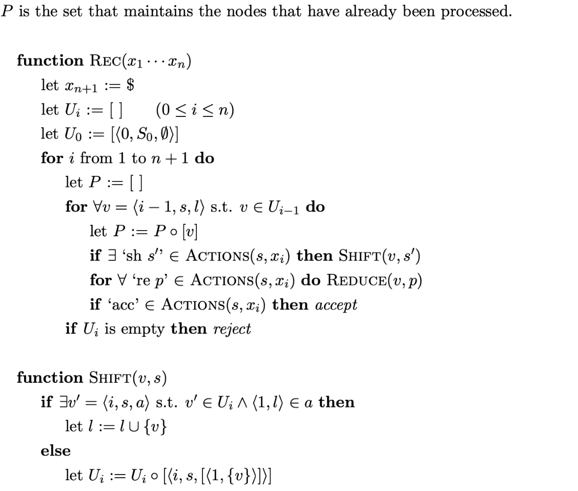
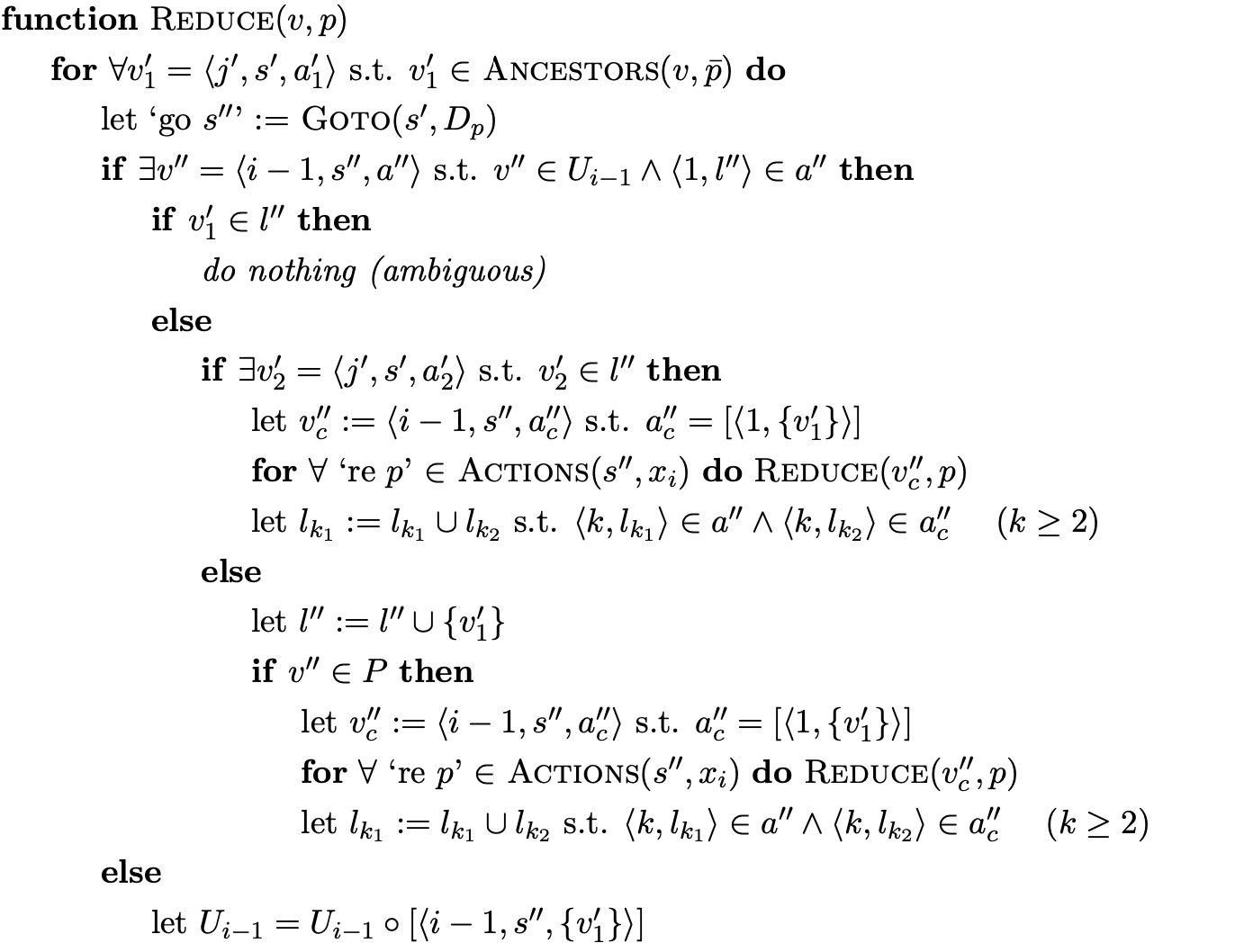
Kipps makes a modification to Tomita’s algorithm which, he claims, makes it achieve worst case time complexity for all context-free grammars. Kipps changes the formal definition used by Tomita in [14]. The Reducer and are combined into one function and the new Ancestors function is used to abstract the search for target nodes of a reduction. Also, instead of defining the algorithm to create sub-frontiers for nullable reductions the concept of a clone vertex is introduced.

Although the notation and layout of the algorithm presented in [13] differs somewhat from Tomita’s Algorithm 2 we believe them to be equivalent. Kipps’ algorithm also fails to terminate on grammars with hidden-left recursion and thus cannot be. The proof that his algorithm is cubic is flawed in the same way that his proof that Tomita’s algorithm is.

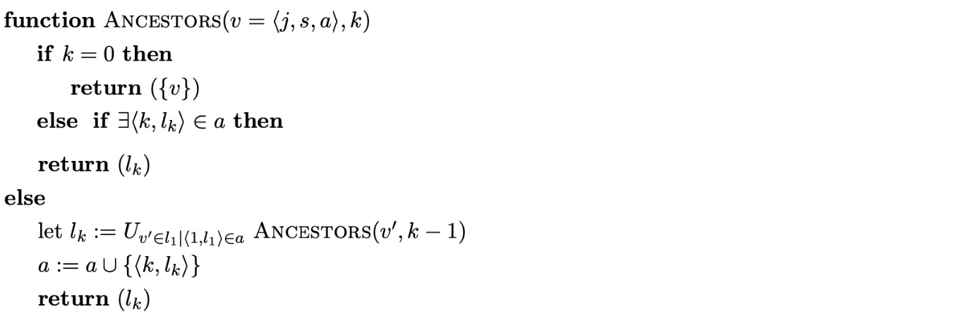
Although Kipps’ proof is flawed the observations on the root of the algorithms complexity are valid - it is the Ancestors function that traces back reduction paths during a reduction that contributes to the complexity of the algorithm. Only the Ancestors function uses steps. However, Ancestors can only ever return at most nodes and there are at most nodes between a node in and its ancestors. So, for steps to be performed in Ancestors some paths must be traversed more than once. Kipps improves the performance of Tomita’s algorithm by constructing an ancestors table that allows the fast look-up of nodes at a distance of.

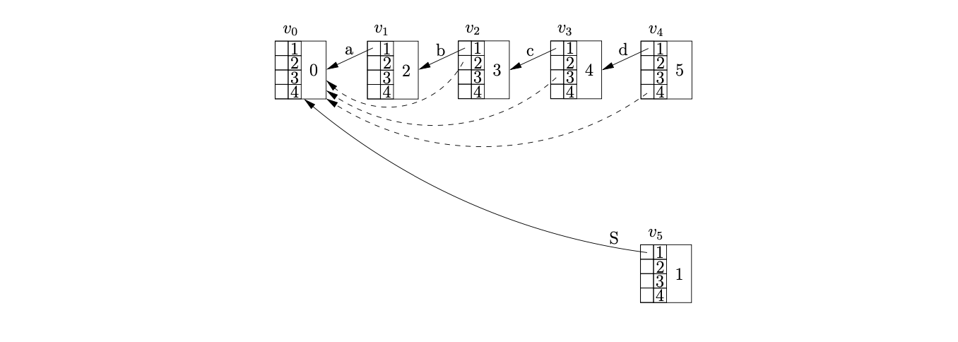
In Kipps’ algorithm a state node is represented as a triple where is the level the state is in, is the state number labeling the node and is the ancestor field that stores the portion of the ancestor table for. In the algorithm the ancestor field of a node consists of sets of tuples where are the set of ancestor (or target) nodes at a length of from node. In our example we draw the GSS nodes with a two dimensional ancestor table, representing the portion of the ancestor table for the node, on the left and the state number on the right. We do not label the level in the node since it is clear by the position of the node. To highlight how the algorithm operates we use dotted arrows for the edges added by the Ancestors function and solid arrows to represent the final edge of a reduction.

The algorithm dynamically generates the ancestor table as reductions are performed.

Before we present the formal specification of Kipps’ algorithm we demonstrate its operation using an example. Recall Grammar 6.5 and its associated DFA in Figure 6.6, shown on page 6.6. To parse the string we begin by creating the new node in. Since there is a shift to state from state on the next input symbol $a$, we create the new node $v_{1}$, labelled 2, in $U_{1}$. We add an entry in the ancestor field of $v_{1}$ to show that $v_{0}$ is an ancestor of $v_{1}$ at a distance of one. We represent this in the diagram by adding an edge from the ancestor table of $v_{1}$ in position 1 to $v_{0}$.

We continue in this way shifting the next three input symbols and creating the nodes $v_{2},v_{3},v_{4}$ labelled 3,4 and 5 respectively.

Processing $v_{4}$ we find a reduce/reduce conflict in state 5 for the current lookahead symbol $\$$. First we perform the reduction on rule $S::=abcd$ by calling the Reducer function. We find the target node of the reduction by calling the Ancestors function. Since there is not a node on a distance of 4 from $v_{4}$, we find node $v_{3}$ at a distance of 1 and call the Ancestors function recursively from $v_{3}$ and a length of three. We repeat the recursion until the length reaches 0 at which point we return the node reached. As the recursion returns to each node on the path between $v_{4}$ and $v_{0}$ we update the ancestor table by adding an edge to the returned target node of the reduction that is getting passed back through the recursion.

The Ancestors function returns $v_{0}$ as the node at a distance of 4 from $v_{4}$. Since no node exists in the frontier of the GSS that is labelled by the goto state of the reduction we create the new node $v_{5}$ with an edge from position one in the ancestor table to $v_{0}$.

We continue by processing the second reduction, $D::=d$, of the reduce/reduce conflict encountered in $v_{4}$. The reduction is of length one and since there is already an edge in the ancestor table of $v_{4}$ the Ancestors function returns $v_{3}$ without performing any recursion. We create the new node $v_{6}$, labelled 6, in $U_{4}$ and add an edge in its ancestor table to $v_{3}$ in position one.

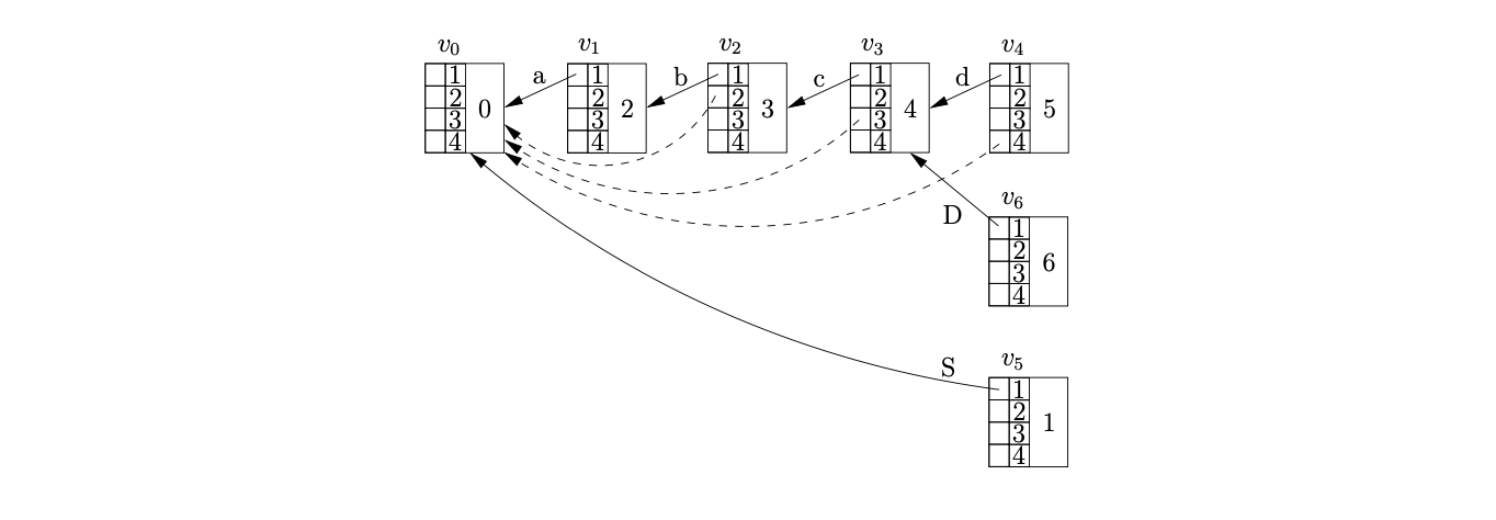
When we process $v_{5}$ we find the accept action in its associated parse table entry. However, since $v_{6}$ has not yet been processed, the termination of the parse is delayed. Processing $v_{6}$ we find the reduction on rule $S::=abcD$. We use the Ancestors function to find the target node of the reduction on a path of length four from $v_{6}$. Since we have already performed a reduction from $v_{4}$ that shares some of the path used by this reduction, the ancestor table in $v_{3}$ contains an edge in position 3 to $v_{0}$. Instead of continuing the recursion, the Ancestors function returns $v_{0}$ as the node at the end of the path of length four from $v_{6}$ without tracing the entire reduction path.

Since $v_{5}$ is labelled by the goto state of the reduction and has an edge to the target node $v_{0}$, the GSS remains unchanged and the parse terminates in success.

Kipps’ $O(n^{3})$ recognition algorithm¶

In a similar way to the BRNGLR algorithm Kipps’ approach trades space for time, but the two algorithms use different techniques to achieve this. In the conclusion of his paper Kipps admits that although his approach produces an asymptotically more efficient parser, the overheads associated with his method do not justify the improvements. He argues that the ambiguity of grammars in real applications is restricted by the fact that humans must be able to understand them.

8.3 Jay Earley¶

One of the most popular generalised parsing algorithms is Earley’s algorithm [1, 1]. First described in 1967, this approach has received a lot of attention over the last 40 years. In this section we briefly discuss the operation of the algorithm and highlight some of its associated problems.

Earley’s algorithm uses a grammar $G$ to parse an input string $X_{1}\ldots X_{n}$ by dynamically constructing sets of items similar to those used by the LR parsing algorithm. The only difference between Earley’s items and the standard LR items used in the DFA construction is the addition of a pointer back to the set containing the base item of the rule.

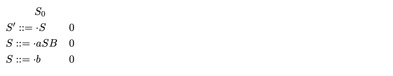
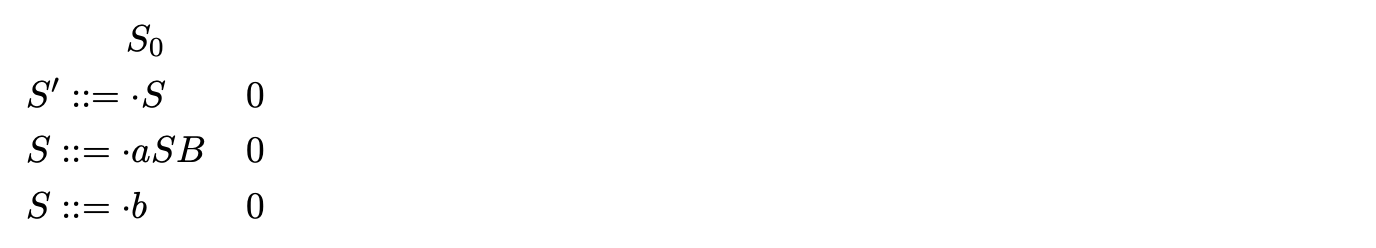
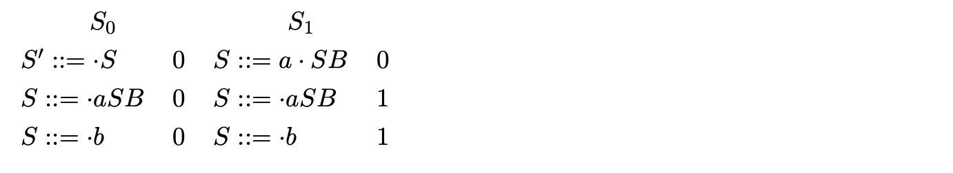
For example consider the parse of the string $aab$ with Grammar 6.1 shown on page 118. We begin by initialising the set $S_{0}$ with the item ($S::=\cdot S\ 0$). We predict the rule for $S$ and add the items ($S::=\cdot aSB\ 0$) and ($S::=\cdot b\ 0$) to $S_{0}$.

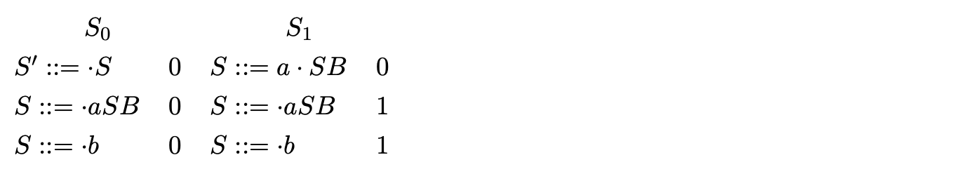
Since no more rules can be predicted we continue by scanning the next input symbol, $a$, and construct the set $S_{1}$ with the item ($S::=a\cdot SB\ 0$). We continue by predicting two more items, ($S::=\cdot aSB\ 1$) and ($S::=\cdot b\ 1$), which completes the construction of $S_{1}$.

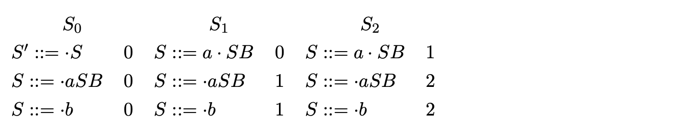
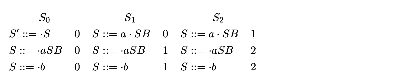
We construct $S_{2}$ by scanning the next input symbol, $a$, adding the item ($S::=a\cdot SB\ 1$) and then predicting two more items ($S::=\cdot aSB\ 2$) and ($S::=\cdot b\ 2$).

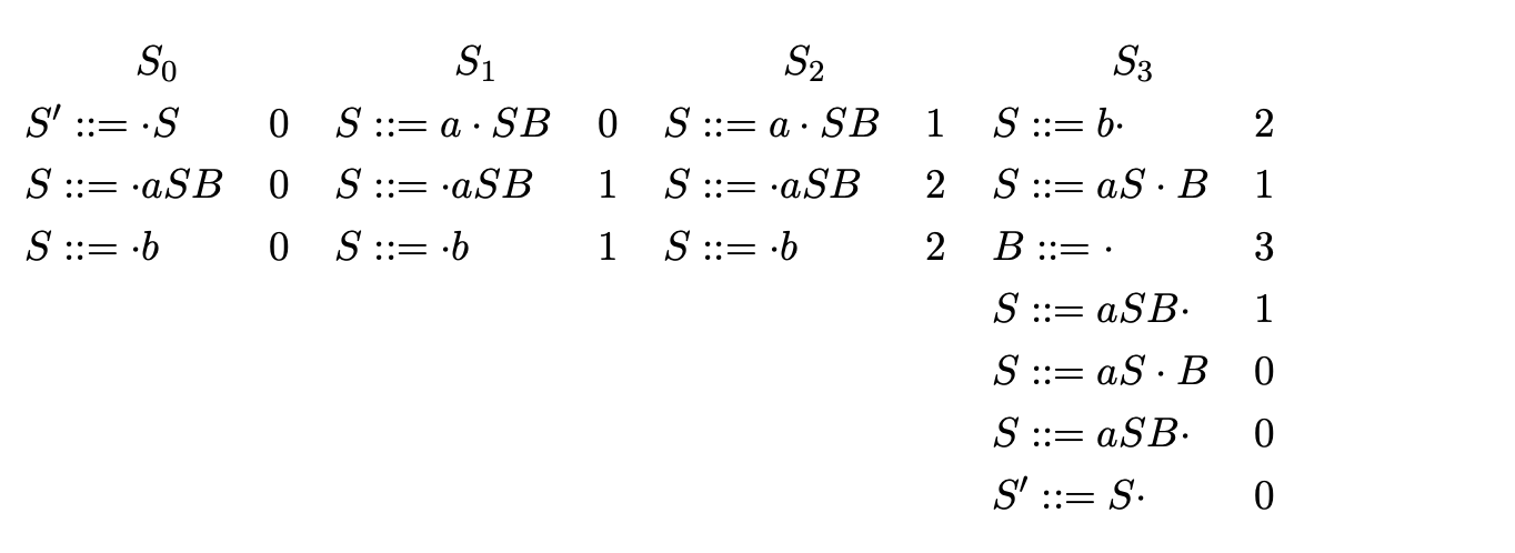
We begin the construction of $S_{3}$ by scanning the symbol $b$ and adding the item ($S::=b\cdot\ 2$). Since the item has the dot at the end of a rule, we go back to the state indicated by the item’s pointer, in this case $S_{2}$, collect all items that have a dot before $S$, move the dot past the symbol and add them to $S_{3}$. In this case only one item is added to $S_{3}$, ($S::=aS\cdot B\ 1$).

We continue by predicting the rule $B::=\epsilon$ and add the item ($B::=\cdot\ 3$). Because the new item added is an $\epsilon$-rule it can be completed immediately. This involves searching over the current state for any items that have the dot before the non-terminal $B$. In this case we find the item ($S::=aS\cdot B\ 1$), which results in the new item ($S::=aSB\cdot\ 1$) being added to the current state. We then complete this item by going back to $S_{1}$ and finding the item ($S::=a\cdot SB\ 0$) which we then add to $S_{3}$ as ($S::=aS\cdot B\ 0$).

Normally at this point we predict the item ($B::=\epsilon$). However, since the item already exists in the current state, we do not add it again to prevent the algorithm from not terminating on left recursive grammars. Instead we perform the any completions that have not already been performed in the current state for the non-terminal $B$. This results in the addition of the item ($S::=aSB\cdot\ 0$) which in turn causes the item ($S^{\prime}::=S\cdot\ 0$) to be added to $S_{3}$.

Since no more rules can be predicted we continue by scanning the next input symbol, a, and construct the set $S_{1}$ with the item $(S::=a \cdot S B 0)$. We continue by predicting two more items, $(S:=\cdot a S B 1)$ and $(S::=\cdot b 1)$, which completes the construction of $S_{1}$.

We construct $S_{2}$ by scanning the next input symbol, a, adding the item ( $S:= a \cdot S B 1$) and then predicting two more items ($S::=\cdot aSB2$) and ($S::=\cdot b 2$). We begin the construction of $S_{3}$ by scanning the symbol b and adding the item ($S::=b \cdot 2$). Since the item has the dot at the end of a rule, we go back to the state indicated by the item’s pointer, in this case $S_{2}$, collect all items that have a dot before S, move the dot past the symbol and add them to $S_{3}$. In this case only one item is added to $S_{3}$,($S::=a S \cdot B 1$). We continue by predicting the rule $B::=\epsilon$ and add the item ($B::=\cdot 3$). Because the new item added is an $\epsilon-rule$ it can be completed immediately. This involves searching over the current state for any items that have the dot before the nonterminal B. In this case we find the item ($S::=a S \cdot B 1$), which results in the new item ($S::=a S B \cdot 1$) being added to the current state. We then complete this item by going back to $S_{1}$ and finding the item ($S::=a \cdot S B 0$) which we then add to $S_{3}$ as ($S:=a S \cdot B 0$). Normally at this point we predict the item ($B::=\epsilon$). However, since the item already exists in the current state, we do not add it again to prevent the algorithm from not terminating on left recursive grammars. Instead we perform the any completions that have not already been performed in the current state for the non-terminal B. This results in the addition of the item (S::=a S B \cdot 0) which in turn causes the item $\left(S^{\prime}::=S \cdot 0\right)$ to be added to $S_{3}$.

At this point no more items can be created and since we have consumed all the input and the item ($S^{\prime}::=S\cdot\ 0$) is in the final state, the parse terminates in success. Each item consists of a grammar rule with a dot on its right hand side, a pointer back to the set where we started searching for a derivation using this rule and a lookahead symbol. The dotted rule is that represents the part of the rule that has been used to recognise a portion of the input string,Instead of pre-constructing a DFA for $G$, the algorithm constructs the state sets on-the-fly. This avoids the need of a stack during a parse. As each input symbol is parsed a new set of items is constructed which represents the rules of the grammar that can be reached after reading the input string. Instead of pre-constructing a DFA for G, the algorithm constructs the state sets on-the-fly. This avoids the need of a stack during a parse. As each input symbol is parsed a new set of items is constructed which represents the rules of the grammar that can be reached after reading the input string.

Earley’s algorithm¶

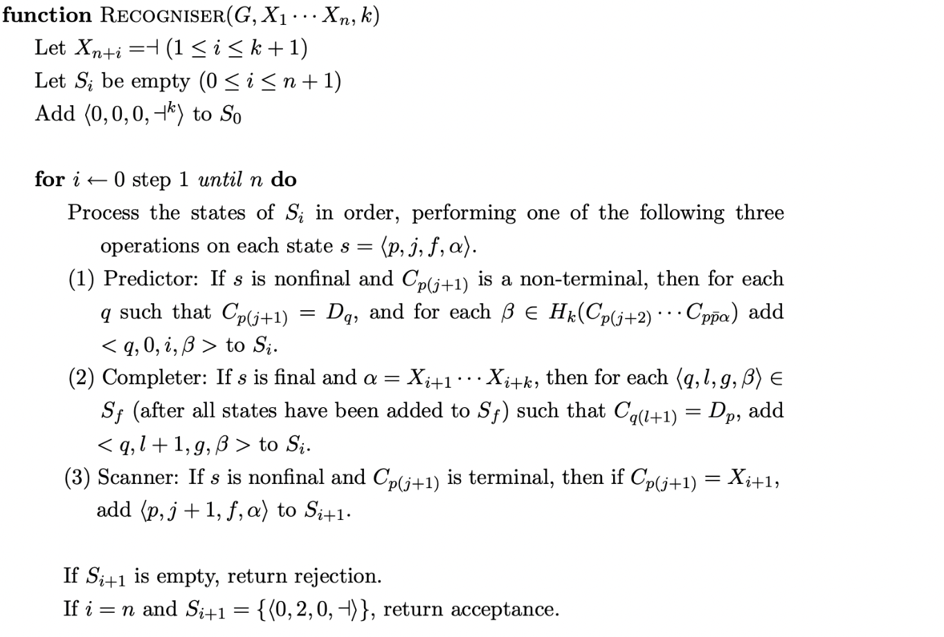
Earley’s algorithm accepts as input a grammar $G$ and a string is $X_{1}\ldots X_{n}$. The grammar productions need to be numbered from $1,\ldots,d-1$ and the grammar should be augmented, with the augmented rule numbered $0$. The $\dashv$ symbol is the end of string terminator instead of $\$$.

A state is defined as a four tuple $\langle p,j,f,\alpha\rangle$, where $p$ is a production number, $j$ position in the rule, $f$ is the number of the state set $S_{f}$ that the item has been constructed from and $\alpha$ is the lookahead used.

The state set acts as a queue where every element is added to the end of the set unless it is already a member of the set.

In addition to some data structures used to achieve the required time and space bounds extra searching needs to be done in the case of grammars containing $\epsilon$-rules. When an $\epsilon$ reduction, $A::=\cdot$ is encountered within a state set $S_{i}$ it is necessary to go through the set $S_{i}$ and move on any of the items with a dot before the nonterminal $A$. This must be done cautiously as some of the items that require the move may not have been created yet. It is therefore necessary to check if this reduction is possible when new items are added to the set.

The formal specification of Earley’s algorithm shown below is taken from [1]. It is this algorithm that has been implemented and used to compare the performance between the RNGLR and BRNGLR algorithms in Chapter 10.

Earley’s algorithm is described as a depth-first top-down parser with bottom-up recognition [1]. In Chapter 2 we discussed how a non-deterministic parse can be performed by using a depth-first search to find a successful derivation, but decided that such an approach is infeasible for practical parsers because of the possible exponential time complexity required. Earley’s algorithm restricts the amount of searching that is required by incorporating bottom-up style reductions in his algorithm.

The description given by Earley in his thesis constructs lists of items, however Graham [1] describes Earley’s algorithm using a recognition matrix, where the item $(A::=\alpha\cdot\beta,i)$ is in the $(i,j)$th entry. This is done to allow a comparison between the CYK and Earley algorithms.

Earley’s algorithm is often preferred to the CYK algorithm for two main reasons; the grammar does not need to be in any special form and the worst case time and space bounds are not always realised. In fact the algorithm is quadratic on all unambiguous grammars and linear on a large class of grammars which include the bounded state grammars and most LR(k) grammars (excluding some right recursive grammars). However, those LR(k) grammars that are not bounded state can be parsed in linear time if extra lookahead is used. (Note that the lookahead is not needed for the $n^{3}$ and $n^{2}$ bounds to be realised.)

Earley claims that the recogniser can be easily extended to a parser without affecting the time bounds, but increasing the space bound to $n^{3}$, because of the need to store the parse trees. However, the extension presented in [1] has been shown to create spurious derivations for some parses [16].

Earley also says that his algorithm has a large constant coefficient and when compared to the linear techniques does not compare well. This is because the linear parsers usually compile a parser for a given grammar and use it to parse the input without needing to refer to the grammar. A pre-compiled version of the algorithm is presented in [1] but does not work for all grammars. In fact it is shown that determining whether a given grammar is compilable is undecidable and they cannot even be enumerated. Others [1, 10, 11, 12] have attempted to improve the performance of Earley’s algorithm with the use of a pre-compiled table. We only know of one publication [1] that reports an implementation and experimental results of this approach.

It is uncertain how the use of lookahead affects the algorithm’s efficiency. Earleystates that the $n^{3}$ and $n^{2}$ time bounds can be achieved without lookahead but $k$ symbols of lookahead are required for the algorithm to be linear on LR(k) grammars. It is shown that the number of items in a set can grow indefinitely if lookahead is not used to restrict which items are added by the Completer step. It was later shown by [1] that a better approach is to use the lookahead in the Predictor step instead.

Earley’s algorithm has been implemented essentially as written above in PAT and results of the comparison with the BRNGLR algorithm are given in Chapter 10.

8.4 Bernard Lang¶

Lang developed a general formalism to resolve non-deterministic conflicts in a bottom-up automaton by performing a breadth first search. Tomita’s GLR parsing algorithm can be seen as a realisation of Lang’s ideas. Unfortunately, due to the complex description of his algorithm, Lang’s approach is often overlooked. In this section we discuss the main properties of Lang’s algorithm.

Lang’s work is an efficient breadth first search approach to dealing with non-determinism in a bottom-up automaton (PDT). Earley’s algorithm is a general top-down parsing algorithm and Lang develops a bottom-up equivalent. The algorithm also outputs a context-free grammar whose language is the derivations of a sentence.

Lang uses a PDT and an algorithm $\mathcal{G}$ to calculate all the possible derivations for a sentence $d$ of length $n$. $\mathcal{G}$ successively builds $n+1$item sets while parsing the input. Each item set $\mathcal{S}_{i}$ contains the items that are reached after parsing the first $i$ symbols of $d$. Each item takes the form $((p,A,i),(q,B,j))$ where $p$ and $q$ are state numbers; $A$ and $B$ are non-terminals; $i$ and $j$ are indexes into the input. The algorithm $\mathcal{G}$ uses old items and the PDT transitions to build the new items.

Lang’s algorithm is cubic because the PDT only allows one symbol to be popped off the stack in one action. This means that his algorithm does not apply to the natural LR automaton unless either his algorithm or the automaton is modified, or the grammar’s rules have a maximum length of two [15]. Modifying the automaton significantly increases its size (the number of actions needed). If Lang’s algorithm is modified to allow more than one symbol to be popped off the stack in one action the complexity changes to $O(n^{k})$.

8.5 Klaas Sikkel¶

Klaas Sikkel’s book on parsing schemata [14] presents a framework capable of comparing different parsing techniques by abstracting away “algorithmic properties such as data structures or control mechanisms”. This framework allows the comparison of different algorithms in a way that facilitates cross fertilisation of ideas across the techniques. This is clearly an important approach, although somewhat more general than the specific goal of this thesis. In particular, parsing schemata are used to examine the similarity of Tomita’s and Earley’s algorithms.

As part of the analysis undertaken in [22], there is a detailed discussion of Tomita’s approach and a description of a parallel bottom-up Tomita parser. The algorithm described is Algorithm 2 and included is a discussion of Kipps’ proof that this algorithm is worst case $O(n^{k+1})$. This proof, like Kipps’ original, is based on Tomita’s Algorithm 1 and ignores the sub-frontiers introduced in Algorithm 2. This is a proof that Algorithm 1 has worst case time complexity $O(n^{k+1})$.