5. Right Nulled Generalised LR parsing
Tomita’s Algorithm 1 can fail to terminate when parsing strings in the language of grammars with hidden-right recursion and Algorithm 2 can fail on grammars with hidden-left recursion. In Chapter 4 we considered Farshi’s extension to Tomita’s Algorithm 1 that increases the searching required during the construction of the GSS, but which is able to parse all context-free grammars. This chapter presents an algorithm capable of parsing all context-free grammars without the increase in searching costs.
It is clear that Tomita was aware of the problems associated with Algorithm 1 as he restricted its use to \(\epsilon\)-free grammars. It is not unusual to exclude \(\epsilon\)-rules from parsing algorithms as difficulties are often caused by them; for instance the CYK algorithm requires grammars to be in Chomsky Normal Form. One of the reasons for using \(\epsilon\) in grammars is that many languages can be defined naturally using \(\epsilon\)-rules while the \(\epsilon\)-free alternatives are often less compact and not as intuitive. Well known alg orithms exist [1] that can remove \(\epsilon\) from grammars, but parsers that depend on this technique build parse trees related to the modified grammar. Another approach [13] that performs automatic removal of \(\epsilon\)-rules during a parse is discussed in Chapter 8.
This chapter presents a modification to the LR DFA’s that allow Tomita’s Algorithm 1 to parse all context-free grammars including those with \(\epsilon\)-rules. We discuss Algorithm 1 on \(\epsilon\)-rules in detail and examine some grammars that cause the parser to fail. A modification to the parse table is then given that causes the algorithm to work correctly. The RNGLR algorithm that parses strings using the modified parse table more efficiently than Algorithm 1 on \(\epsilon\)-rules is then presented both as a recogniser and then as a parser. Finally, we discuss ways to reduce the extra non-determinism introduced by the modification made to the parse table.
5.1 Tomita’s Algorithm 1e
Algorithm 1 provides a clear exposition of Tomita’s ideas. Unfortunately it cannot be used to parse natural language grammars as they often contain \(\epsilon\)-rules. Tomita’s Algorithm 2 includes a complicated procedure for dealing with \(\epsilon\)-rules which fails to terminate on grammars containing hidden-left recursion. The algorithm below, which we have called Algorithm 1e, is a straightforward extension to Algorithm 1 to include \(\epsilon\)-rules, which works correctly for hidden-left recursive grammars, but may fail on grammars with hidden-right recursion. We begin this section by describing the modifications made to Algorithm 1 to allow \(\epsilon\)-rules to be handled.
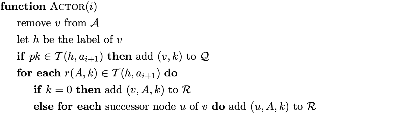
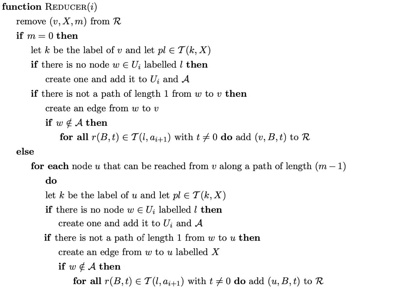
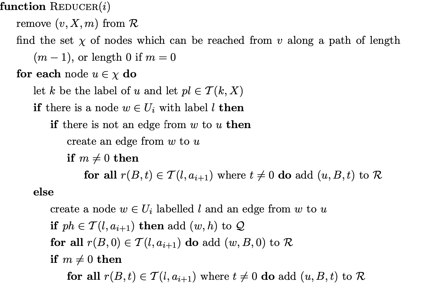
It is straight-forward to modify Tomita’s Algorithm 1 so that it can handle grammars containing \(\epsilon\)-rules. The two main changes that need to be made are in the Actor and Reducer functions. When an \(\epsilon\) reduce action \(rX\) from a state \(v\) is found by the Actor, \((v,X)\) is added to \(\mathcal{R}\) instead of \((u,X)\), where \(u\) are the successors of \(v\). Since \(\epsilon\) reductions do not require any states to be popped off the stack, no reduction paths are traced in the Reducer.
It has already been shown, in Chapter 4, that it is possible to add a new edge to an existing state in the current level of the GSS. In this case the reductions from the existing state need to be applied down the newly created reduction path. However, not all reductions need to be re-done. Since \(\epsilon\) reductions do not pop any states off the stack, no new reduction path is added by the addition of the new edge. Because we store all pending reductions in the set \(\mathcal{R}\), and all \(\epsilon\) reductions are added to it when a new state is created, we can safely assume that if the \(\epsilon\) reductions have not already been done, they eventually will. Therefore no \(\epsilon\) reductions are added to \(\mathcal{R}\) when a new edge is added to an existing state. This modification was added to Tomita’s Algorithm 3, and since we have extended Algorithm 1 to allow \(\epsilon\) grammars to be parsed we have included this modification to Algorithm 1e as well.
Tomita’s original algorithms build GSS’s with symbol nodes between state nodes. Algorithm 1e does not include the symbol nodes, but in our diagrams we shall label the edges to make the GSS’s easier to visualise. As we shall see in Section 5.5 this approach also allows more compact SPPF’s to be generated.
To allow a closer comparison to the algorithms we introduce later we have changed the layout of Algorithm 1e and the format of the actions in the parse table: instead of using \(sk\) and \(gk\) to represent the shift and goto actions, we use \(pk\) for both; instead of using \(rj\) to represent a reduction on rule \(j\), we use \(r(X,m)\) where \(X\) is the left hand non-terminal of rule \(j\) and \(m\) is the length of \(j\)’s right hand side.
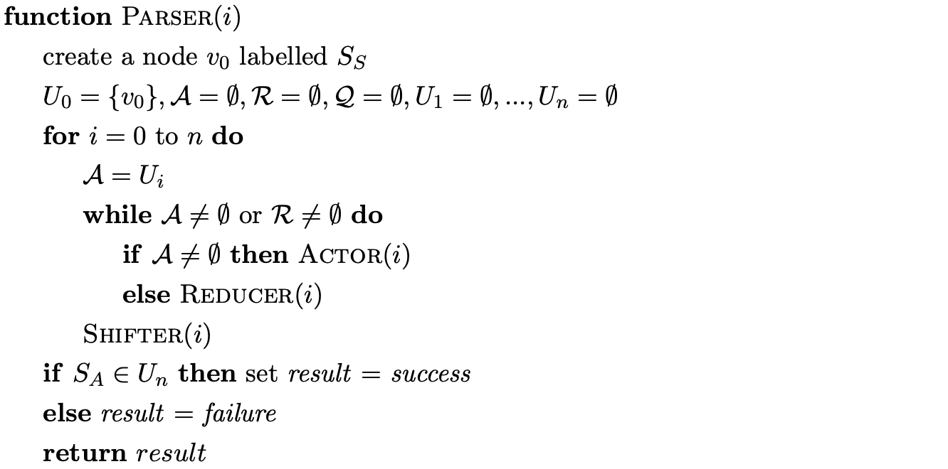
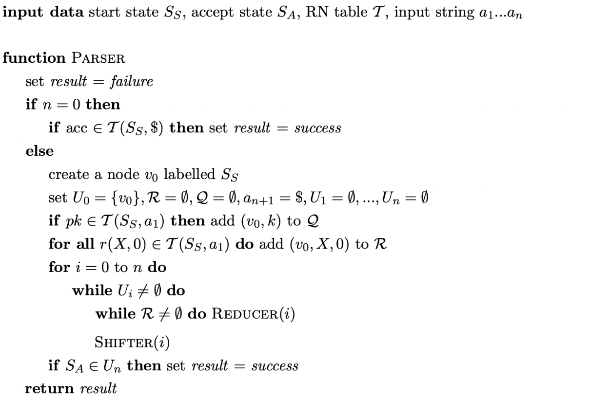
Algorithm 1e
input data start state \(S_{S}\), accept state \(S_{A}\), parse table \(\mathcal{T}\), input string \(a_{1}...a_{n}\)


5.1.2 Paths in the GSS
Algorithm 1 ensures that a reduction is only applied down a certain reduction path once. This is achieved by queueing the first edge of the path and the associated rule of the reduction in the set \(\mathcal{R}\) when a new edge is created in the GSS. If a new edge is added to an existing node, any applicable reductions are applied down this new reduction path. For this approach to be successful it is essential that the new edge cannot be added to the middle of an existing reduction path. This is achieved by Algorithm 1 since all new edges created have their source node in the frontier and their target in a previous level of the GSS. However, the modification of Algorithm 1e to deal with \(\epsilon\)-rules allows edges to be created whose source and target nodes are in the same level. As a result of this, certain grammars can cause a new edge to be added to the middle of an existing reduction path. We illustrate this with the following example.
Example - an incorrect parse
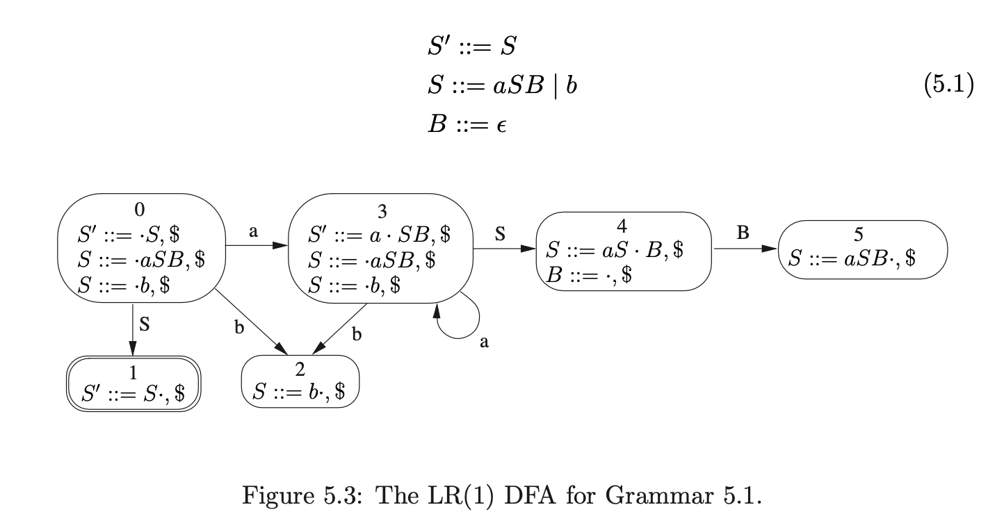
Consider Grammar 5.1 and the associated LR(1) DFA in Figure 5.3 (previously encountered on page 5.1).
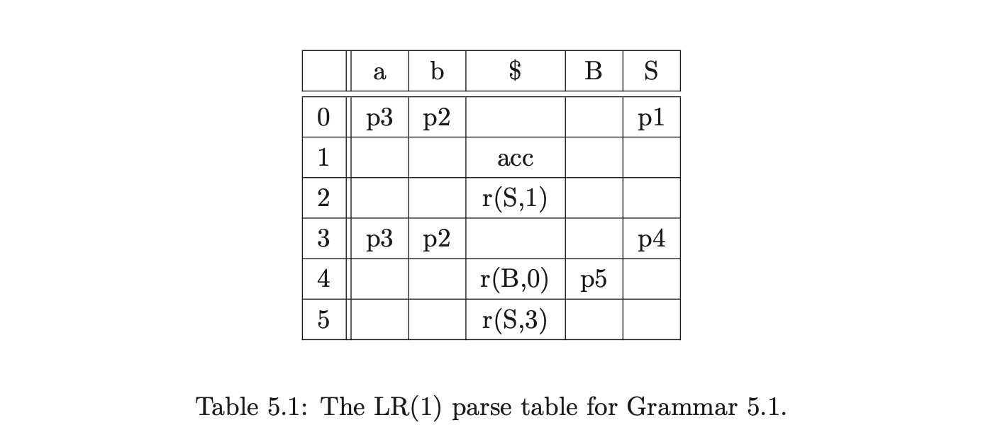
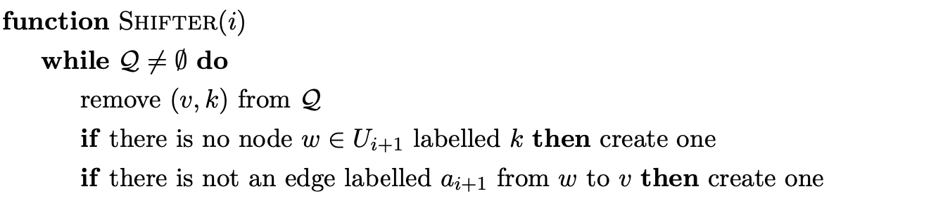
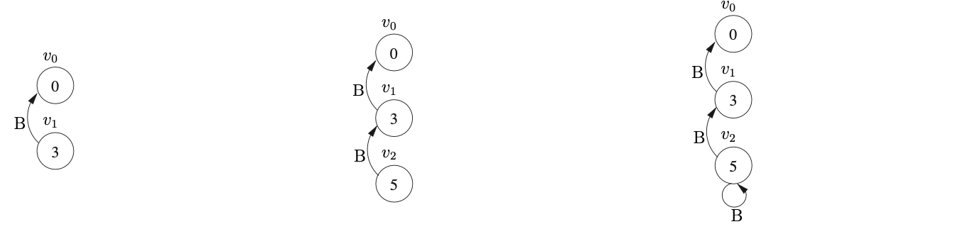
We shall use Algorithm 1e to construct the GSS for the string \(aab\). We begin by creating the start state, \(v_{0}\), in \(U_{0}\) and look up the actions in \(\mathcal{T}(0,a)\). As there is only a shift to state 3, \((v_{0},3)\) is added to \(\mathcal{Q}\) and ultimately results in state \(v_{1}\), and the edge \((v_{1},v_{0})\) being created in \(U_{1}\). The Actor then processes \(v_{1}\) and adds \((v_{1},3)\) to \(\mathcal{Q}\).
This results in a new state labelled 3 being created in \(U_{2}\) and the edge \((v_{2},v_{1})\) being added to the GSS. After processing \(v_{2}\) the state \(v_{3}\) labelled 2 and the edge \((v_{3},v_{2})\) is created.

When the Actor processes \(v_{3}\) it finds a reduce action in \(\mathcal{T}(2,\$)\) which it adds to the set \(\mathcal{R}\) as \((v_{2},2)\). The Reducer then removes \((v_{2},2)\) and creates the state \(v_{4}\) labelled 4 and the edge \((v_{4},v_{2})\). Processing \(v_{4}\) results in \((v_{4},3)\) being added to \(\mathcal{R}\) which leads to the new state \(v_{5}\) labelled 5 and the edge \((v_{5},v_{4})\) labelled B being added to \(U_{3}\).
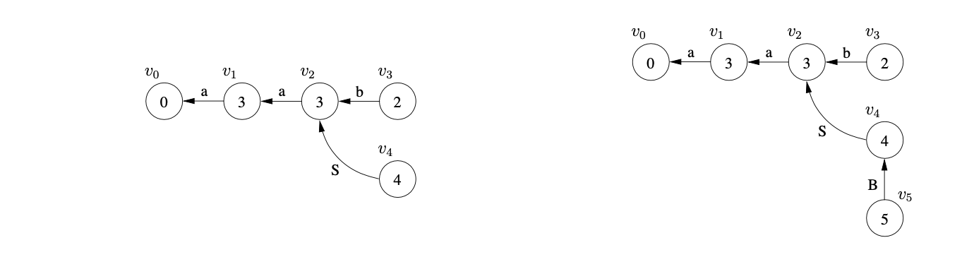
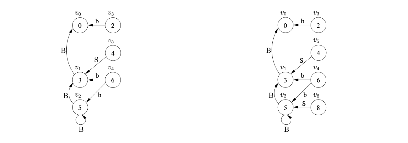
When the new state \(v_{5}\) is processed a reduce action is found in \(\mathcal{T}(5,\$)\) which is added to \(\mathcal{R}\) as \((v_{4},1)\). This reduction is traced back to \(v_{1}\) whose goto state is 4. As a state already exists in \(U_{3}\) labelled 4, a new edge \((v_{4},v_{1})\) labelled S is added to the GSS. Because a new edge is added to an existing node, the reduction from \(v_{4}\) is re-done, but as there is already a state labelled 5 and an edge \((v_{5},v_{4})\) in the current level, nothing is done.
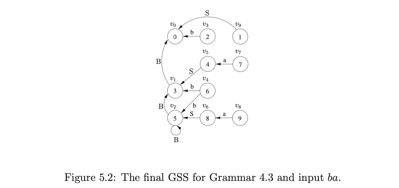
At this point all the sets are empty so \(U_{3}\) is searched for the accept state, which is labelled 1. As no state labelled 1 exists in \(U_{3}\) Algorithm 1e returns false as the result to the parse even though \(aab\) is in the language of Grammar 4.2.

It turns out that some grammars with right nullable rules (rules of the form \(A::=\alpha\beta\) where \(\beta\stackrel{{*}}{{\Rightarrow}}\epsilon\)) can be successfully parsed by Algorithm 1e when the ordering of reductions is carefully chosen. However, grammars such as 4.2 that contain hidden-right recursion will always fail to parse some sentences in their language [15].
The next section presents a modification that can be made to the parse table, which will enable Algorithm 1e to correctly parse all context-free grammars.
5.2 Right Nulled parse tables
In order to allow Algorithm 1e to correctly parse all context-free grammars, a slightly modified parse table is built from the standard DFA in the following way. In addition to the standard reductions, we add reductions on right nullable rules, that is rules of the form \(A::=\alpha\beta\) where \(\beta\stackrel{{*}}{{\Rightarrow}}\epsilon\).
If the DFA has a transition from state \(h\) to state \(k\) on the symbol \(a\) then \(pk\) is added to \(\mathcal{T}(h,a)\) instead of \(sk\) or \(gk\) if \(a\) is a terminal or non-terminal respectively. If state \(h\) includes an item of the form \((A::=x_{1}\ldots x_{m}\cdot B_{1}\ldots B_{t},a)\) where \(A\neq S^{\prime}\) and \(t=0\) or \(B_{j}\stackrel{{*}}{{\Rightarrow}}\epsilon\) for all \(0\leq j\leq t\), then \(r(A,m)\) is added to \(\mathcal{T}(h,a)\). If state \(h\) contains an item \((S^{\prime}::=S\cdot,\$)\) then \(acc\) is added to \(\mathcal{T}(h,\$)\) and if \(S^{\prime}\stackrel{{*}}{{\Rightarrow}}\epsilon\) then \(acc\) is also added to \(\mathcal{T}(0,\$)\). We call this type of parse table a Right Nulled (RN) parse table.
Our approach takes advantage of the fact that no input is consumed when an \(\epsilon\) is parsed. By performing the part of the right nullable reduction that does derive a portion of the input string we ensure that no new edges can be added to the middle of an existing reduction path. Clearly this prevents a reduction path being missed by a state in the sequence of nullable reductions.
It is possible to think that because nullable reductions do not consume any input it is safe not to apply them at all. Unfortunately this can cause problems which are discussed in detail in Section 5.3.
We note here that there are other parsing optimisations, such as [1], that have been proposed that require \(\epsilon\) reductions to be taken account of at parser generation time. So if an item \(A::=\alpha\cdot B\beta\in U_{i}\) and \(B\stackrel{{*}}{{\Rightarrow}}\epsilon\) the item \(A::=\alpha B\cdot\beta\) is added to \(U_{i}\). This is not the same as the right nullable reductions in RN parse tables.
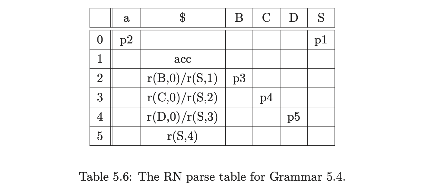
Although the RN parse table enables Algorithm 1e to work correctly for all context-free grammars, see [11] for a proof of correctness, it contains more conflicts than its LR(1) counterpart. The next section presents a method to remove many of these conflicts introduced by the addition of right nullable reductions.
5.3 Reducing non-determinism
An undesirable side effect caused by the inclusion of the right nulled reductions in the RN parse table is a possible increase of non-determinism. As more reductions are added, it is possible that more reduce/reduce conflicts will occur (see Chapter 10).
Since our technique for correctly parsing hidden-right recursive grammars involves performing nullable reductions at the earliest point possible, one may hypothesise that the short circuited \(\epsilon\) reductions can be removed from the table to reduce the non-determinism. Unfortunately this is not always possible because \(\epsilon\) reductions may also include other useful derivations that do consume some input symbols.
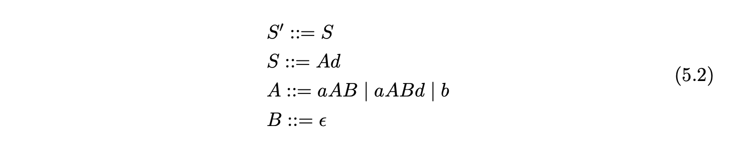
For example, consider Grammar 5.2, the corresponding DFA in Figure 5.4 and the RN parse table 5.3.
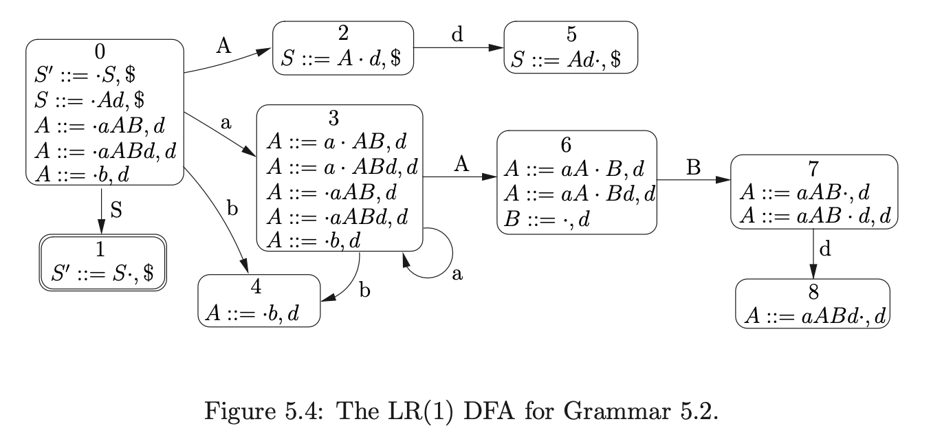
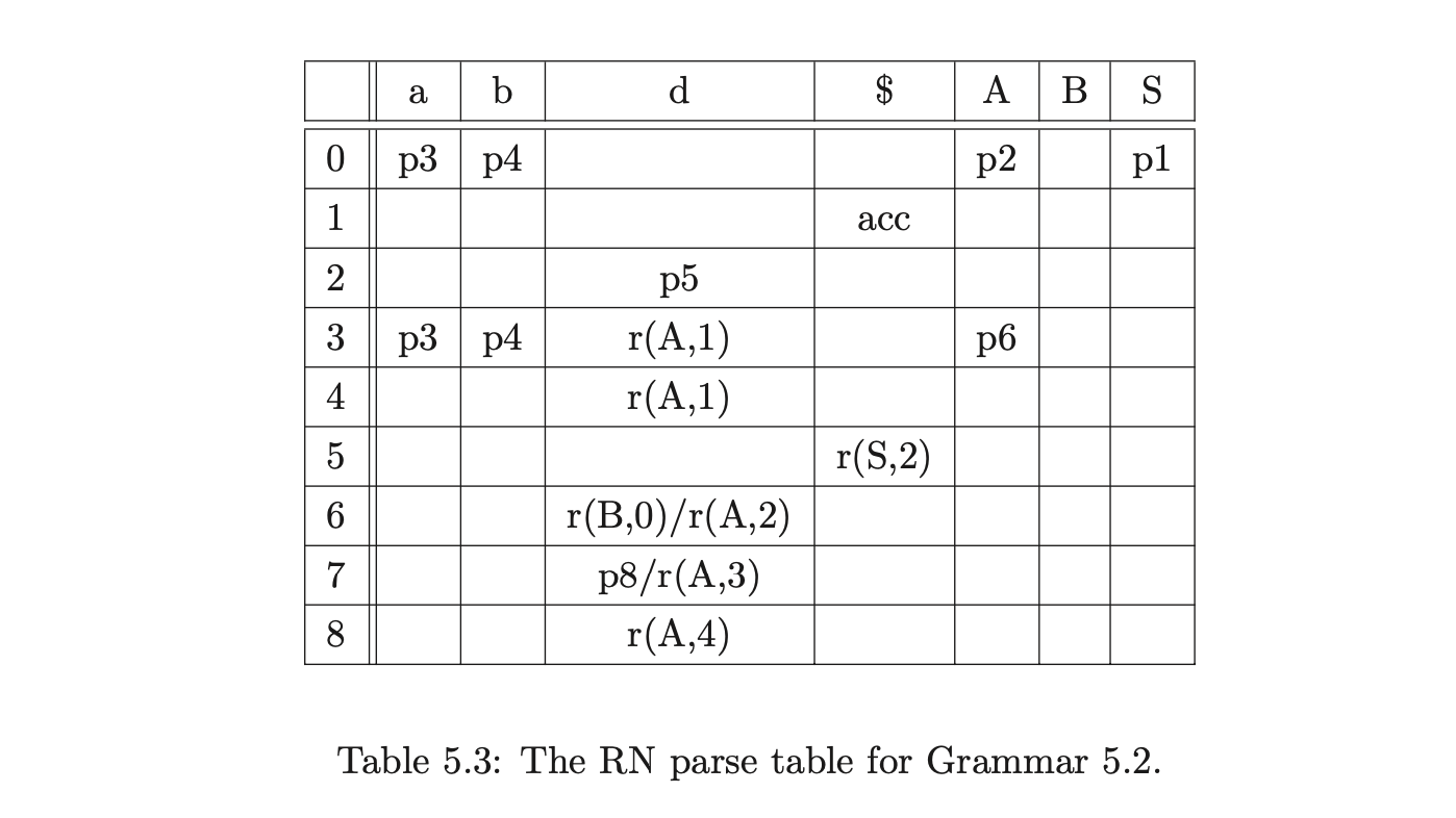
The LR(1) parse table is already non-deterministic, but the number of conflicts is increased when the RN reduction \(r(A,2)\) is added to state 6. This will result in an increase in the amount of graph searching performed for certain parses such as the string \(aabd\). Although the extra searching can be avoided by removing the \(\epsilon\) reduction \(r(B,0)\) from state 6, there are some strings that Algorithm 1 would then incorrectly fail to parse. For example, consider the parse of the string \(aabdd\) using parse table 5.3 and Algorithm 1.
Once we have parsed the first three input symbols and performed the reduction \(r(A,1)\) from state \(v_{3}\) we have the following GSS.

Performing the RN reduction \(r(A,2)\) from state \(v_{4}\) causes the new edge between \(v_{4}\) and \(v_{1}\) to be created. This new edge introduces a new reduction path from \(v_{4}\) to \(v_{0}\), so we create \(v_{5}\) and add an edge between it and \(v_{0}\).

From state 2 there is a shift to state 5, so we create the new state node \(v_{7}\) and the edge between \(v_{7}\) and \(v_{5}\).

By not performing the \(\epsilon\) reduction from state 6 we avoid some redundant graph searching, but for this parse, we also incorrectly reject a string in the language of Grammar 5.2.
Although it is not generally possible to remove \(\epsilon\) reductions from the parse table it is possible to identify points in the GSS construction when their application is redundant. The next section presents a general parsing algorithm, based on Algorithm 1e, that incorporates this allowing right nullable grammars to be parsed more efficiently. In Section 5.6 we discuss an approach that eliminates redundant reductions without compromising the correctness of the underlying parser for RN parse tables of LR grammars.
5.4 The RNGLR recognition algorithm
This section presents the Right Nulled GLR (RNGLR) recogniser which correctly parses all context-free grammars with the use of an RN parse table [15]. A description of the algorithm is given and a discussion highlighting the differences between RNGLR and Algorithm 1e is undertaken.
RNGLR recogniser
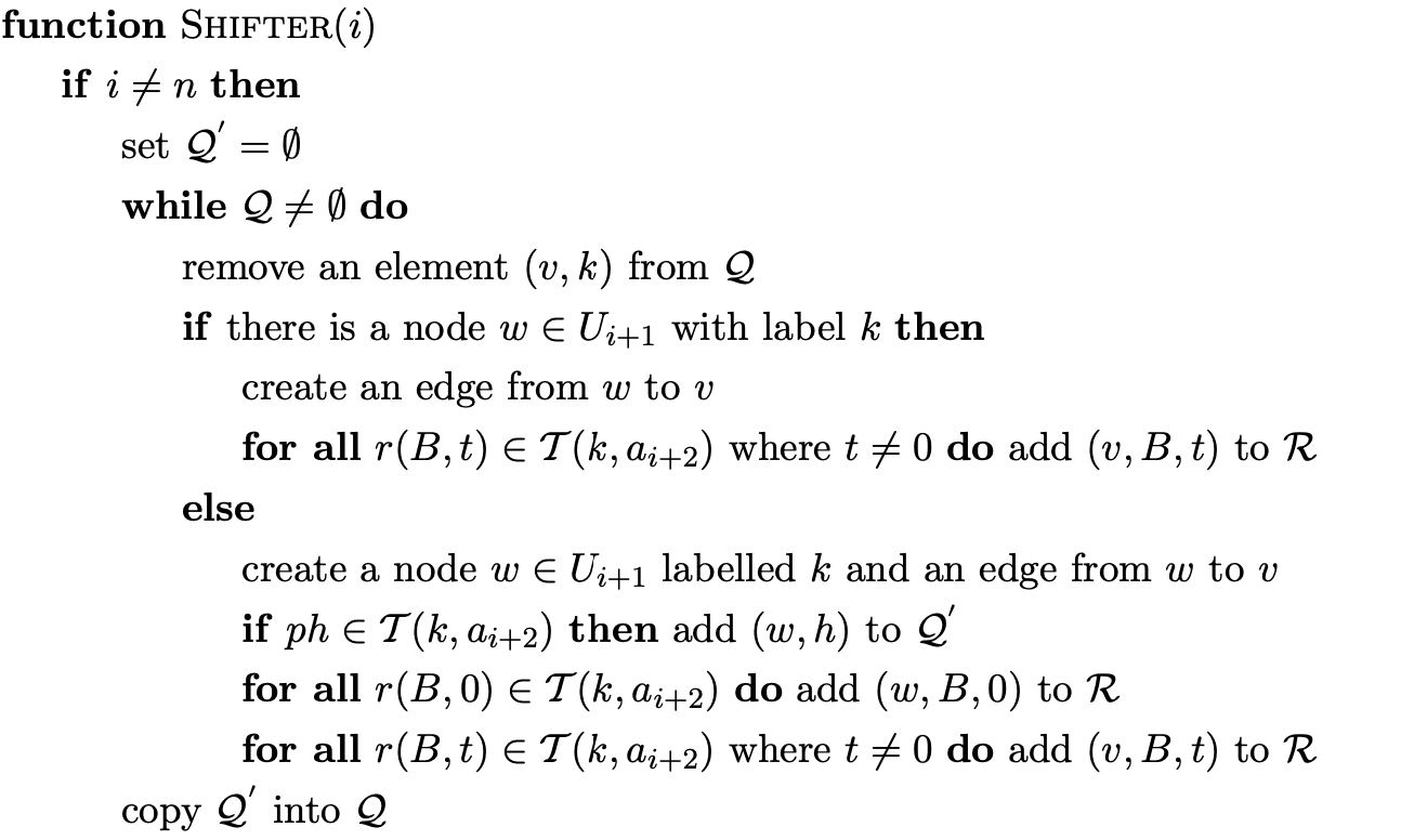
The RNGLR algorithm looks very similar to Algorithm 1e but includes some subtle changes that make a big difference to the efficiency of the algorithm. One of the major differences in the appearance between the two algorithms is the lack of the Actor function in RNGLR. When a new node is created in the GSS by Algorithm 1e the Actor is used to perform the parse table lookup to retrieve the actions associated to the state that labels the new node. If a reduction of length \(>0\) is found then the Actor finds the new node’s successors and adds the triple \(\langle v,x,p\rangle\) to the set \(\mathcal{R}\). The reason for using the successors of a new node is to ensure that when a reduction is done, it is only performed down the same path at most once. However, the successor nodes are known when a new node is created by the Shifter or Reducer and by waiting to process a new node in the Actor, the information is lost and the algorithm needs to perform an unnecessary search for every node created. In comparison the RNGLR algorithm adds reductions to the set \(\mathcal{R}\) when a new edge is created between two nodes. This results in the RNGLR algorithm performing one edge traversal less than Algorithm 1e for every reduction added to \(\mathcal{R}\) when a new node is created.
The RNGLR algorithm is optimised to exploit the features of an RN parse table. It takes advantage of the RN reductions to parse grammars with right nullable rules more efficiently than Algorithm 1e. Although one might expect the algorithm to perform more reductions and hence more edge visits as a result of the increased number of conflicts in the RN table, it turns out that fewer edge visits are performed because as we now discuss, reductions are not performed in certain cases.
If \(\beta\stackrel{{*}}{{\Rightarrow}}\epsilon\) the RN parse table causes Algorithm 1e to do a reduction for a rule \(A::=\alpha\cdot\beta\) after it shifts the final symbol in \(\alpha\). So \(|\beta|\) fewer edge visits are done for the reduction than for the rule \(A::=\alpha\beta\cdot\). However, the RN table also includes \(|\beta|\) extra reductions, one for each nullable non-terminal in \(\beta\), which Algorithm 1e also performs, more than eliminating the initial saving that was made. To prevent this from happening the RNGLR algorithm only adds new reductions to \(\mathcal{R}\) if the length of the reduction that results in the new reduction path being created is greater than \(0\). The reasoning behind this is that if a new edge is created as part of a reduction of length \(0\), all reductions of length greater than \(0\) will have already been done by a previous RN reduction. For proofs of correctness of this approach see [11].
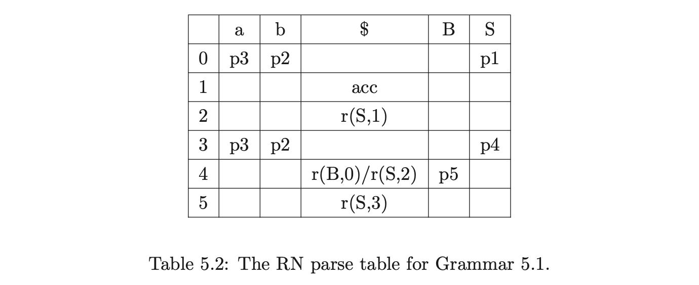
For example, consider the RNGLR parse of the string \(aab\), with Grammar 4.2 and the RN parse table shown in Table 5.2. We begin by creating the state node \(v_{0}\), labelled by the start state \(0\), in \(U_{0}\). Since the only action in \(\mathcal{T}(0,a)\) is a shift to state \(3\), we add \((v_{0},3)\) to \(\mathcal{Q}\) and proceed to execute the Shifter. We create the new node \(v_{1}\), labelled \(3\), in \(U_{1}\) and lookup its associated actions in \(\mathcal{T}(3,a)\). There is only a shift action to state \(3\), so \((v_{1},3)\) is first added to \(\mathcal{Q}^{\prime}\) and then to \(\mathcal{Q}\).
 We continue the parse by shifting the next two input symbols and creating the nodes \(v_{2}\) and \(v_{3}\) in \(U_{2}\) and \(U_{3}\) respectively. Upon the creation of \(v_{3}\) in the Shifterwe encounter a reduction \(r(S,1)\) in \(\mathcal{T}(2,\$)\) and add \((v_{2},S,1)\) to \(\mathcal{R}\).

Processing \((v_{2},S,1)\) in the Reducer we find the shift to state \(4\) in \(\mathcal{T}(3,\$)\). Since there is no node labelled \(4\) in \(U_{3}\) we create \(v_{4}\) and a new edge from \(v_{4}\) to \(v_{2}\). There is a reduce/reduce conflict in \(\mathcal{T}(4,\$)\) so we add \((v_{4},B,0)\) and \((v_{2},S,2)\) to the set \(\mathcal{R}\).

When \((v_{4},B,0)\) is processed by the Reducer the new node \(v_{5}\), labelled \(5\), and the edge from \(v_{5}\) to \(v_{4}\) are created. Although there is a reduction in \(\mathcal{T}(5,\$)\) it is not added to \(\mathcal{R}\). This is a feature of the RNGLR algorithm to prevent reductions that are redundant from being performed. Since the right-nullable reduction \(r(S,2)\) was added to \(\mathcal{T}(4,\$)\) the reduction that would normally be performed after all nullable non-terminals have been reduced was performed early.
We continue the parse by processing \((v_{2},S,2)\), and tracing back a path of length one from \(v_{2}\) to \(v_{1}\). Since there is already node labelled \(4\) in \(U_{3}\) the new edge between \(v_{4}\) and \(v_{1}\) is created. The new edge creates a new reduction path that the reduction \(r(S,2)\) in state \(4\) can be applied down so \((v_{1},S,2)\) is added to \(\mathcal{R}\).
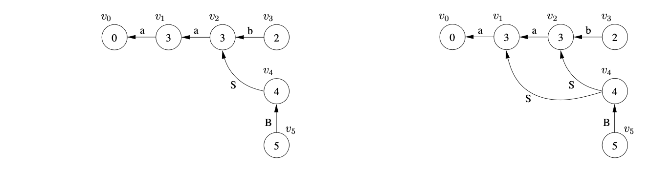
Processing \((v_{1},S,2)\) we trace back a path of length one from \(v_{1}\) to \(v_{0}\) which results in the new state \(v_{6}\) labelled \(1\) and the edge \((v_{6},v_{0})\) being added to the GSS. All of the sets are now empty and since \(U_{3}\) contains a state labelled by the DFA’s accept state, the parse succeeds.

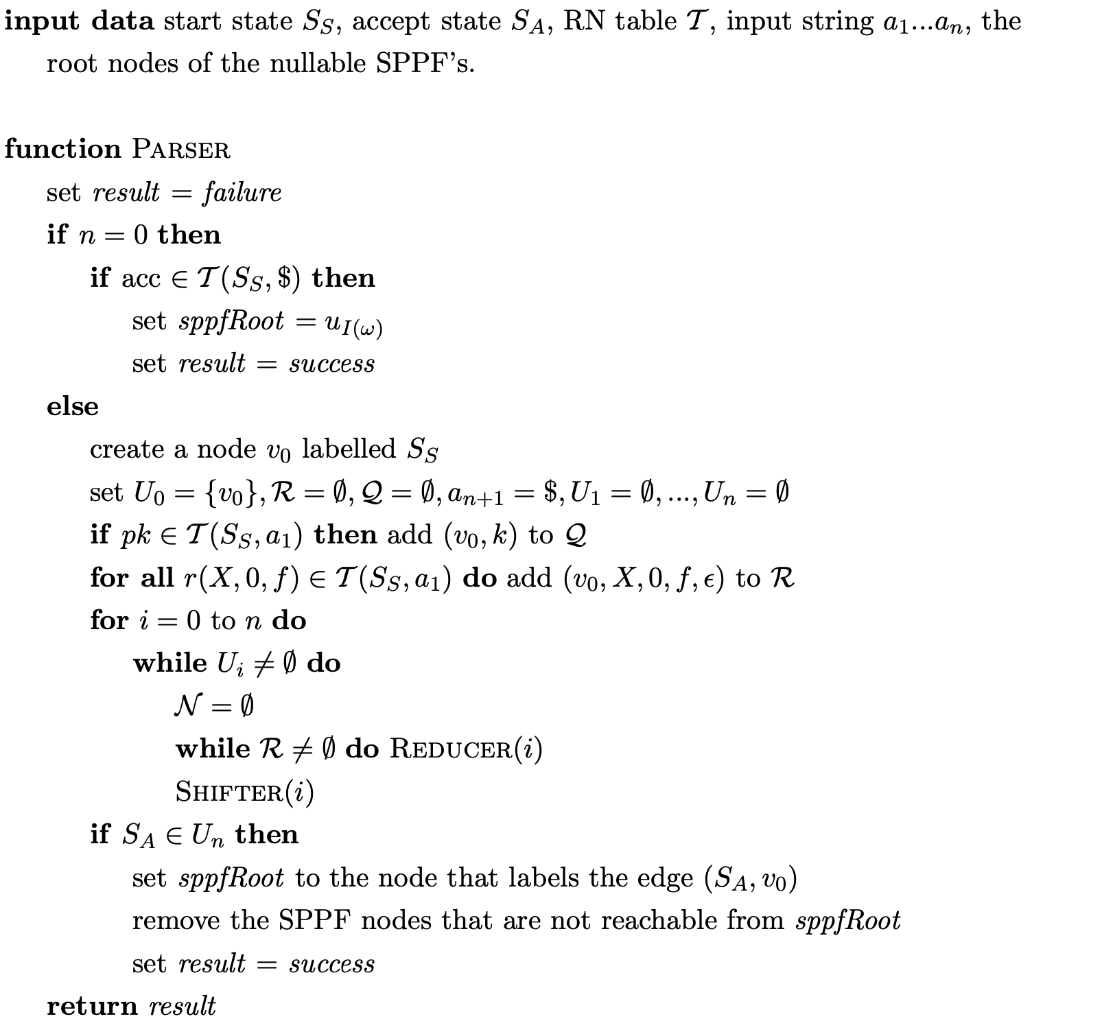
5.5 The RNGLR parsing algorithm
The parser version of the RNGLR algorithm is a straightforward extension of the recogniser described in the previous section. Chapter 4 presented both Tomita’s and Rekers’ approach to the construction of the SPPF. This section provides a brief overview of the main points in that chapter and a discussion of the approach taken by the RNGLR parser.
There are three conflicting goals associated with the construction of an SPPF: building a compact structure; minimising the amount of time taken to build the structure; and ensuring that for ambiguous sentences one derivation tree can be efficiently extracted. Tomita focused on the efficiency of the construction, only implementing a minimal amount of sharing and packing, thereby increasing the space required for the SPPF. Rekers extended Tomita’s approach by increasing the amount of SPPF node sharing at the cost of introducing more searching to the algorithm. The RNGLR parser implements Rekers’ approach in conjunction with several techniques designed to reduce the amount of searching required by the algorithm.
Rekers splits the SPPF nodes into two categories: nodes for the non-terminals called rule nodes and nodes for the terminals called symbol nodes. In order to achieve the sharing in the SPPF the rule and symbol nodes created for the current level are stored in two distinct sets. Before either type of node is created, the required set is searched for an existing node that covers the same part of the input. To do this without having to inspect all the subtrees of a node, the start and end positions of the input that the particular node derives are also stored with the node. A leaf node created for the input symbol at position \(i\), is labelled \((a,i,i)\). A rule node is labelled in a similar way, but takes the first value from its leftmost child and the second value from its rightmost child. So for the input \(a_{1}\ldots a_{d}\), a rule node labelled \((X,j,i)\) means that \(X\stackrel{{*}}{{\Rightarrow}}a_{j}\ldots a_{i}\). If \(X\stackrel{{*}}{{\Rightarrow}}\epsilon\) then \(i,j=0\).
The RNGLR parser implements Rekers’ approach for the construction of the SPPF as opposed to Tomita’s because of the more compact SPPF built. Although both the RNGLR and Rekers’ algorithm build the same SPPF they do so in a slightly different way. Instead of storing the SPPF nodes for the terminals and non-terminals separately, the RNGLR algorithm uses one set called \(\mathcal{N}\) which is reset after each iteration in Parser. In addition to this, because we always know the current level being constructed, only the start position of the string derived is included in an SPPF node. So instead of labeling an SPPF node with a triple \((X,j,i)\), it is labelled with the pair \((X,j)\) and stored in \(\mathcal{N}\).
The RNGLR algorithm only works when used in conjunction with an RN parse table. When a grammar containing right nullable rules is parsed, the right nullable reductions will be done without tracing back over the edges containing the SPPF nodes for the nullable non-terminals. As a result it is necessary to build the SPPF trees forthe nullable non-terminals, and the rightmost nullable strings of non-terminals of a right night nullable rule, before the parse is begun. These nullable trees are called \(\epsilon\)-SPPF trees and since they are constant for a given grammar, they can be constructed when the parser is built and included in the RN parse table. Instead of storing reductions as the tuple \(r(X,m)\), the RN parse table stores the triple \(r(X,m,f)\), where \(X\) is a non-terminal, \(m\) is the length of the reduction and \(f\) is an index into a function \(I\) that returns the root of the associated \(\epsilon\)-SPPF tree. If no \(\epsilon\)-SPPF tree is associated with such a reduction then \(f=0\).
If all the \(\epsilon\)-SPPF trees are created for all the nullable reductions, the final SPPF will not be as compact as it could be. So the \(\epsilon\)-SPPF’s are only constructed for nullable non-terminals and nullable strings \(\gamma\), such that \(|\gamma|>1\) and there is a grammar rule of the form \(A::=\alpha\gamma\), where \(\alpha\neq\epsilon\). Nullable strings like \(\gamma\) are called the required nullable parts. For rules of the form \(A::=\gamma\) where \(\gamma\stackrel{{*}}{{\Rightarrow}}\epsilon\) the \(\epsilon\)-SPPF for \(A\) is used instead.
In order to create the index to the \(\epsilon\)-SPPF trees it is necessary to go through the grammar and, starting at one, index the required nullable parts and the non-terminals that derive \(\epsilon\). Before constructing the \(\epsilon\)-SPPF trees, create the node \(u_{0}\) labelled \(\epsilon\). Then create the \(\epsilon\)-SPPF trees with the root node \(u_{I(\omega)}\), labelled \(\omega\), for the nullable non-terminals or required nullable parts \(\omega\). In the RN parse table for a reduction \((A::=\alpha\cdot\gamma,a)\) write \(r(A,m,f)\), where \(|\alpha|=m\) and \(f=I(\gamma)\) if \(m\neq 0\) and \(f=I(A)\) if \(m=0\).
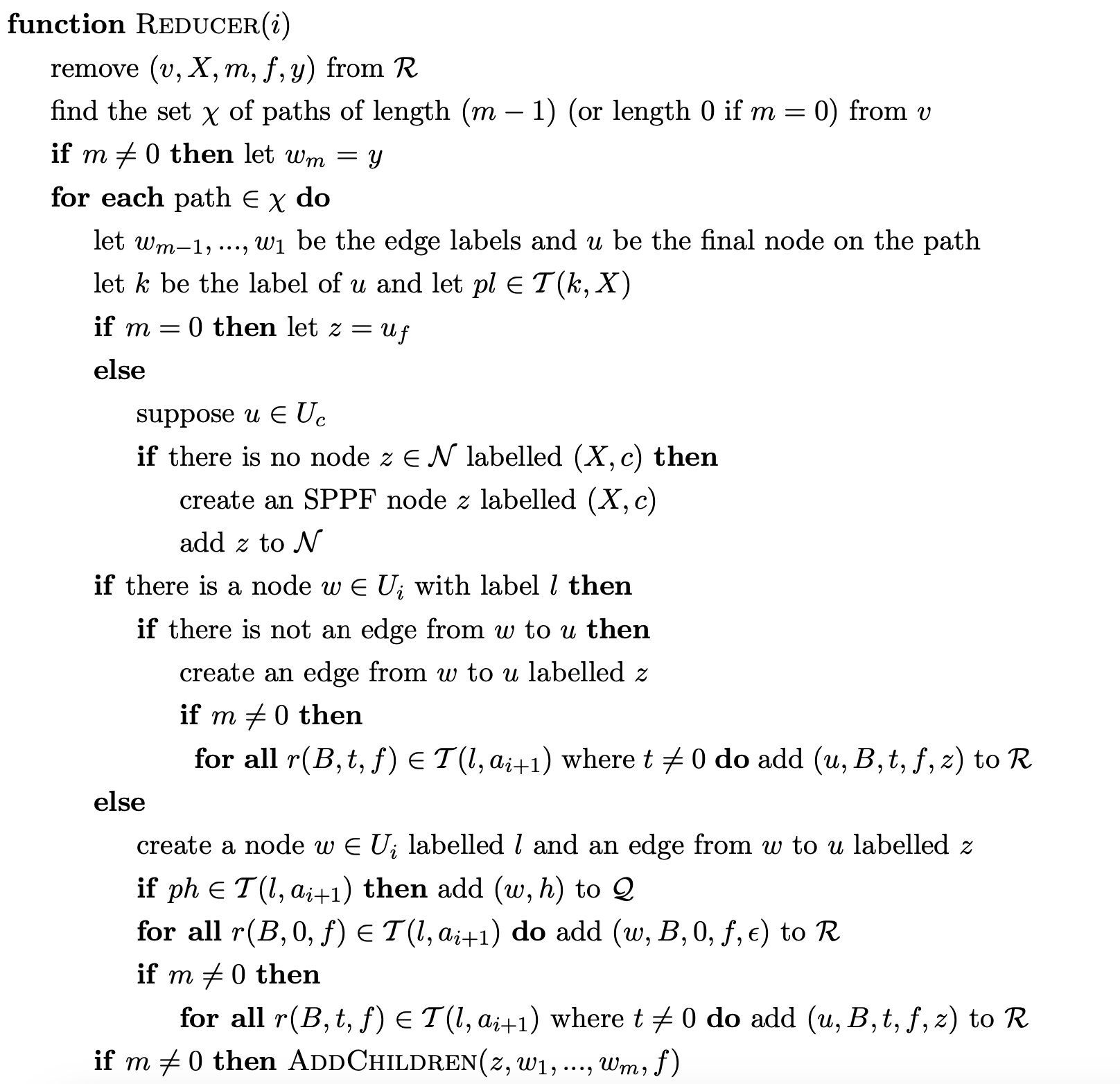
The elements added to the sets \(\mathcal{Q}\) and \(\mathcal{Q}^{\prime}\) are the same as those used by the RNGLR recogniser, but the elements added to \(\mathcal{R}\) contain more information. When a new edge is added between two nodes \(v\) and \(w\), any applicable reductions from \(v\) are added to the set \(\mathcal{R}\). For a reduction of the form \(r(X,m,f)\), where \(m>0\), we add \((w,X,m,f,z)\) to the set \(\mathcal{R}\). The first three elements, \(w,X,m\) are the same as those used in the recogniser (state node, non-terminal, length of reduction). If the reduction is an RN-reduction of the form \((X::=\alpha\cdot\beta)\) then \(f\) is the index into the function \(I\) which stores the root node of the \(\epsilon\)-SPPF for \(\beta\) and \(z\) is the SPPF node that labels the edge between \(v\) and \(w\). If the length of the reduction is zero (\(m=0\)) then \(f\) is the index into \(I\) for the root of the \(\epsilon\)-SPPF of \(X\) and \(z\) is \(\epsilon\), since the edge between \(v\) and \(w\) is not traversed.
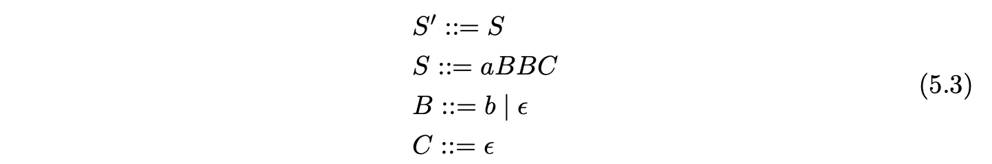
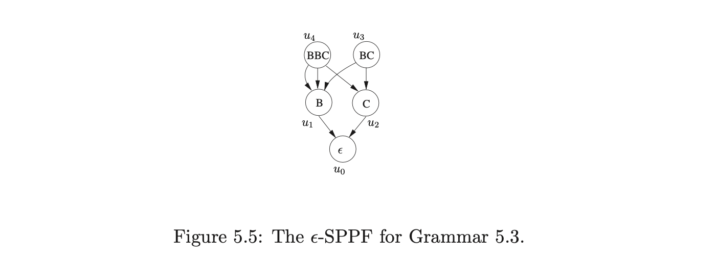
For example, consider Grammar 5.3. The nullable non-terminals are \(B\) and \(C\), and the required nullable parts are \(BBC\) and \(BC\). We define \(I(B)=1\), \(I(C)=2\), \(I(BC)=3\) and \(I(BBC)=4\). The associated \(\epsilon\)-SPPF is shown in Figure 5.5.
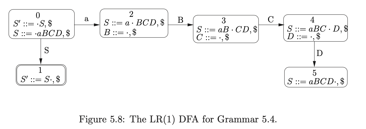
 Before presenting the formal specification of the RNGLR parser we demonstrate how the GSS and SPPF are constructed for the parse of the string \(ab\) in Grammar 5.3. The associated LR(1) DFA and RN parse table are shown in Figure 5.6 and Table 5.4.
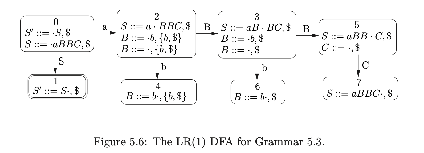
 We create \(v_{0}\), labelled by the start state of the DFA, and add it to \(U_{0}\). Since the only applicable action in \(\mathcal{T}(0,a)\) is a shift to state 2, we add \((v_{0},2)\) to \(\mathcal{Q}\). The Shifter removes \((v_{0},2)\) from \(\mathcal{Q}\) and creates a new SPPF node, \(w_{1}\), labelled \((a,1)\). Then since no node labelled 2 exists in the next level, \(v_{1}\) is created and added to \(U_{1}\), with an edge back to \(v_{0}\) labelled by \(a\) and \(w_{1}\). There is a shift/reduce conflict in \(\mathcal{T}(2,b)\): a shift to state \(4\) and a reduction \(r(B,0,1)\). We add \((v_{1},4)\) to \(\mathcal{Q}^{\prime}\) and \((v_{1},B,0,1,\epsilon)\) to \(\mathcal{R}\).
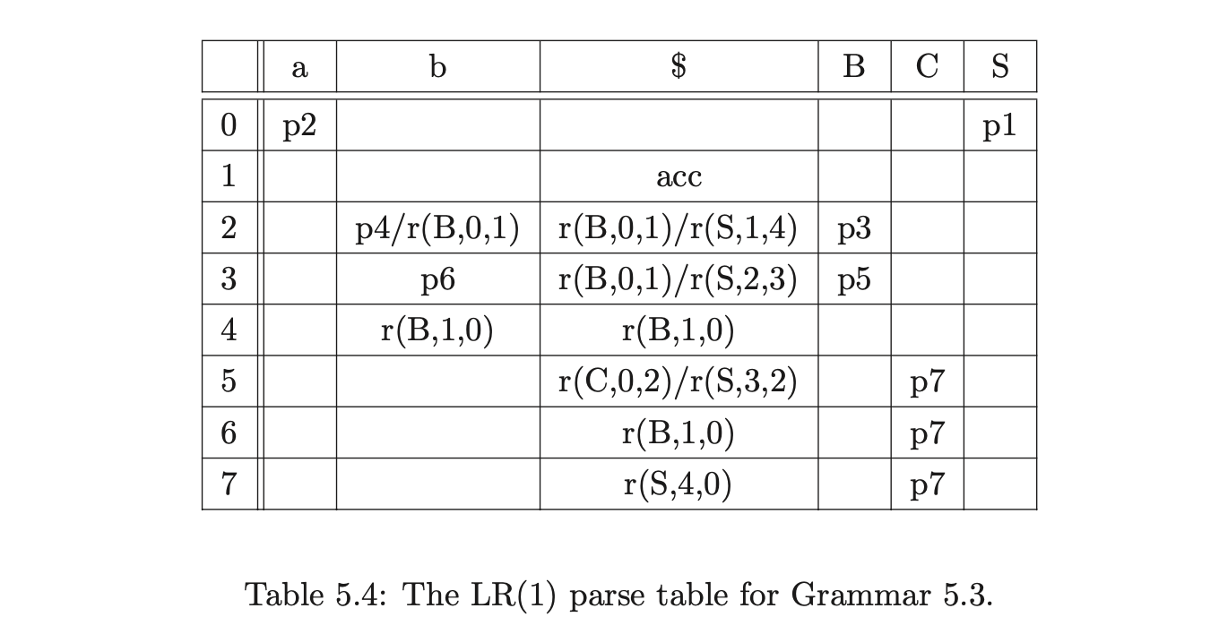
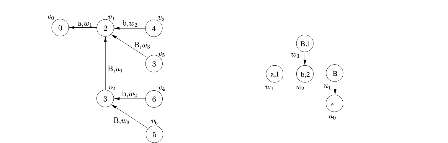
This completes the construction of the first level and the initialisation of \(U_{1}\). The GSS and SPPF constructed up to this point are shown below.
 Next we process the reduction \((v_{1},B,0,1,\epsilon)\) in the Reducer. It is a nullable reduction so we do not trace back a path in the GSS, but we do create the new node, \(v_{2}\), labelled \(3\), with an edge back to \(v_{1}\). We label the edge by the non-terminal of the reduction, \(B\), and the root of the \(\epsilon\)-SPPF tree for \(B\). Since there is a shift action in \(\mathcal{T}(3,b)\) we add \((v_{2},6)\) to \(\mathcal{Q}\).
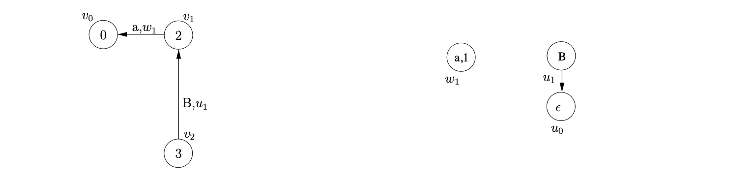
Processing the two queued shift actions in \(\mathcal{Q}\) results in the construction of the SPPF node \(w_{2}\) and the two new GSS nodes \(v_{3}\) and \(v_{4}\). There is a reduction \(r(B,1,0)\) from both nodes, so we add \((v_{1},B,1,0,w_{2})\) and \((v_{2},B,1,0,w_{2})\) to \(\mathcal{R}\).
Processing the first of these reductions, we create the new SPPF node, \(w_{3}\), labelled \((B,1)\), add it to the set \(\mathcal{N}\) and then use it to label the edge between the new GSS node, \(v_{5}\), and \(v_{1}\). We make the SPPF node, \(w_{2}\), that labelled the edge between \(v_{3}\) and \(v_{1}\) the child of \(w_{3}\). Since there is a reduce/reduce conflict, \(r(B,0,1)\) and \(r(S,2,3)\), in \(\mathcal{T}(3,\$)\) we add \((v_{5},B,0,1,\epsilon)\) and \((v_{1},S,2,3,w_{3})\) to \(\mathcal{R}\). When we process the queued reduction \((v_{2},B,1,0,w_{2})\) we create the new GSS node \(v_{6}\) labelled \(5\) and an edge to \(v_{2}\). However, because there has already been the SPPF node, \(w_{3}\), labelled \((B,1)\) created in the current step of the algorithm (and stored in the set \(\mathcal{N}\)) we re-use it to label the edge between \(v_{6}\) and \(v_{2}\).
At this point \(\mathcal{R}=\{(v_{5},B,0,1,\epsilon),(v_{1},S,2,3,w_{3}),(v_{6},C,0,2,\epsilon),(v_ {2},S,3,2,w_{3})\}\). We remove and process the first of these reductions which results in the new edge, labelled \((B,u_{1})\), being added between \(v_{6}\) and \(v_{5}\). Although the new edge has introduced a new reduction path from \(v_{6}\), we do not add anything to the set \(\mathcal{R}\) because the reduction performed was of length zero.
Next we process \((v_{1},S,2,3,w_{3})\). We trace back a path of length one from \(v_{1}\) to \(v_{0}\), collecting the SPPF node, \(w_{1}\), that labels the edge traversed. We create the new GSS node, \(v_{7}\), labelled \(1\) and an edge between \(v_{7}\) and \(v_{0}\). We create the new SPPF node, \(w_{4}\), labelled \((S,0)\) with edges pointing to the nodes \(w_{1},w_{3}\) and \(u_{3}\) and use it to label the edge between \(v_{7}\) and \(v_{0}\) in the GSS. We also add \(w_{4}\) into the set \(\mathcal{N}\).
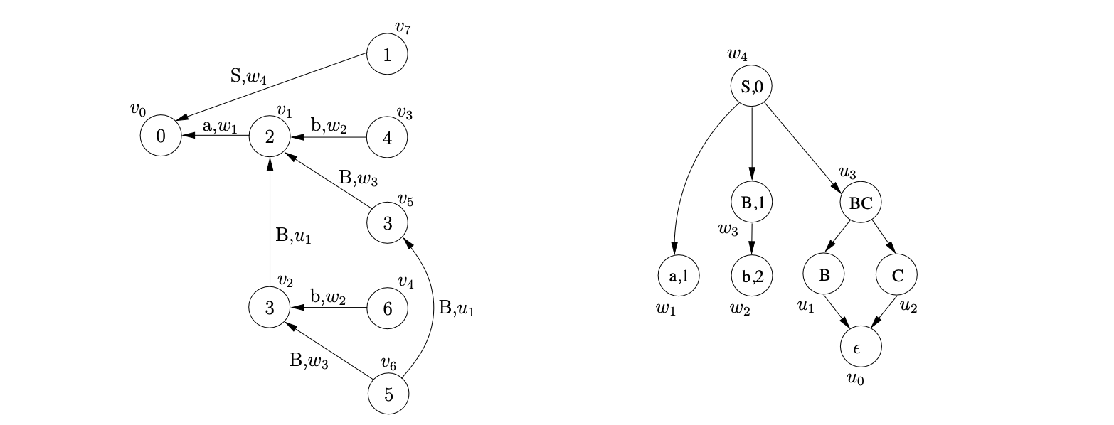
Processing the reduction encoded by \((v_{6},C,0,2,\epsilon)\) we create the new GSS node \(v_{8}\), labelled \(7\), and an edge from \(v_{8}\) to \(v_{6}\). Since the reduction is nullable, we label the new edge by the \(\epsilon\)-SPPF node \(u_{2}\) and do not add any other reductions to \(\mathcal{R}\).
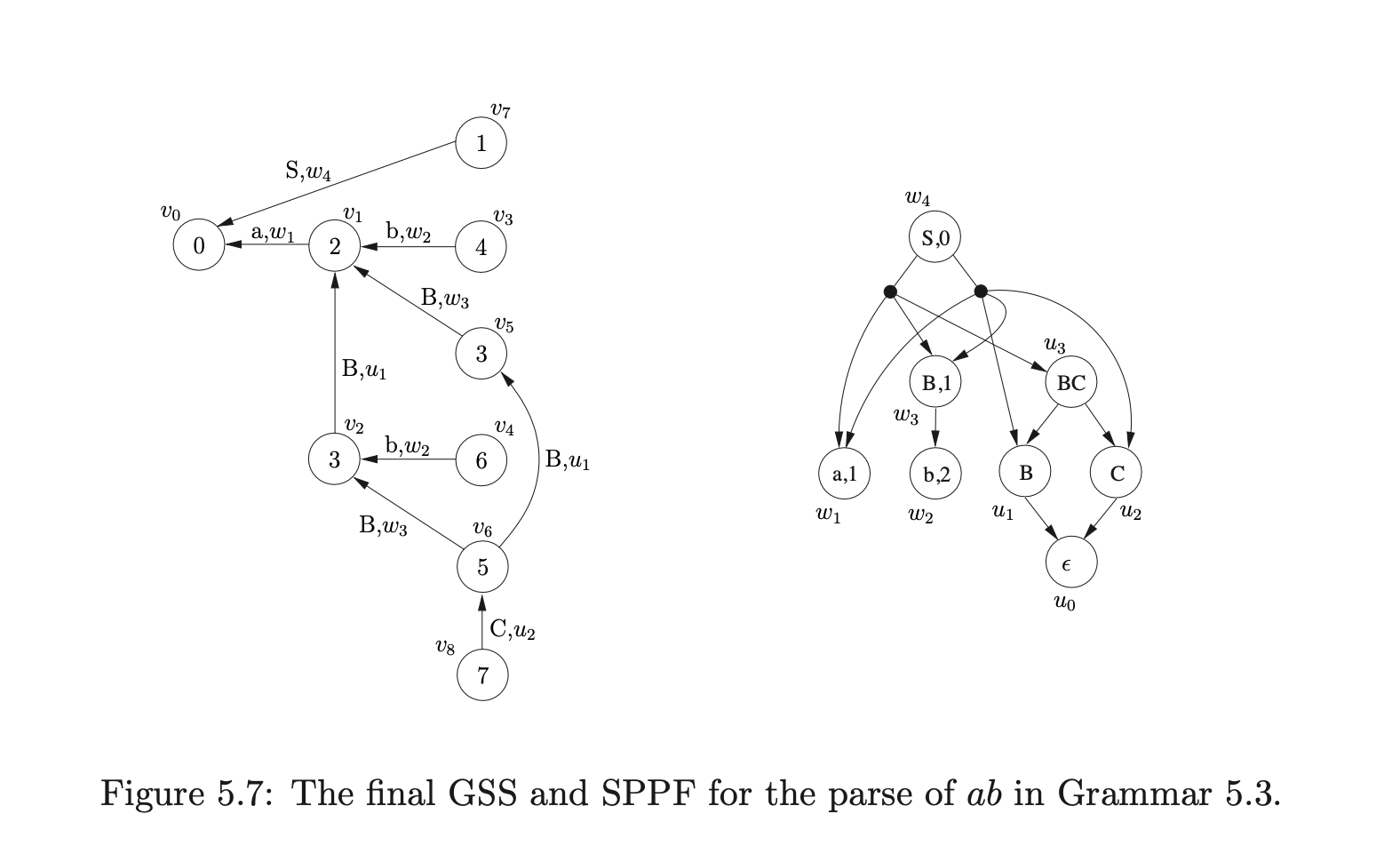
We then process the final reduction in \(\mathcal{R}\), \((v_{2},S,3,2,w_{3})\). We trace back a path of length two from \(v_{2}\) to \(v_{0}\) and collect the SPPF nodes \(u_{1}\) and \(w_{1}\) that label the traversed edges. We search the set \(\mathcal{N}\) for a node labelled \((S,0)\) and find \(w_{4}\). Since it does not have a sequence of children \([w_{1},u_{1},w_{3},u_{2}]\) we create two new packing nodes below \(w_{4}\) and add the existing children of \(w_{4}\) to one and the new sequence to the other.
At this point all the input string has been parsed and no other actions remain to be processed. Since the accept state of the DFA labels \(v_{7}\), the parse is successful and the root of the SPPF is the node that labels the edge between \(v_{7}\) and \(v_{0}\), \(w_{4}\). The final GSS and SPPF constructed during the parse are shown in Figure 5.7.
RNGLR parser
5.6 Resolvability
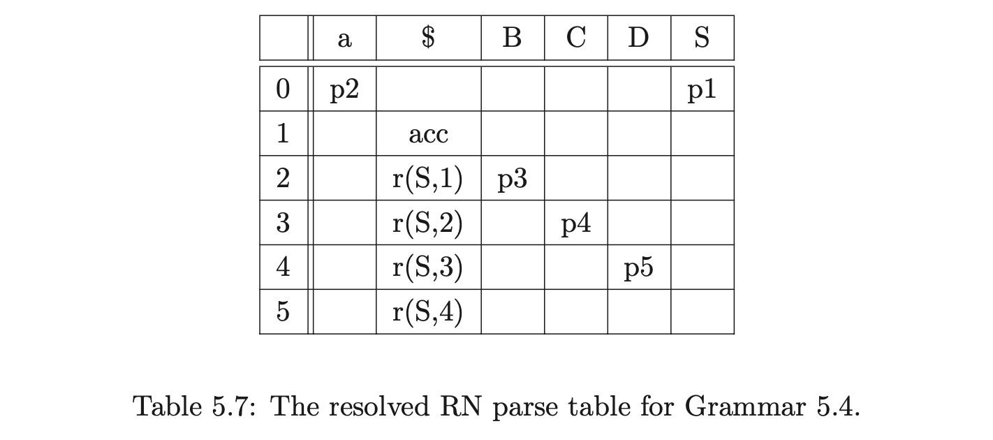
In Section 5.3 we discussed the effect of the extra non-determinism created as a result of the nullable reductions added to the RN parse table. In this section we present an approach, first described in [10], of removing redundant nullable reductions from the RN parse table of LR grammars with right nullable rules. In certain cases this new resolved parse table can be used by the standard LR parsing algorithm, to parse certain strings with less stack activity. It has been shown in [10] that for an LR grammar it is possible to remove all reduce/reduce conflicts from an RN parse table so that the standard LR parsing algorithm can be used to parse sentences with less stack activity.
In order to remove reductions from a state \(k\) without breaking the parser, it is necessary for \(k\) and a lookahead \(a\) to conform to the following two properties.
For each \(a\in\mathbf{T}\cup\{\$\}\) there is at most one item \((X::=\tau\cdot\sigma,a)\in k\), such that \(\tau\neq\epsilon\) and \(\sigma\stackrel{{*}}{{\Rightarrow}}\epsilon\).
If \((X::=\tau\cdot\sigma,a)\in k\), where \(\sigma\stackrel{{*}}{{\Rightarrow}}\epsilon\), and \((W::=\alpha\cdot\beta,g)\in k\), where \(a\in\text{FIRST}(\beta)\), then \(\tau=\epsilon\) and any derivation \(\beta\stackrel{{*}}{{\Rightarrow}}au\) includes a step \(Xau\stackrel{{*}}{{\Rightarrow}}\sigma au\).
Such states are called a-resolvable. The two properties above work on the principle that a state \(k\) with an item of the form \((X::=\tau\cdot\sigma,a)\), where \(\tau\neq\epsilon\) and \(\sigma\stackrel{{*}}{{\Rightarrow}}\epsilon\) can have all but one of its reductions, for the lookahead \(a\), removed as long as property 2 is not broken. This is because we can define the order in which rules are added toa DFA state and hence guarantee that the reduction for the rule \(X::=\tau\sigma\) must take place before any other action can happen.
The reduction that is not removed from an a-resolvable state \(k\) is known as the base reduction of \(k\) for lookahead \(a\). To formally define a base reduction it is necessary to first define a function to calculate the order in which items are added to a DFA state.
Definition 5.1: Let \(k\) be a DFA state and let \((X::=\tau\cdot\sigma,a)\) be an item in \(k\). If \(\tau=\epsilon\) then we define \(level_{k}(X::=\tau\cdot\sigma,a)=0\). We also define \(level_{0}(S^{\prime}::=\cdot S,\$)=0\). For \(X\neq S^{\prime}\) and \(\tau=\epsilon\) we let

and then define \(level_{k}(X::=\cdot\sigma,a)=(r+1)\). [SJ03a]
Definition 5.2: Let \(\Gamma\) be any context-free grammar and let \(k\) be an \(a\)-resolvable state in the DFA for \(\Gamma\). An item \((X::=\tau\cdot\sigma,a)\in k\) is a base reduction on \(a\) in \(k\) if, for all other items \((Y::=\gamma\cdot\delta,a)\in k\) such that \(\delta\stackrel{{*}}{{\Rightarrow}}\epsilon,level_{k}(X::=\tau \cdot\sigma,a)\leq level_{k}(Y::=\gamma\cdot\delta,a)\).[10]
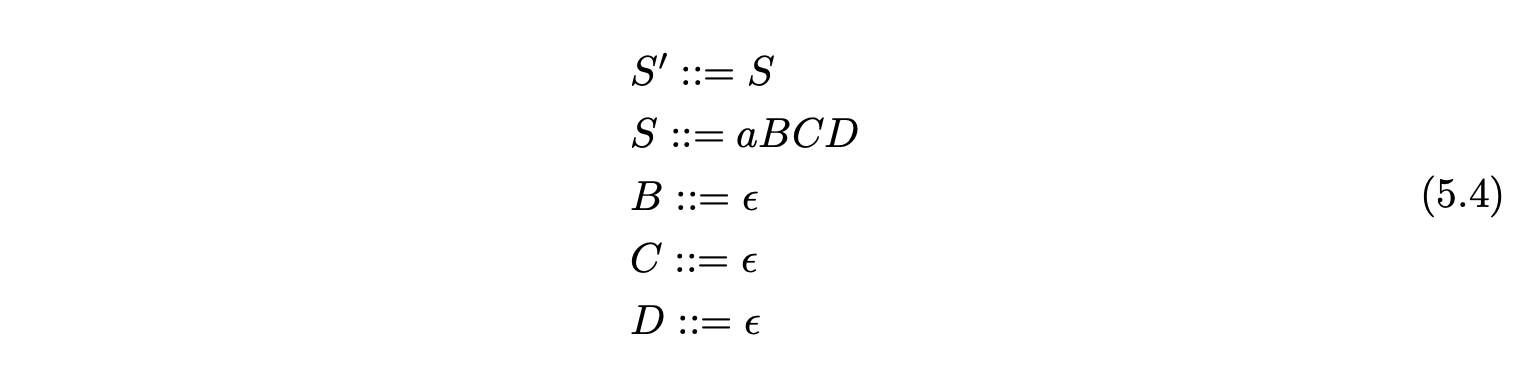
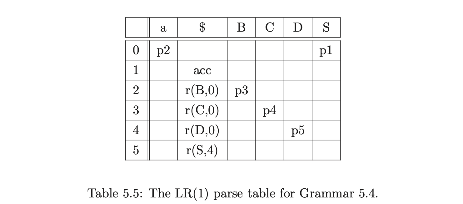
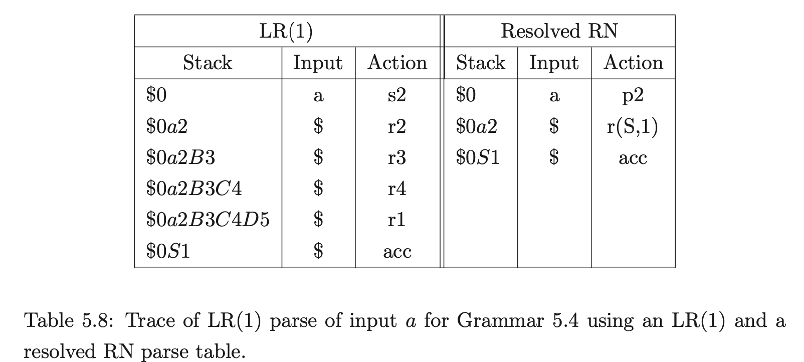
Table 5.8 shows how the resolved RN parse table of the LR(1) grammar 5.4 can be used by the standard LR(1) parsing algorithm, to parse a sentence using less stack activity than when the LR(1) table is used.
5.7 Summary
This chapter has presented Algorithm 1e - a straightforward extension of Tomita’s Algorithm 1 that can deal with hidden-left recursion, but which fails to parse grammars containing hidden-right recursion. A modification to the standard LR(1) parse table was introduced which causes Algorithm 1e to correctly parse all context-free grammars. Tables containing this modification are called RN tables. The RNGLR recognition algorithm that parses all context-free grammars with the use of an RN parse table was described and its operation demonstrated with various examples. The RNGLR parser that constructs an SPPF in the style of Rekers, but which employs less searching, was also presented.
Chapter 10 presents the experimental results that abstract the performance of Algorithm 1e, Algorithm 1e mod, and the RNGLR algorithm for grammars which trigger worst case behaviour and several programming language grammars and strings.