7.Reduction Incorporated Generalised LR parsing
The most efficient general parsing algorithm to date achieves \(O(n^{2.376})\) worst case time complexity. Unfortunately, as already discussed in the previous chapter, the high constants of proportionality associated with this technique make it impractical for all but the longest strings.
This thesis focuses on the general parsing algorithms based on Tomita’s GLR parsing technique. The initial goal of GLR parsing was to provide an efficient algorithm for “practical natural language grammars” [126] by exploiting the efficiency of Knuth’s deterministic LR parser. The BRNGLR algorithm, presented in Chapter 6, is a GLR parsing algorithm that achieves \(O(n^{3})\) worst case complexity. Although the worst case is not always reached, the run time of the algorithm is far from ideal, especially when compared to the deterministic techniques.
Since the run time of a parser is highly visible to a user, there have been several attempts at speeding the run time of LR parsers [1, 2, 126, 127]. Most of these have focused on achieving speed ups by implementing the handle finding automaton in low-level code. A different approach to improving efficiency is presented in [1, 2], the basic ethos of which is to reduce the reliance on the stack. It is clear that the run time performance of shift-reduce parsers is dominated by the maintenance of the parse stack. The recognition of regular languages that are defined by regular expressions, is much more efficient than the parsing of context-free languages that are defined by context-free grammars because only the current state needs to be stored. Informally, Aycock and Horspool’s idea uses FA based recognition techniques for the regular parts of a grammar and only uses a stack for the parts of the grammar which are not regular. (We shall define this formally in detail below.)
Unfortunately, as the authors point out, the algorithm presented in [1] fails to terminate on grammars that contain hidden-left recursion. This chapter presents the Reduction Incorporated Generalised LR (RIGLR) algorithm that is based on thesame approach taken by Aycock and Horspool, but which can be used to parse all context-free grammars correctly. As part of the work in this thesis, the RIGLR algorithm was implemented for comparison with the RNGLR and BRNGLR algorithms. The theoretical description of the RIGLR algorithm given here is taken primarily from [15].
We begin by discussing the role of the stack in a shift-reduce parser and then show how to split a grammar, \(\Gamma\), into several new grammars for some of the non-terminals that define a regular part of \(\Gamma\). We then describe the construction of the Intermediate Reduction Incorporated Automata (IRIA) that accept the strings in the language of these regular parts and then use the subset construction algorithm to construct the more deterministic Reduction Incorporated Automata (RIA). Combining the separate RIA to produce the Recursion Call Automaton (RCA) we can recognise the strings in the language of \(\Gamma\) with less stack activity than the GLR parsing techniques. We then introduce the RIGLR algorithm that uses a similar structure to Tomita’s GSS to parse all context-free grammars. The chapter concludes with a discussion on the construction of derivation trees for this algorithm.
7.1 The role of the stack in bottom-up parsers
The DFA’s associated with the deterministic bottom-up shift-reduce parsers act as handle recognisers for parsing algorithms. A parse is carried out by reading the input string one symbol at a time and performing a traversal through the DFA from its start state. If an accept state is reached from the input consumed, then the leftmost handle of the input has been located. At this point the parser replaces the string of symbols in the input that match the right hand side of the handle’s production rule, with the non-terminal on the left hand side of the production rule. Parsing then resumes with the modified input string from the start state of the DFA. If an accept state is reached and the start symbol is the only symbol in the input string, then the original string is accepted by the parser.
The approach of repeatedly feeding the input string into the DFA is clearly inefficient. The initial portion of the input may be read several times before its handle is found. Consequently a stack is used to push symbols on when they are read and pop them off when a handle is found. This prevents the initial portion of the input being repeatedly read.
Many parser generators employ an extended BNF notation (EBNF), which includes regular expression operators to encourage structures to be defined in a way that can be efficiently implemented. Although the stack improves a parser’s run time, there are overheads associated with its use, so it is not uncommon for language developers to try and optimise its use; left recursion is preferred to right recursion in bottom-up parsers as the latter causes a deep stack to be created whereas the former yields a shallow stack.
For example, consider the two grammars defined below. Both accept all strings of \(a\)s, but the one on the left uses left recursion whereas the one on the right uses right recursion.
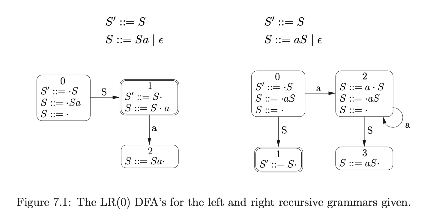
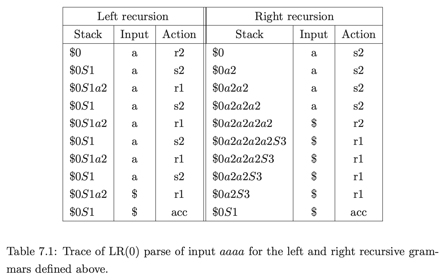
A trace of the stacks used during a parse of the string \(aaaa\), for both grammars defined above, is shown in Table 7.1. The parse of the right recursive grammar shows that the parser needs to remember the entire left context so it can reduce \(a\) the correct number of times. This results in a deeper stack being created.
Since a grammar’s DFA is deterministic, one might expect that a path can simply be re-traced once a handle is found without the use of a stack. If this was the case then we could add an \(\epsilon\)-edge from each state with a reduction \((X::=\alpha\cdot)\) to the state at the end of the reduction path whose target is \(X\). For example, consider Grammar 7.1 and the NFA shown in Figure 7.2. We have added reduction transitions, labelled \(\mathcal{R}i\) where \(i\) is the rule number of the production used in the reduction, to the DFA states that contain items of the form \((X::=\alpha\cdot)\).
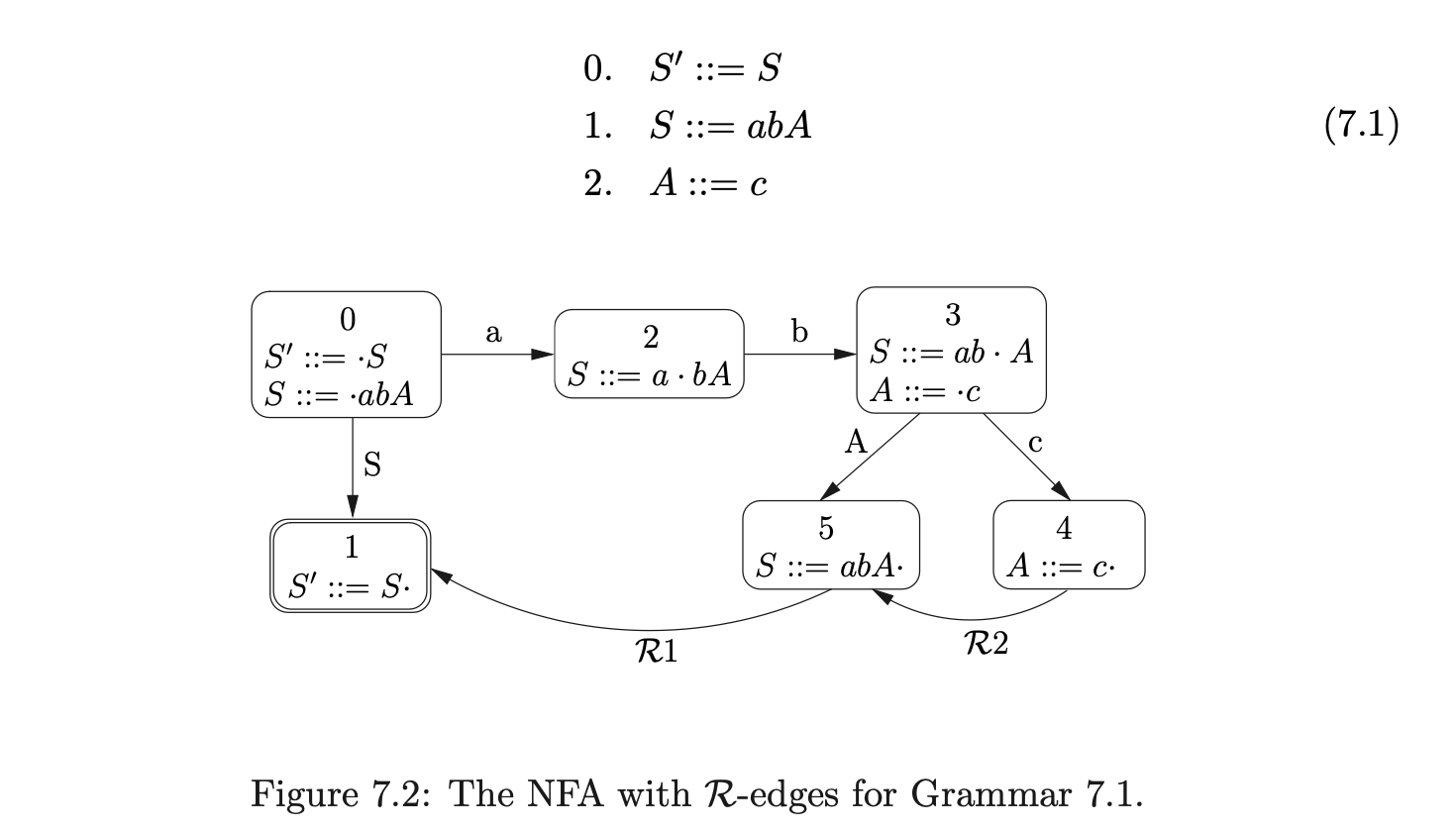
Recall from the Chomsky hierarchy in Chapter 2 that the FA can be used to recognise languages defined by regular grammars. Although Grammar 7.1 is context-free, it defines a regular language. It is therefore not a big surprise that it can be parsed without the use of a stack. Unfortunately, the problem of deciding whether the language of a context-free grammar is regular or not is known to be undecidable [1] and anyway, certain grammars that satisfy this property are difficult to parse without a stack. For example, consider Grammar 7.2 that defines the regular language \(\{bad,dac\}\) and the NFA shown in Figure 7.3.
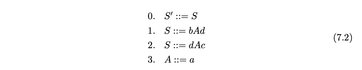
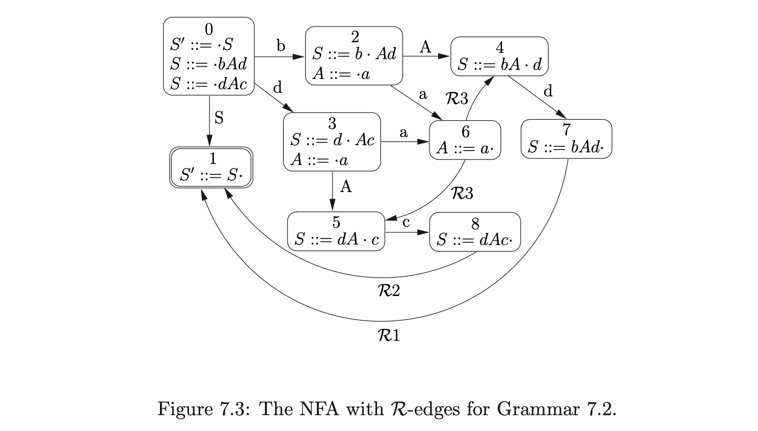
Using the NFA above it is possible to reach state 6 after consuming \(ba\) or \(da\). The state that we should move to after performing the reduction in state 6 depends upon the path that we have taken to get there. After shifting \(ba\) we should move to state 4, but after shifting \(da\) we should move to state 5. However, because there are two \(\mathcal{R}\)-edges leaving state 6 we do not know which one to follow. Using the NFA in Figure 7.3 it is possible to accept the strings \(bad\) and \(dac\) which are not in the language of Grammar 7.2. This is caused by certain multiple instances of non-terminals occurring on the right hand side of production rules. In the example above, it is the non-terminal \(A\) that causes the problem. In a standard LR parser, the stack ensures that the correct path is re-traced in such instances preventing incorrect strings being accepted.
Although one may expect that it is possible to recognise some grammars with multiple instances of non-terminals, since they can be regular and by definition accepted by the FA alone, there are some grammars that contain inherently context-free structures. For example, self embedded recursion is a context-free structure that cannot be recognised by a FA alone. Consider Grammar 7.3 and the NFA constructed with the \(\mathcal{R}\)-edges shown in Figure 7.4.
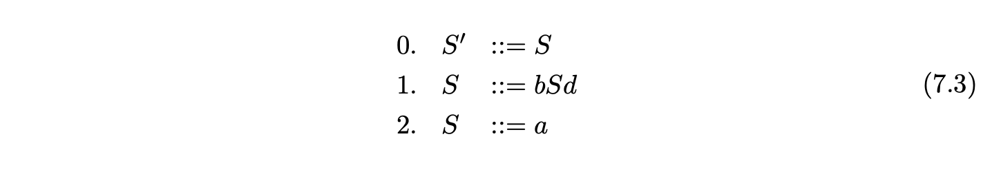
Grammar 7.3 defines the language which contains strings of the form \(b^{k}ad^{k}\) for any \(k\geq 0\). In other words it accepts strings with an equal, or balanced, number of \(b\)s and \(d\)s. Although the NFA in Figure 7.4 correctly recognises these strings, it also accepts strings of the form \(b^{i}ad^{j}\) where \(i\geq 0\) and \(j\geq 0\), which are not in the language defined by the grammar.
The problem with using an NFA without a stack to recognise a context-free language is caused by the NFA not being able to’remember’ what it has already seen. A stack can be used to ensure that once \(k\)bs have been shifted, the parser will reduce exactly \(k\) times.
7.2 Constructing the Intermediate Reduction Incorporated Automata
We have seen in the previous section that a stack is an important part of any shift-reduce parser. A stack guarantees that:
when there are multiple instances of non-terminals on the right hand side of the production rules, the parser will move to the correct state after performing a reduction;
when an instance of self embedded recursion, \(A\stackrel{{+}}{{\Rightarrow}}\alpha A\beta\), is encountered during a parse the number of matches to \(\alpha\) equals the number of matches to \(\beta\).
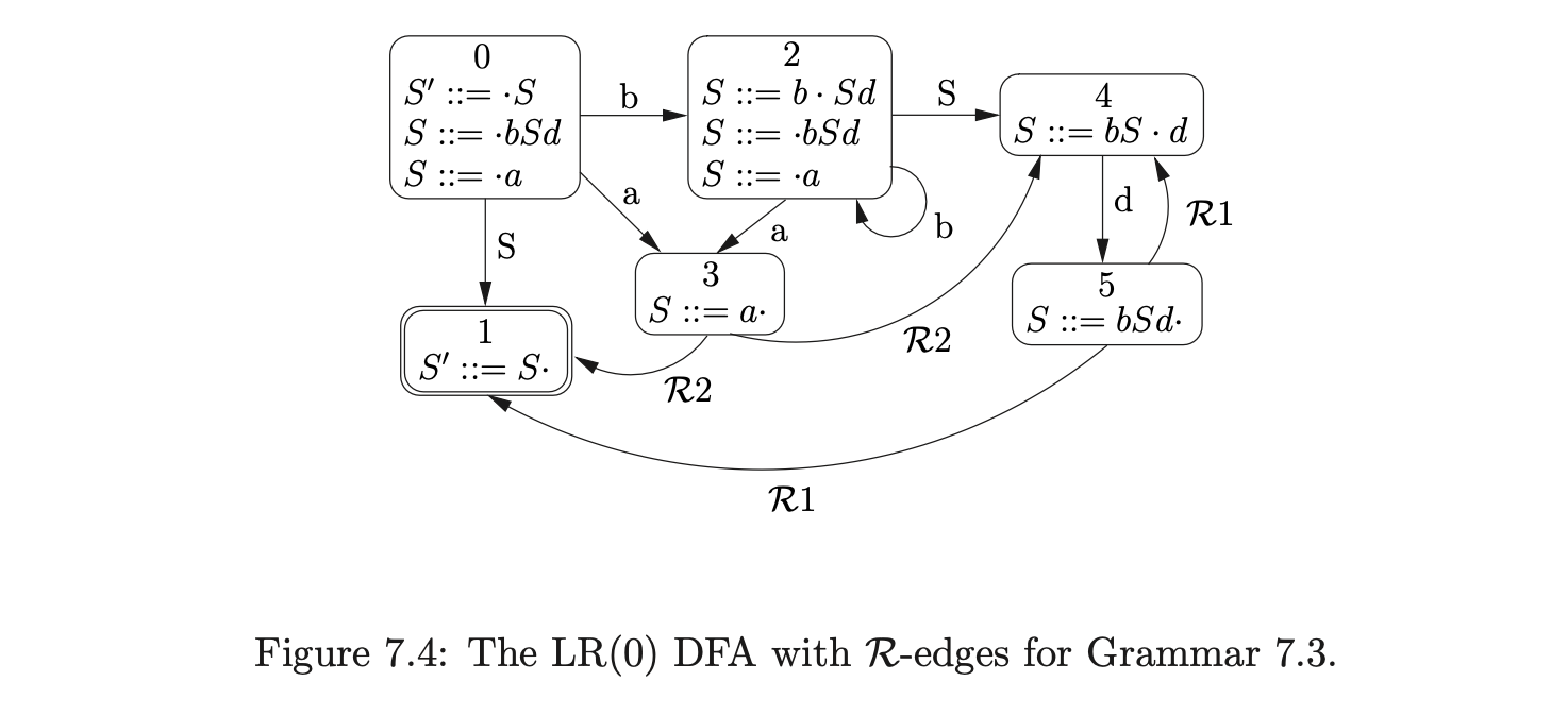
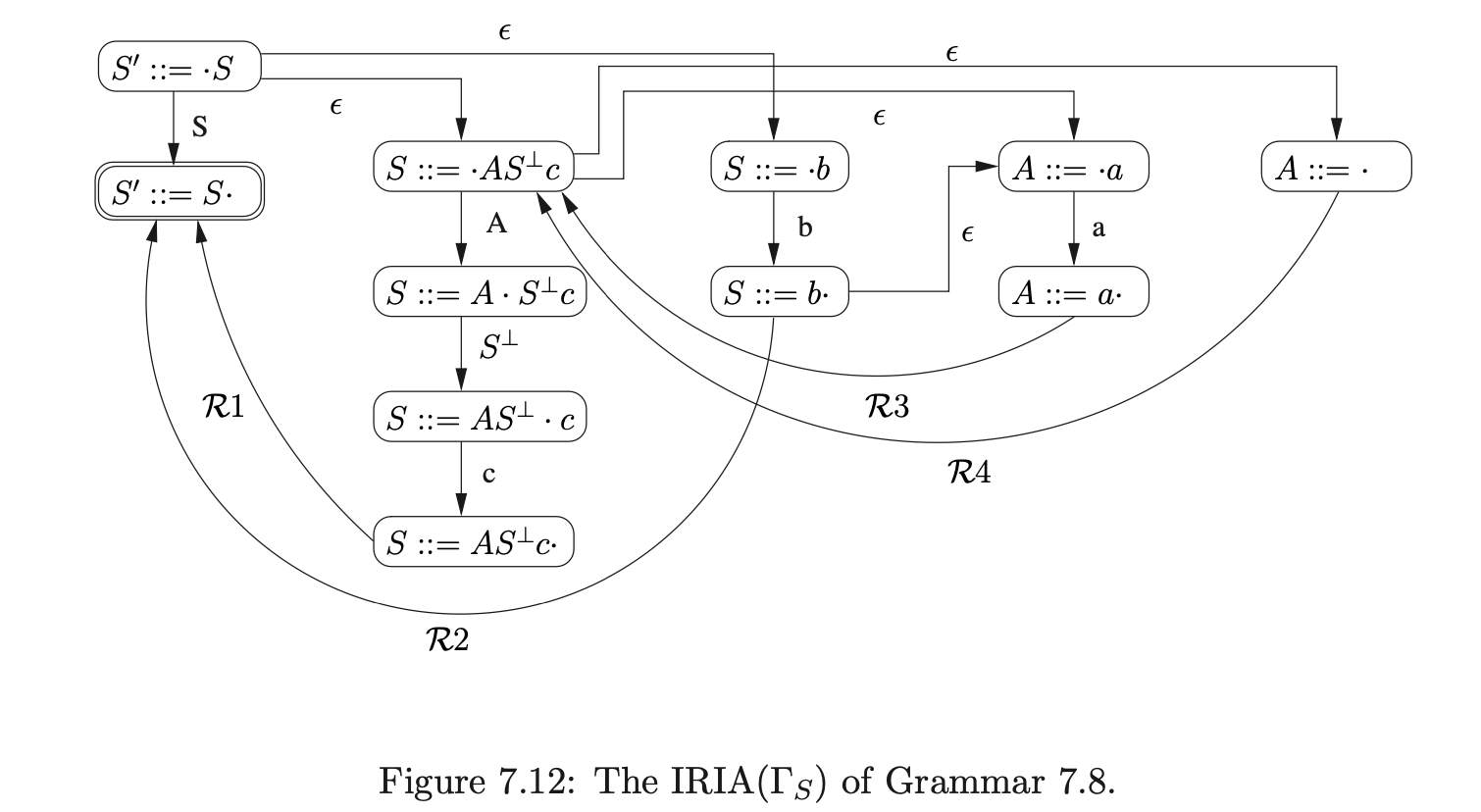
Although a stack is necessary to correctly recognise the portions of a derivation that rely on the self embedded non-terminals, we can deal with the multiple instances of non-terminals by’multiplying out’ some of the states in the FA. Recall, from Chapter 2, that we construct the LR(0) NFA of a grammar by first creating the individual automata for each of the production rules and then join them together with \(\epsilon\)-edges when a state contains an item with a dot before a non-terminal. For each occurrence of a non-terminal that is encountered in an item, we create a new NFA for that non-terminal’s production rule. We now extend this approach by adding extra NFA states for multiple instances of non-terminals. For example, consider Grammar 2.7, on page 31, and the NFA that has been’multiplied out’ in Figure 7.5.
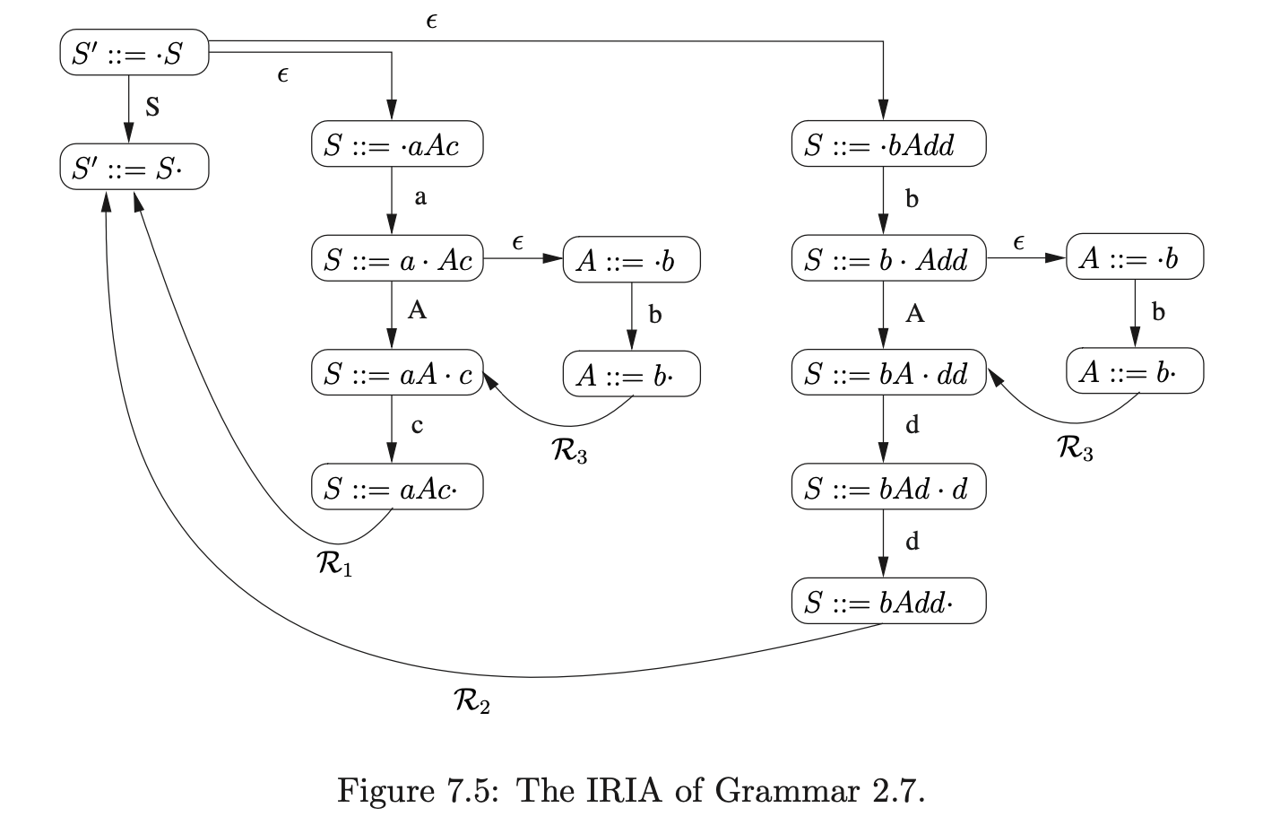
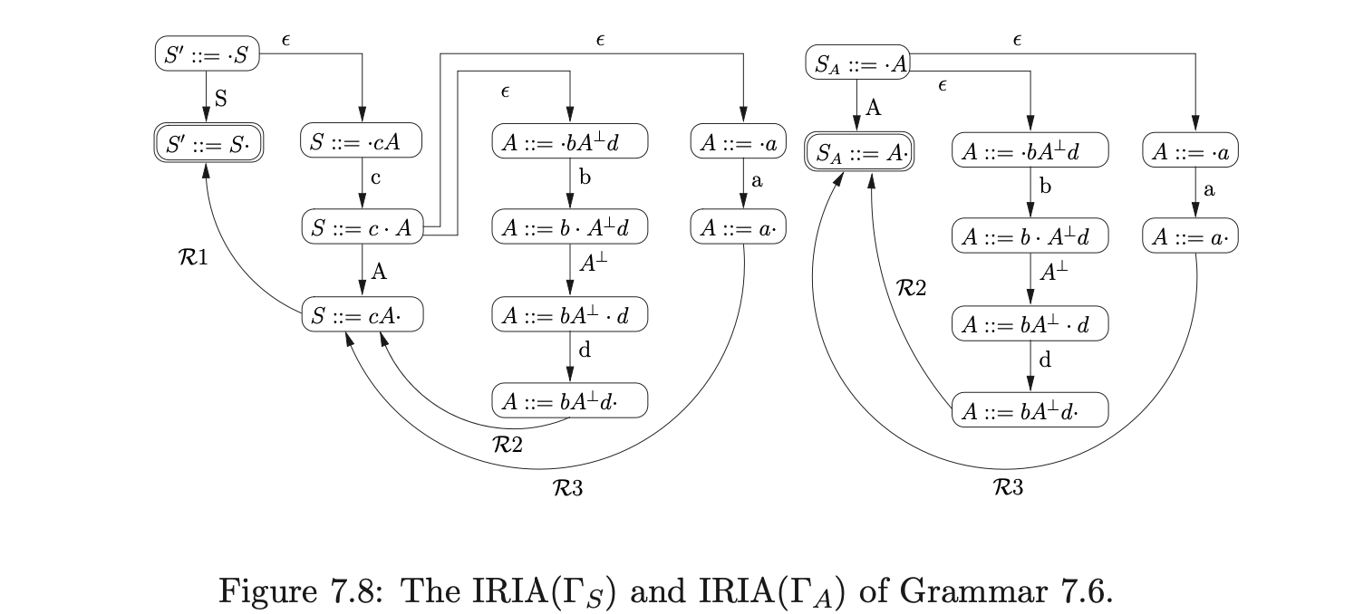
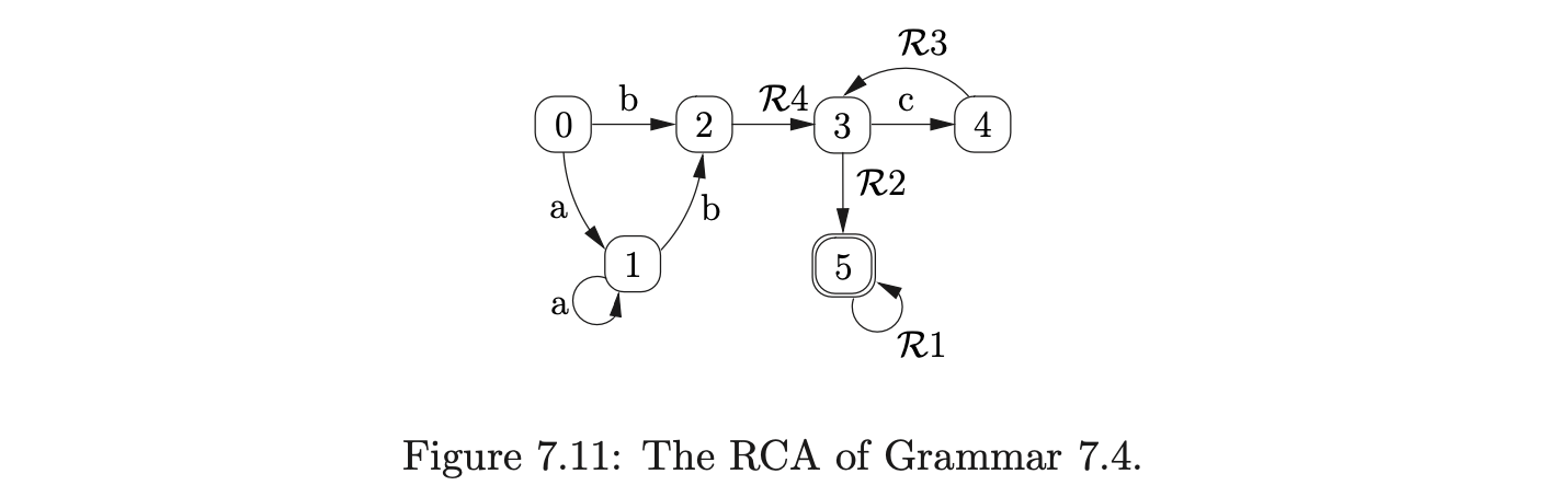
However, if we multiplied out all instances of non-terminals in this way, any recursive rules would result in an infinite number of states being created. For this reason, a recursive instance of a non-terminal \(B\), in a state that contains an item of the form \((A::=\alpha\cdot B\beta)\), has an \(\epsilon\)-edge back to the most recent state, on a path from the start state to the current state, that contains an item of the form \((B::=\cdot\gamma)\). For example consider Grammar 7.4 and the IRIA shown in Figure 7.6.
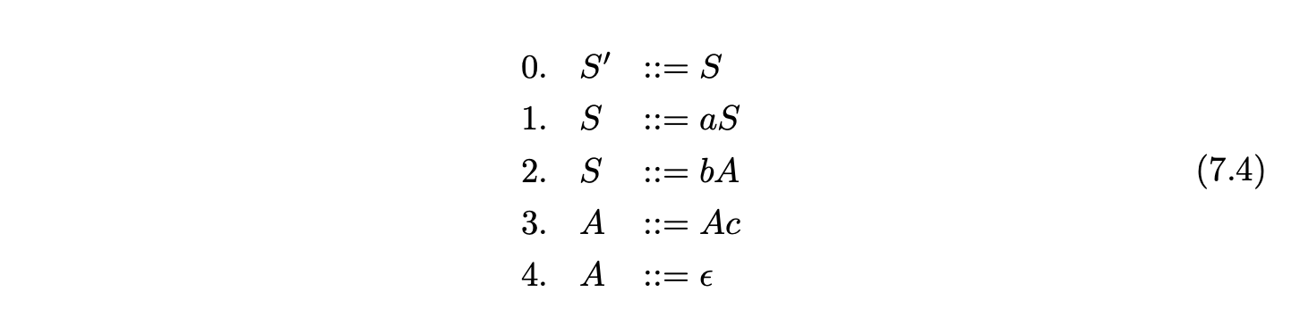
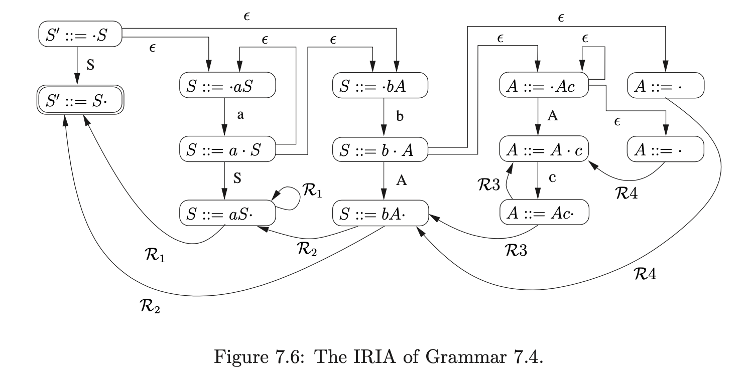
Since the rule \(S::=aS\) is right recursive, the state containing the item \((S::=a\cdot S)\) has \(\epsilon\)-edges going back to the states labelled by the items \((S::=\cdot aS)\) and \((S::=\cdot bA)\). We call the edges which are not created as a result of recursion primary edges.
Recall from Chapter 2 that if a grammar contains a non-terminal \(A\) such that \(A\stackrel{{+}}{{\Rightarrow}}\alpha A\beta\), where \(\alpha,\beta\neq\epsilon\), then the grammar contains self-embedding.
A formal definition of the IRIA construction algorithm, taken from [SJ], is given below. It has been proven in [SJ] that for a grammar, \(\Gamma\), that does not have any self embedded recursion, this algorithm will construct an IRIA that accepts precisely the sentential forms of \(\Gamma\).
IRIA construction algorithm
Given an augmented grammar \(\Gamma\) (without self embedded recursion) we construct an FA IRIA(\(\Gamma\)) as follows: Step 1: Create a node labelled \(S::=\cdot S\). Step 2: While there are nodes in the FA which are not marked as dealt with, carry out the following:
Pick a node \(K\) labelled \((X::=\mu\cdot\gamma)\) which is not marked as dealt with.
If \(\gamma\neq\epsilon\) then let \(\gamma=x\gamma^{\prime}\) where \(x\in\mathbf{N}\cup\mathbf{T}\), create a new node, \(M\), labelled \(X::=\mu x\cdot\gamma^{\prime}\), and add an arrow labelled \(x\) from \(K\) to \(M\). This arrow is defined to be a primary edge.
If \(x=Y\), where \(Y\) is a non-terminal, for each rule \(Y::=\delta\):
if there is a node \(L\), labelled \(Y::=\cdot\delta\), and a path \(\theta\) from \(L\) to \(K\) which consists of only primary edges and primary \(\epsilon\)-edges (\(\theta\) may be empty),add an arrow labelled \(\epsilon\) from \(K\) to \(L\). (This new edge is not a primary \(\epsilon\)-edge.)
if (a) does not hold, create a new node with label \(Y::=\cdot\delta\) and add an arrow labelled \(\epsilon\) from \(K\) to this new node. This is defined to be a primary \(\epsilon\)-edge.
Mark \(K\) as dealt with.
Step 3: Remove all the ‘dealt with’ marks from all nodes. Step 4: While there are nodes labelled \(Y::=\gamma\cdot\) that are not dealt with: pick a node \(K\) labelled \(X::=x_{1}\cdots x_{n}\cdot\) which is not marked as dealt with. Let \(Y::=\gamma\) be rule \(i\).
If \(X\neq S^{\prime}\) then find each node \(L\) labelled \(Z::=\delta\cdot X\rho\) such that there is a path labelled \((\epsilon,x_{1},\cdots,x_{n})\) from \(L\) to \(K\), then add an arrow labelled \(\mathcal{R}_{i}\) from \(K\) to the child of \(L\) labelled \(Z::=\delta X\cdot\rho\). Mark \(K\) as dealt with.
The new edge is called a reduction edge, and if the first (\(\epsilon\) labelled) edge of the corresponding path is a primary edge then this new edge is defined to be a primary reduction-edge.
Step 5: Mark the node labelled \(S^{\prime}::=\cdot S\) as the start node and mark the node labelled \(S^{\prime}::=S^{\cdot}\) as the accepting node.
7.3 Reducing non-determinism in the IRIA
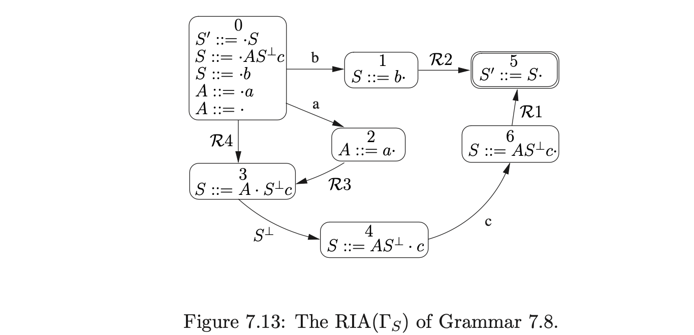
It is possible to use an IRIA to guide a parser though a derivation for a given string, but since the automaton is non-deterministic, the parser will encounter a choice of actions in certain states. This section presents the Reduction Incorporated Automaton (RIA), a more deterministic automaton than the IRIA which is constructed from the IRIA with the use of the subset construction algorithm.
There are four types of edges in an IRIA. Those labelled by the terminal or non-terminal symbols, the \(\epsilon\)-edges and the \(\mathcal{R}\)-edges. Once the \(\mathcal{R}\)-edges have been created in the IRIA, all the edges labelled with a non-terminal can be removed because they will not be traversed during a parse.
The \(\mathcal{R}\)-edges are used to locate the target state of a reduction. Since no terminal symbols are consumed during their traversal, it is tempting to treat them as \(\epsilon\)-edges during the subset construction. However, since many applications are required to produce a derivation of the input after a parse is complete, we cannot simply combine the states that can be reached by \(\mathcal{R}\)-edges that are labelled with different reductions. Instead we treat them in the same way that we treat the edges labelled by the terminal symbols.
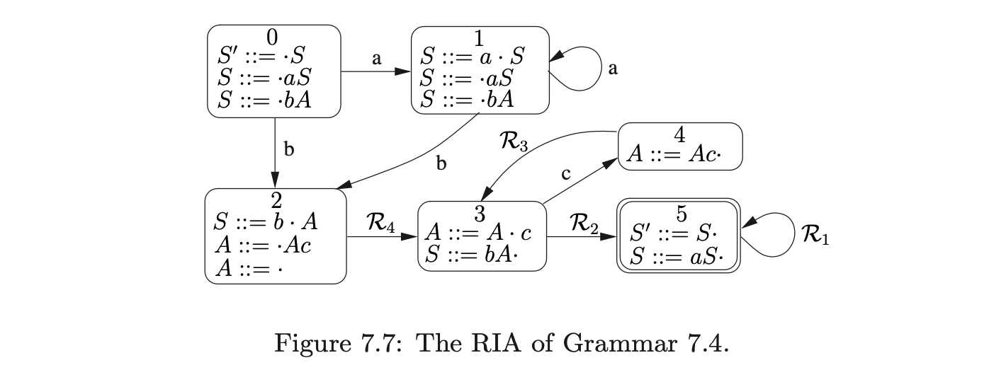
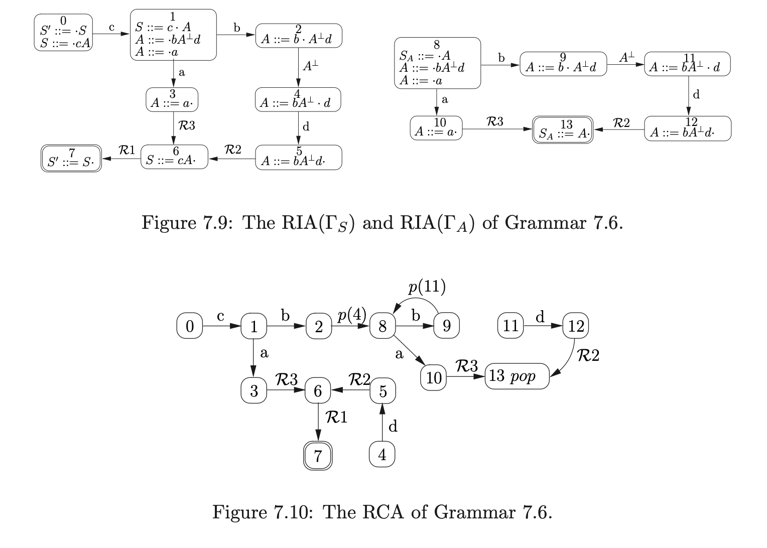
An RIA is constructed from an IRIA by removing the edges labelled by the non-terminal symbols and then performing the subset construction, treating the \(\mathcal{R}\)-edgesas non-empty edges. For example, the RIA in Figure 7.7 was constructed in this way from the IRIA in Figure 7.6.
7.4 Regular recognition
This section describes how to construct the PDA of a context-free grammar \(\Gamma\), that recognises strings in the language of \(\Gamma\) with a reduced amount of stack activity compared to GLR recognisers. The approach we take is an extension of the method described by Aycock and Horspool in [1]. The description of the algorithm is taken from [11, 12, 13].
7.4.1 Recursion call automata
Recall that a grammar has self embedded recursion if it contains a non-terminal \(A\), such that \(A\overset{\pm}{\Rightarrow}\alpha A\beta\) where both \(\alpha\) and \(\beta\neq\epsilon\). The structures expressed by self embedded recursion are inherently context-free and hence require a stack to be used to ensure that only valid strings are recognised.
We have already established that the amount of stack activity used during recognition can be reduced if we only use it to recognise these context-free structures. By locating the places that self embedded recursion occurs, we can build an automaton that only uses a stack at these places. This automaton is called the Recursion Call Automaton (RCA).
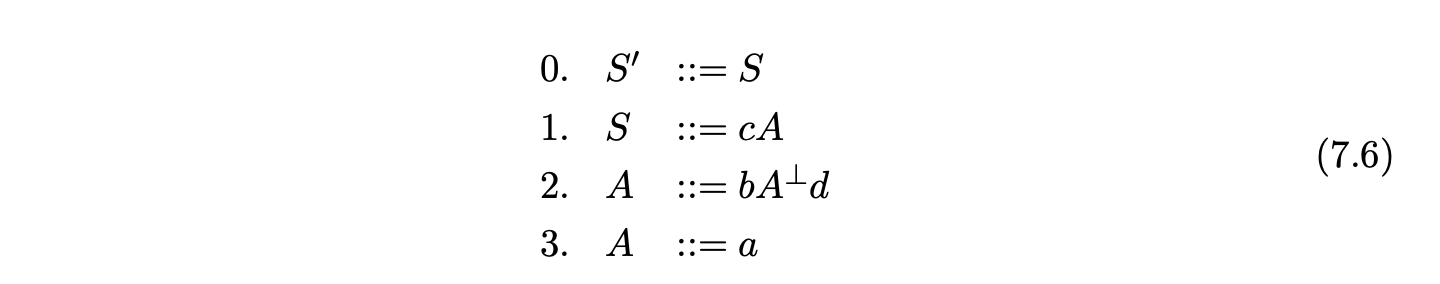
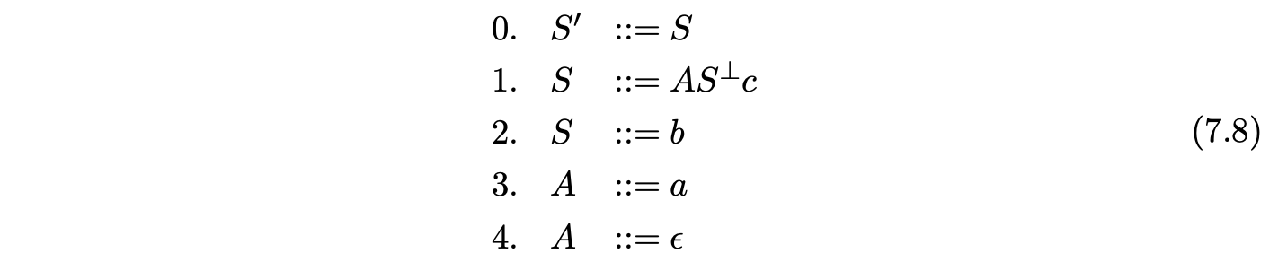
To construct an RCA, we first need to break any self embedded recursion in the grammar. We can achieve this by effectively ‘terminalising’ the non-terminals that appear in the self embedded production rules. We replace a non-terminal \(A\) in a production rule of the form \(X::=\alpha A\beta\), that has a derivation \(A\overset{\pm}{\Rightarrow}\alpha A\beta\), with the special terminal symbol \(A^{\perp}\), in a way that breaks the derivation. We call a grammar \(\Gamma\) that has had all instances of self embedded recursion removed in this way a derived grammar of \(\Gamma\) and denote it by \(\Gamma_{S}\).
In order to ensure that only the correct derivations of a string are produced (see Section 7.8), we require that any hidden-left recursion is also removed from a grammar before the RCA is constructed. We call the grammar that does not contain any self embedded recursion or hidden-left recursion, the derived parser grammar of \(\Gamma\).
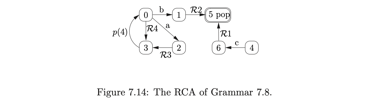
To build the RCA for a derived parser grammar of a context-free grammar \(\Gamma\), we build a separate RIA for each of the non-terminals defined in \(\Gamma\) and then link them together. For each of the non-terminals \(A\) (except \(S^{\prime}\) and \(S\)) we create a new rule \(S_{A}::=A\) in \(\Gamma\) and consider the grammar \(\Gamma_{A}\), which has the same rules as \(\Gamma\) but with the new start rule \(S_{A}::=A\). We then construct the IRIA and RIA for each \(\Gamma_{A}\). Once all of the separate, disjoint, RIA have been created, we link them together by removing an edge from a state \(h\) to a state \(k\) that is labelled \(A^{\perp}\) and add a new edge labelled \(p(k)\) from \(h\) to the start state of the RIA\((\Gamma_{A})\). In addition to this all the accept states of the RIA are labelled with a \(pop\). The start state and accepting states of the RCA are the same as the start and accept states of \(\Gamma_{S}\). For example consider Grammar 7.5.
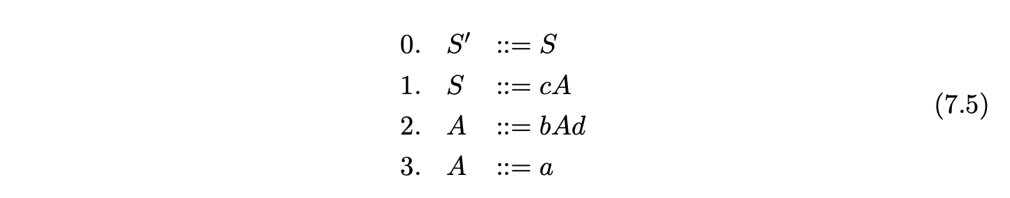
Since the non-terminal \(A\) is self embedded, our first step is to terminalise it to produce Grammar 7.6.
It has been proven in [SJ] that a string \(u\) is only in the language of a context-free grammar \(\Gamma\), if the RCA of \(\Gamma\) accepts \(u\).
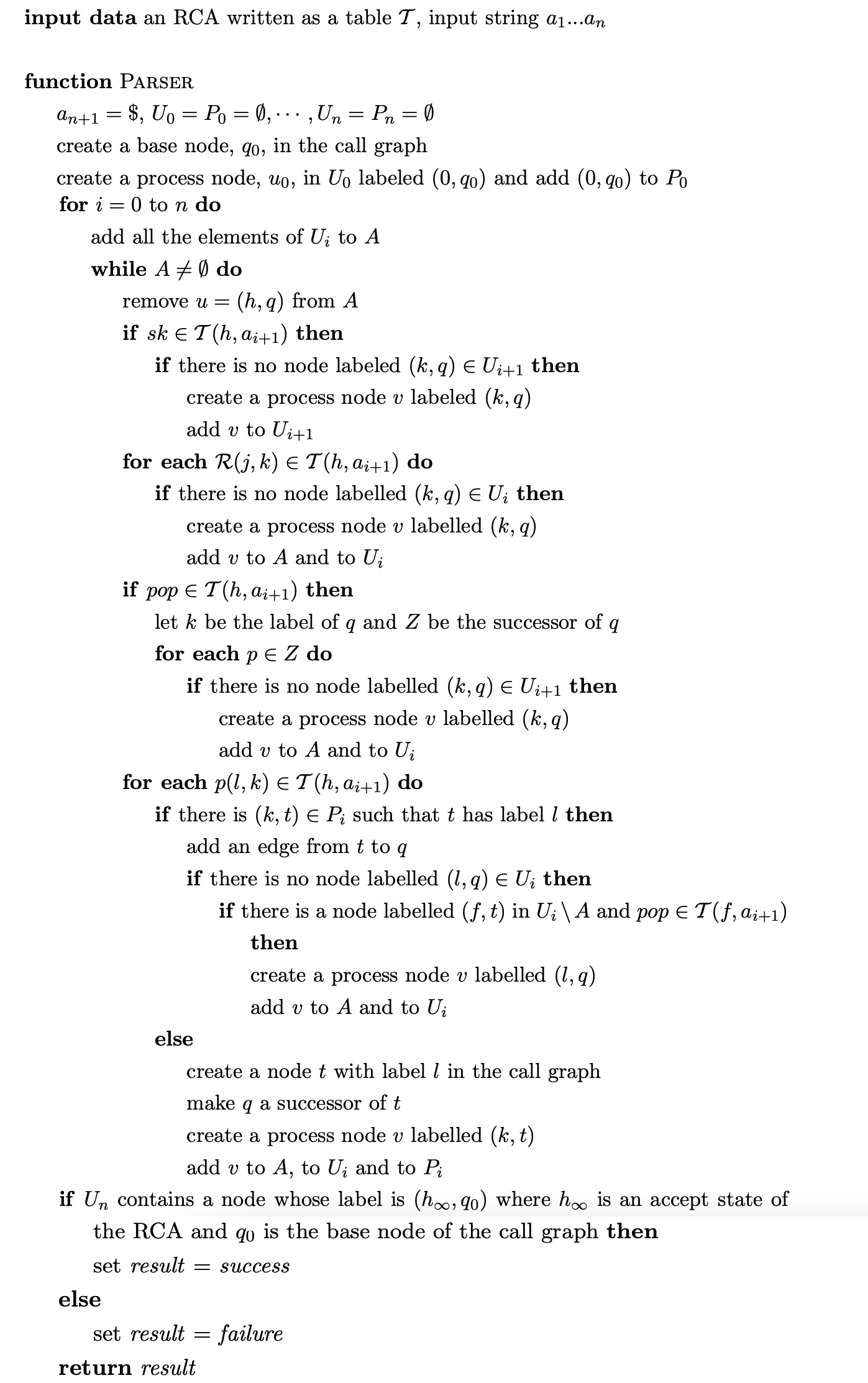
7.4.2 Parse table representation of RCA
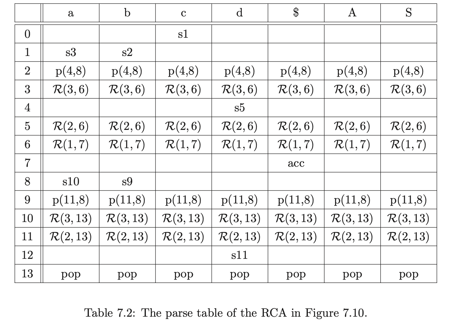
It is often convenient to represent an RCA(\(\Gamma\)) as a parse table, \(\mathcal{T}(\Gamma)\), where the rows of the table are labelled by the states of the automaton and the columns by the terminal symbols of \(\Gamma\) and the \(\$\) symbol. The parse table entries contain sets of actions corresponding to the actions associated with the states and edges of the RCA. For all edges from state \(h\) to state \(k\), if the edge is labelled by:
a terminal \(x\), then \(sk\) is in \(\mathcal{T}(h,x)\);
\(\mathcal{R}i\), then \(\mathcal{R}(i,k)\) is in all the columns of row \(h\) in \(\mathcal{T}\);
\(p(l)\), then \(p(l,k)\) is in all the columns of row \(h\) in \(\mathcal{T}\);
(In this version no lookahead is being employed.) In addition to the actions above, if a state \(h\) in the RCA is labelled \(pop\), then every column of state \(h\) in \(\mathcal{T}\) also contains a \(pop\) action. So for example, the parse table of the RCA in Figure 7.10 is shown in Table 7.2.
7.5 Generalised regular recognition
This section introduces the RIGLR recognition algorithm which finds a traversal of an RCA for a string \(a_{1}\ldots a_{n}\) if one exists. We begin by providing an informal description of the algorithm and then discuss some specific example grammars that need to be handled with care to ensure that a correct parse is achieved. There is a formal definition of the algorithm at the end of the section.
If there is a traversal, for a given string through an automaton, then that string is in the language defined by the automaton. A straightforward way of determining whether a string is in the language defined by an automaton is to traverse the automaton until all the input has been consumed and an accept state is reached. We can take this approach to traverse an RCA, but since it can be non-deterministic, there may be more than one traversal through the automaton that leads to an accept state for a given string. We are interested in finding all such paths, so we employ a breadth first search approach to follow all possible traversals when a choice arises.
A straightforward approach to traversing such a non-deterministic automaton is to maintain a set of states that can be reached by traversing the edges that do not consume any input symbols. In this case, it is the edges labelled by \(\mathcal{R}\). We achieve this by maintaining a set \(U_{i}\), where \(0\leq i\leq n\), during the parse of a string \(a_{1}\ldots a_{n}\). We begin by constructing the set \(U_{0}\) that contains the start state of the RCA and then add, in a similar way to the standard subset construction algorithm [1], all the states that can be reached by traversing the edges from the start state that do not consume any input symbols. When no more states can be added to the set \(U_{0}\) its construction is complete. We then proceed to create the set \(U_{i+1}\) from \(U_{i}\) by adding the states that can be reached by traversing an edge labelled with the current input symbol, \(a_{i+1}\), from each state in \(U_{i}\). An input string is accepted, if after consuming all input symbols the set \(U_{n}\) contains the RCA’s accept state.
This approach only works if the RCA’s underlying language does not contain any nested structures. If it does, then the RCA will contain push transitions labelled \(p(X)\), where \(X\) is a state number. When such an edge is traversed it is necessary to remember \(X\), since a state containing a pop action will eventually be reached that requires the parser to goto \(X\). It is tempting to store the return state in the set \(U\), along with the action’s source state, but the possibility of nested pushes and multiple paths caused by the non-determinism would make this approach inefficient.
We take the approach described by Aycock and Horspool in [1] and use a graph structure, similar to Tomita’s GSS (see Chapter 4), to record the return states of the push actions. We call this graph structure the Recursive Call Graph (RCG). When we encounter a push action during the traversal of the RCA with a return state \(l\) and a target state \(k\), we create a node \(q\) labelled \(l\) in the RCG and add the pair \((k,q)\) to the current set \(U_{i}\).
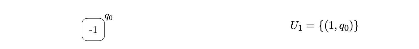
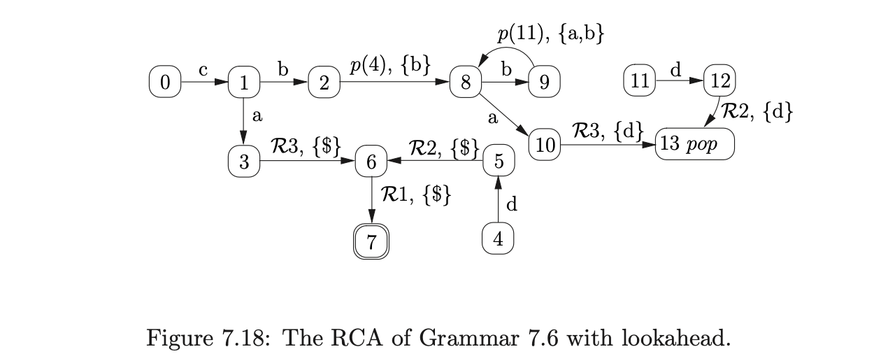
Consider Grammar 7.5 and the RCA constructed in Section 7.4. We parse the string \(cbad\) by first creating the base node, \(q_{0}\), of the RCG, labelled -1 (which is not the state number of any RCA state), and then add the element \((0,q_{0})\) to the set \(U_{0}\). Since the only edge that leaves state \(0\) is labelled by the terminal \(c\), which matches the first symbol on the input string, we move to state \(1\), and construct the new set \(U_{1}=\{(1,q_{0})\}\).
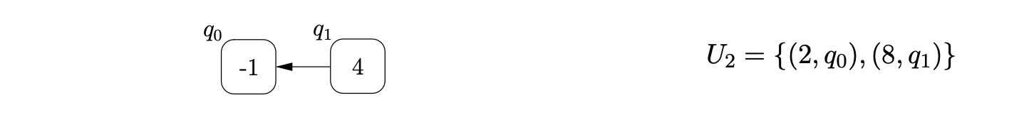
There are two edges from state 1, but since they are both labelled by terminal symbols we do not add anything to U1 in this step. The next input symbol is b, so we traverse the edge to state 2, create \(U2 = {(2, q_0)}\). Since there is an edge labelled \(p(4)\) from state 2, we create the new RCG node, q1, labelled 4 and then add (8,q1) to \(U2\).
The only edges leaving state 8 are labelled by terminal symbols, so we shift on the next input symbol which takes us from state 8, to state 10. We traverse the R-edges so that \(U3 = {(10,q1),(13,q1)}\). Since state 13 contains a pop action, we pop 4, which is the label of node q1 in the RCG, and add the element \((4,q0)\) to \(U3\).
At this point we have \(U3 = {(10,q_1),(13,q_1),(4,q_0)}\) and since there are no more edges that can be traversed without consuming any input symbols the third step of the algorithm is complete.
We then read the final symbol from the input string and traverse the edge labelled \(d\) to state 5 creating \(U_{4}=\{(5,q_{0})\}\). We traverse the \(\mathcal{R}\)-edges and construct \(U_{4}=\{(5,q_{0}),(6,q_{0}),(7,q_{0})\}\). Since the next input symbol is the end-of-string symbol, \(\$\), and \(U\) contains the element \((7,q_{0})\) which has the accept state of the RCA and the base node of the stack, the input \(cbad\) is accepted. Before we give the formal definition of the algorithm, we will discuss and show the construction of the RCG for three example grammars that can cause problems if they are not handled with care.
 It is necessary to traverse the reduction transition,
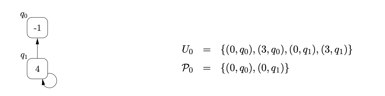
Example - ensuring all pop actions are done
When a pop action is performed by the algorithm on a node \(q\) with label \(h\) that has an edge to another node \(p\) in the RCG, the element \((h,p)\) is added to the set \(U_{i}\). If a new edge is added from node \(q\) to another node \(w\), in the same step of the algorithm, then we need to perform the \(pop\) action down this new edge. To ensure that this is done, when we add a new edge between \(q\) and \(w\), we check to see if \(U_{i}\) contains a process which results in a pop action being performed from \(q\). If such a process exists then we make sure that \(U_{i}\) contains the process \((h,w)\).
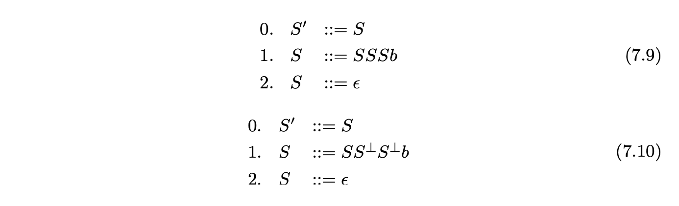
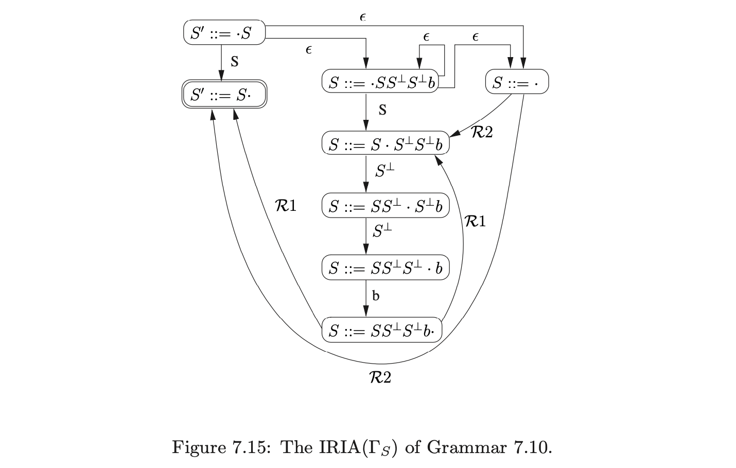
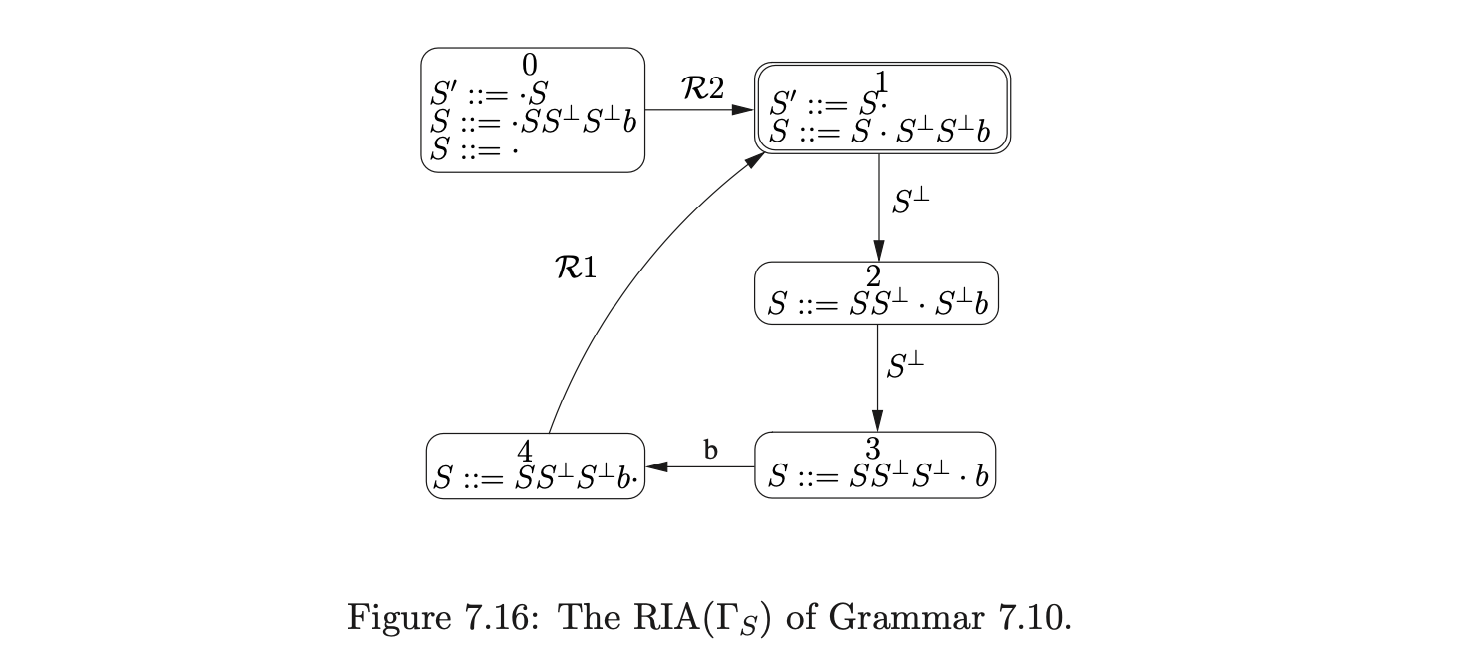
For example, consider Grammar 7.9, taken from [15], and the terminalised version, Grammar 7.10. The associated IRIA, RIA and RCA are shown in Figures 7.15, 7.16 and 7.17 respectively.
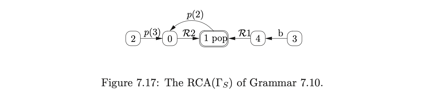
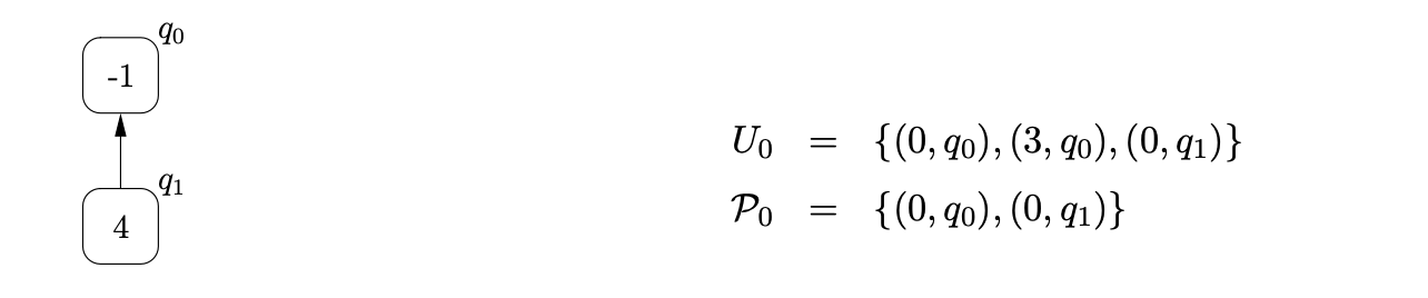
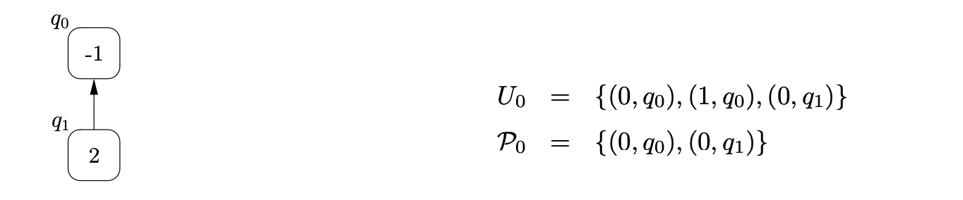
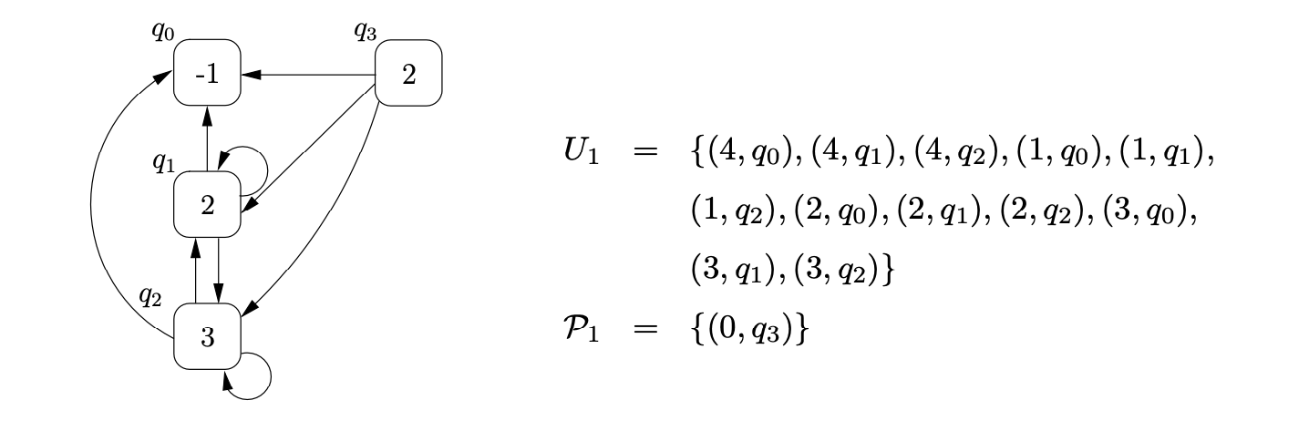
To parse the string \(b\) we begin by creating the base node of the RCG, \(q_{0}\), and add the process \((0,q_{0})\) to \(U_{0}\) and \(\mathcal{P}_{0}\). From state \(0\) in the RCA we move to state \(1\) on a transition labelled by \(\mathcal{R}2\) and add the process \((1,q_{0})\) to \(U_{0}\). Although state \(1\) contains a pop action, nothing is done since \(q_{0}\) does not have any children. We then traverse the edge labelled \(p(2)\) back to state \(0\), create the new RCG node, \(q_{1}\), with an edge to \(q_{0}\), and add \((0,q_{1})\) to \(U_{0}\) and \(\mathcal{P}_{0}\).
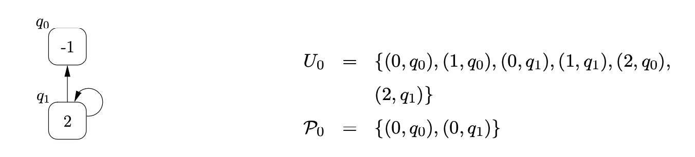
From state \(0\) we traverse the \(\mathcal{R}2\) edge to state \(1\) and add the process \((1,q_{1})\) to \(U_{0}\). At this point we can perform the pop action associated with state \(1\). We find the only child of \(q_{1}\), \(q_{0}\), and add \((2,q_{0})\) to \(U_{0}\). Traversing the edge labelled \(p(2)\) from state \(1\) to state \(0\), we first search \(\mathcal{P}_{0}\) to see if a node labelled \(2\) has been created during this step of the algorithm. Since \(q_{1}\) is in \(\mathcal{P}_{0}\) we re-use it and add a new edge from \(q_{1}\) to itself. However, the new edge on \(q_{1}\) has created a new path down which the previous pop action could be performed. It is therefore necessary to add \((2,q_{1})\) to \(U_{0}\). The current state of the RCG and the contents of the sets \(U_{0}\) and \(\mathcal{P}_{0}\) are shown below.
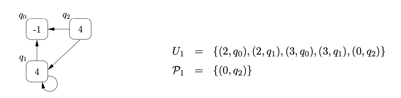
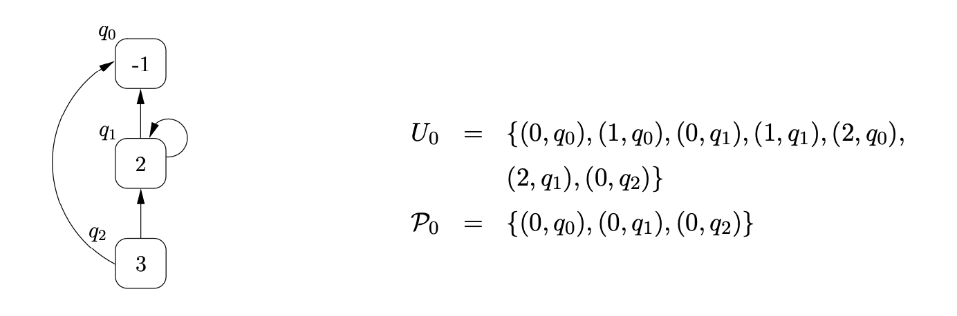
 We continue the parse by traversing the edge labelled with the push action, \(p(3)\), from state \(2\) to state \(0\), create the new RCG node, \(q_{2}\), labelled \(3\), with two edges. One edge goes from \(q_{2}\) to \(q_{0}\) and the other from \(q_{2}\) to \(q_{1}\). We also add \((0,q_{2})\) to \(U_{0}\) and \(\mathcal{P}_{0}\).
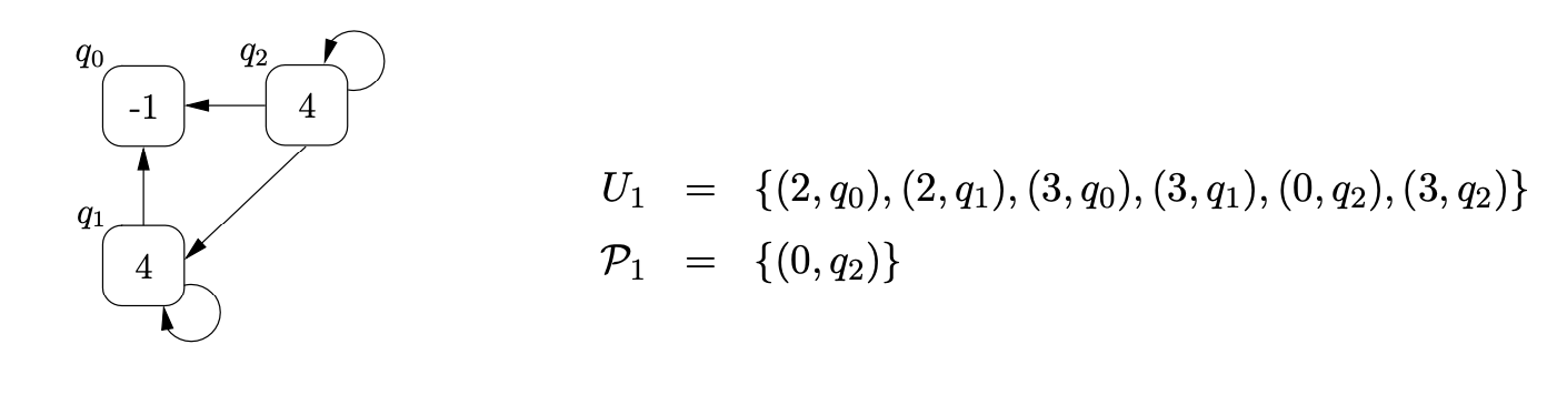
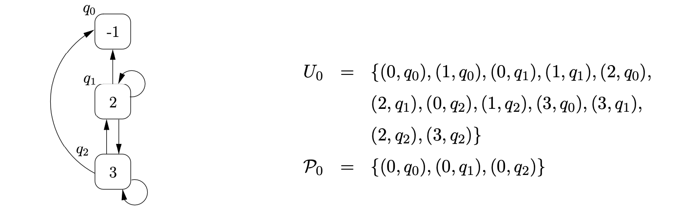
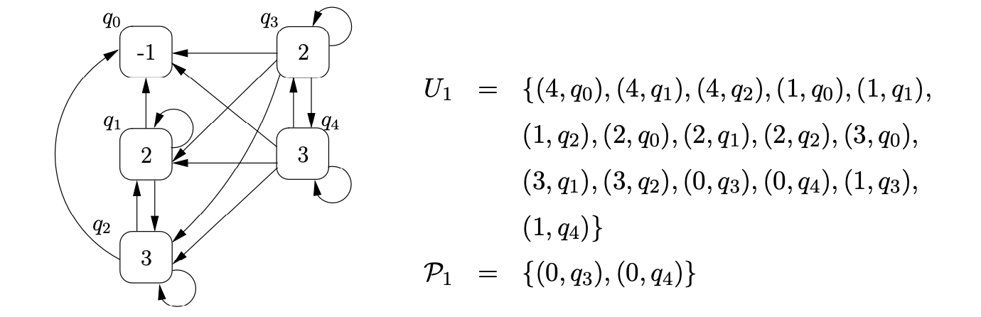
We then traverse the \(\mathcal{R}2\) edge to state \(1\), add \((1,q_{2})\) to \(U_{0}\) and proceed to perform the pop on \(q_{2}\). We find the children of \(q_{2}\), \(q_{0}\) and \(q_{1}\), and add \((3,q_{0})\) and \((3,q_{1})\) to \(U_{0}\). Traversing the edge labelled \(p(2)\) from state \(1\) to state \(0\), we re-use \(q_{1}\) and add a new edge from \(q_{1}\) to \(q_{2}\). This new edge has created a new path down which the previous pop action could be performed so we add \((2,q_{2})\) to \(U_{0}\). When we perform the push transition, \(p3\), from state \(2\) of the RCA (as a result of \((2,q_{2})\) being added to \(U_{0}\)) we create a new looping edge for \(q_{2}\). Since a pop we already performed can also be performed down this new edge, we also add \((3,q_{2})\) to \(U_{0}\). That completes the first step of the algorithm. The current state of the RCG and the contents of the sets \(U_{0}\) and \(\mathcal{P}_{0}\) are shown below.
We then read the next input symbol \(b\), construct the new set \(U_{1}=\{(4,q_{0}),(4,q_{1}),(4,q_{2})\}\) and set \(\mathcal{P}_{1}=\emptyset\). We traverse the \(\mathcal{R}1\) edge to state \(1\), add \((1,q_{0}),(1,q_{1}),(1,q_{2})\) to \(U_{1}\) and then perform the associated pop action for \(q_{1}\) and \(q_{2}\). We add \((2,q_{0}),(2,q_{1}),(2,q_{2})\) and \((3,q_{0}),(3,q_{1}),(3,q_{2})\) to \(U_{1}\). Traversing the push transition, \(p2\), from state \(1\), we create a new RCG node, \(q_{3}\), labelled \(2\) and add edges from it to the nodes \(q_{0},q_{1}\) and \(q_{2}\).
 Continuing the parse in this way results in the creation of the final RCG shown below.
Since all the input has been consumed and the process \((1,q_{0})\) is in \(U_{1}\), where state \(1\) is the accepting state of the RCA and \(q_{0}\) is the RCG’s base node, the input string \(b\) is accepted.
RIGLR recogniser
7.6 Reducing the non-determinism in the RCA
We can reduce the amount of non-determinism in the RCA by adding lookahead sets to the reduce, push and pop actions. The lookahead sets are calculated for the reduce and push actions by traversing the \(\mathcal{R}\)-edges and push edges until a state is reached that has edges leaving it that are labelled by terminal symbols. These terminals are added to the lookahead set of all the edges on the path to the state. If the target state is an accept state then the lookahead set also includes the \(\$\) symbol.
Since the pop action is part of a state, we label the state with a lookahead set which is calculated by finding the lookahead sets of the states that can be reached when the pop action is performed. These states are the targets of the edges labelled by the terminalised symbols in the RIA.
The implementation used in PAT does not incorporate lookahead because the RCA are produced by GTB and GTB does not, at present, construct RCA with lookahead.
Reducing the number of processes in each \(U_{i}\)
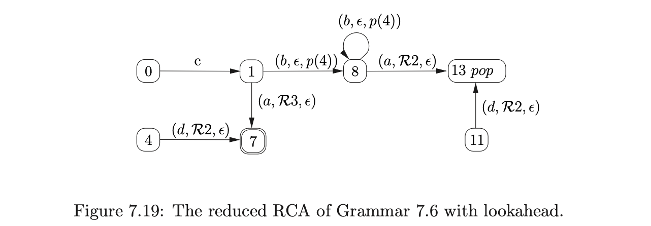
The number of processes added to \(U_{i}\) at each step of the RIGLR algorithm can be very large. An approach to reduce both the size of the RCA and the number of processes added at each step of the algorithm is presented in [1]. It involves ‘pre-compiling’ and then combining sequences of actions in the RCA. The basic principle is to combine a preceding terminal that can be shifted, with all \(\mathcal{R}\)-edges, and/or a following push edge. For example, consider the pre-compiled RCA shown in Figure 7.19 that has been constructed from the RCA in Figure 7.18.
 Although this approach can reduce the size of the RCA, if we want to incorporate lookahead into the RCA, we have to use two symbols of lookahead. This will increase the size of the parse table and hence also the size of the parser. More seriously, if all possible sequences of reductions are composed then the number of new edges in the RCA can be increased from \(O(k)\) to \(O(2^{k+1})\). An example of this is given in [15].
However, limited composition has been proposed in [15] that guarantees not to increase the size of the RCA. The implementation used in PAT does not incorporate this technique to reduce the size of the sets \(U_{i}\).
Although this approach can reduce the size of the RCA, if we want to incorporate lookahead into the RCA, we have to use two symbols of lookahead. This will increase the size of the parse table and hence also the size of the parser. More seriously, if all possible sequences of reductions are composed then the number of new edges in the RCA can be increased from \(O(k)\) to \(O(2^{k+1})\). An example of this is given in [15].
However, limited composition has been proposed in [15] that guarantees not to increase the size of the RCA. The implementation used in PAT does not incorporate this technique to reduce the size of the sets \(U_{i}\).
7.8 Generalised regular parsing
This section introduces the RIGLR parsing algorithm which attempts to find a traversal of an RCA for a string \(a_{1}\ldots a_{n}\) and constructs a syntactic representation of the string. We begin by providing an informal description of how to build a derivation tree using an example for which the RCA is deterministic. Then we present an efficient way of representing multiple derivations. There is a formal definition of the algorithm at the end of the section.
7.8.1 Constructing derivation trees
We can build a derivation tree for an input string \(a_{1}\ldots a_{n}\) during a parse by maintaining a sequence of tree nodes, \(u_{1},\ldots,u_{p}\), constructed at each step of the algorithm. When an edge labelled with a terminal symbol, \(a\), is traversed, we create a parse tree node and append it to the sequence of nodes created thus far. When a \(\mathcal{R}_{i}\) edge is traversed, where rule \(i\) is \(A::=x_{1}\ldots x_{k}\), we remove nodes, \(u_{p-k+1},\ldots,u_{p}\), from the sequence, create a new node labelled \(A\), with children \(u_{p-k+1},\cdots,u_{p}\), and append the new node to the end of the sequence. No tree nodes need to be created for the push and pop transitions of the RCA.
Figure 7.19: The reduced RCA of Grammar 7.6 with lookahead.
For example, consider the parse of the string \(cbad\) for Grammar 7.6 and its associated RCA shown in Figure 7.10 (see page 7.10). We shall maintain the parse tree root nodes in the sequence \(\mathcal{W}\).
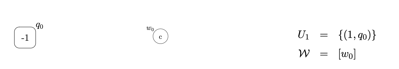
We begin the parse, as usual, by creating the base node of the RCG and adding the element \((0,q_{0})\) to the set \(U_{0}\) and \(\mathcal{P}_{0}\). We read the first input symbol \(c\), traverse the edge from state \(0\) to state \(1\), create the first parse tree node, \(w_{0}\), labelled c and construct the set \(U_{1}=\{(1,q_{0})\}\).
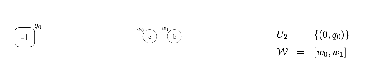
We continue the parse by reading the next input symbol, \(b\), traversing the edge from state \(1\), labelled \(b\), to state \(2\), create the new parse tree node, \(w_{1}\), and construct the set \(U_{2}=\{(2,q_{0})\}\).
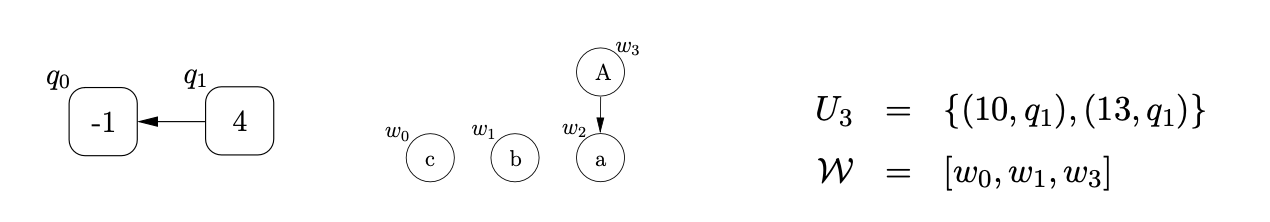
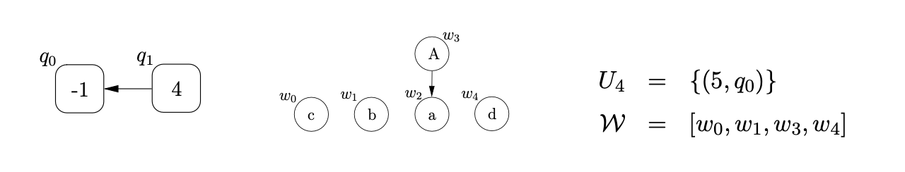
The next transition from state \(2\) is labelled by the push action \(p(4)\), so we create the new RCG node, \(q_{1}\), labelled \(4\) and add \((8,q_{1})\) to \(U_{2}\). (Recall that no nodes are created in the parse tree as a result of the traversal of a push edge in the RCA.) We then read the third input symbol, \(a\), traverse the edge to state \(10\), create the parse tree node \(w_{2}\), labelled \(a\), and construct the set \(U_{3}=\{(10,q_{1})\}\). From state \(10\), there is a reduction transition labelled \(\mathcal{R}_{3}\) for rule \(A::=a\). We traverse the edge to state \(13\) and then create the new parse tree node, \(w_{3}\), labelled \(A\). Since rule \(3\) has a right hand side of length \(1\), we remove the last element from the sequence \(\mathcal{W}\) and use it to label the child node of \(w_{3}\). We then add the new root node to the set \(\mathcal{W}\), and add \((13,q_{1})\) to \(U_{3}\).
Since state \(13\) contains a pop action, we find the child, \(q_{0}\), of the RCG node \(q_{1}\), and add \((4,q_{0})\) to \(U_{3}\). We read the final input symbol \(d\), create the new parse tree node, \(w_{4}\), and construct \(U_{4}\) as shown below.
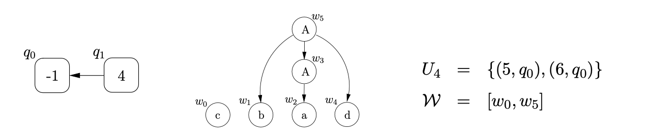
We then traverse the reduction transition, \(\mathcal{R}_{2}\) from state 5. Rule 2 is \(A::=bAd\), so we create the new node, \(w_{5}\), labelled \(A\), remove the last three parse tree nodes from the sequence \(\mathcal{W}\) and add them to \(w_{5}\) as its children. We also add \(w_{5}\) to \(\mathcal{W}\) and \((6,q_{0})\) to \(U_{4}\).
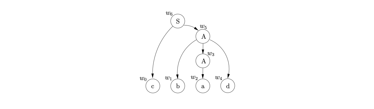
We then traverse the reduction transition, \(\mathcal{R}1\) from state 6 to state 7. Rule 1 is \(S::=cA\), so we create the new node \(w_{6}\), labelled S, remove the final two parse tree nodes from the sequence \(\mathcal{W}\), and add them to \(w_{6}\) as its children. Since we have consumed all the input and the process \((7,q_{0})\) is in \(U_{4}\), where 7 is the RCA’s accepting state and \(q_{0}\) is the base node of the RCG, the input string \(cbad\) is accepted by the parser. The final parse tree is shown below.
In the above example, the RCA is deterministic and hence there is only one derivation tree for the input string. Recall that some parses can have an exponential, or even infinite, number of derivations for a given string. We use Tomita’s SPPF representation of multiple parse trees to reduce the amount of space necessary to represent all parse trees. The next section discusses three different approaches that can be used to construct an SPPF of a parse using an RCA.
7.8.2 Constructing an SPPF
There are several different approaches that can be taken to construct an SPPF during a parse of the RIGLR algorithm. A straightforward technique is to store a sequence of SPPF nodes that correspond to the roots of the sub-trees that have been constructed so far with each process \((k,q)\). However, since it is possible to reach a state in the RCA by traversing more than one path, this approach can significantly increase the number of processes constructed at each step of the algorithm [11].
An alternative approach is to merge the processes that share the same call graph nodes, so as to limit the number of processes that need to be created. Instead of storing the sequence of SPPF nodes directly in a process, we can represent the sequences of SPPF nodes in an SPPF node graph - a type of graph structured stack - and replace the sequence of nodes in a process by a single SPPF node graph node.
Unfortunately, as is shown in [15], this approach leads to spurious derivations being created in the SPPF for certain parses. Another disadvantage of using the SPPF node graph is that the structure needs to be traversed in order to construct the final SPPF, which is likely to affect the order of the parsing algorithm.
A solution proposed in [15] is to use special SPPF pointer nodes that point to sequences of SPPF nodes within the SPPF. To prevent the spurious derivations from being created, the edges in the call graph are labelled with these special SPPF pointer nodes. This provides a way of only associating the correct derivation sequences with their associated processes.
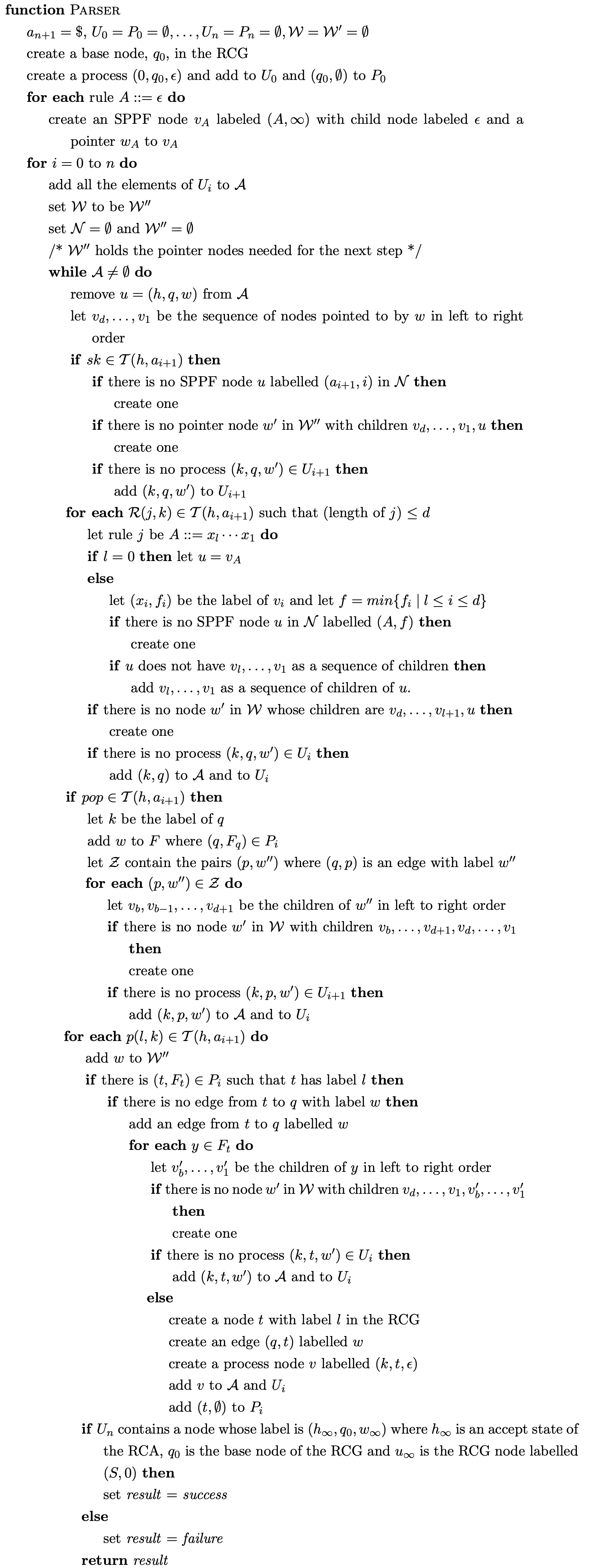
Another problem with the construction of the SPPF is caused if an existing node in the RCG, that has already had a pop applied, has a new edge added to it as a result of a push action. In Example 7.5.1 we show how the recognition algorithm deals with such cases - when a new edge is added to an existing node, all processes in \(U_{i}\) are checked to see if a pop was applied. Unfortunately, this approach does not simply work for the parser because we need to ensure that the correct tree is constructed for any pops that are re-applied. Thus we use the set \(\mathcal{P}_{i}\) to store the SPPF nodes that are associated to a pop’s reduction path. When a pop is performed, we add the sequence of SPPF nodes to a set \(F\) and store it in the pair \((q,F)\) in \(\mathcal{P}_{i}\). When a push action for a process \((h,q,w)\) is performed, we check to see if \(\mathcal{P}_{i}\) contains an element of the form \((q,F)\). If it does, then a pop has already been performed from state \(q\). We use the sequences of SPPF nodes in \(F\) to add the required new processes to \(U_{i}\) that will cause the pops to be re-applied for the correct reduction paths.
Before presenting the formal description of the RIGLR parser we shall work through an example of the construction of an SPPF during a parse using the final approach discussed above. For example, consider the parse of the string \(abcc\), with Grammar 7.8 and RCA shown in Figure 7.14 on page 7.14.
In addition to the sets \(U_{i}\) and \(\mathcal{P}_{i}\) we maintain two additional sets during parsing. The sets \(\mathcal{N}\) and \(\mathcal{W}\) are used to store the SPPF nodes and special pointer nodes, respectively, that are created at the current step of the algorithm. Recall from Chapter 4 that nodes in an SPPF that are labelled by the same non-terminal and derive the same portion of the input string can be merged. To achieve this efficiently, we label each SPPF node with a pair \((x,j)\), where \(j\) is an integer representing the start position within the input string that the yield of the sub-graph \((x,j)\) derives. (The set \(\mathcal{N}\) is used to reduce the number of SPPF nodes that need to searched to find the ones that can be packed. It also allows SPPF nodes to be labelled by the pair \((x,j)\) since all nodes in the set will have been constructed at the current step of the algorithm.)
Furthermore, the SPPF of a specific \(\epsilon\)-rule can be shared throughout a parse whenever a reduction is done for that rule. To avoid creating redundant instances of an \(\epsilon\)-SPPF we shall create all \(\epsilon\)-SPPF’s at the start of the algorithm and use them whenever necessary.
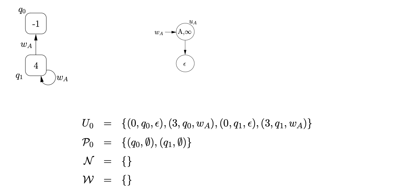
Since Grammar 7.8 contains the \(\epsilon\)-rule \(A::=\epsilon\), we build the tree, \(u_{A}\), with pointer \(w_{A}\). We begin the parse by creating the base node of the RCG and adding the process \((0,q_{0},\epsilon)\) to \(U_{i}\).
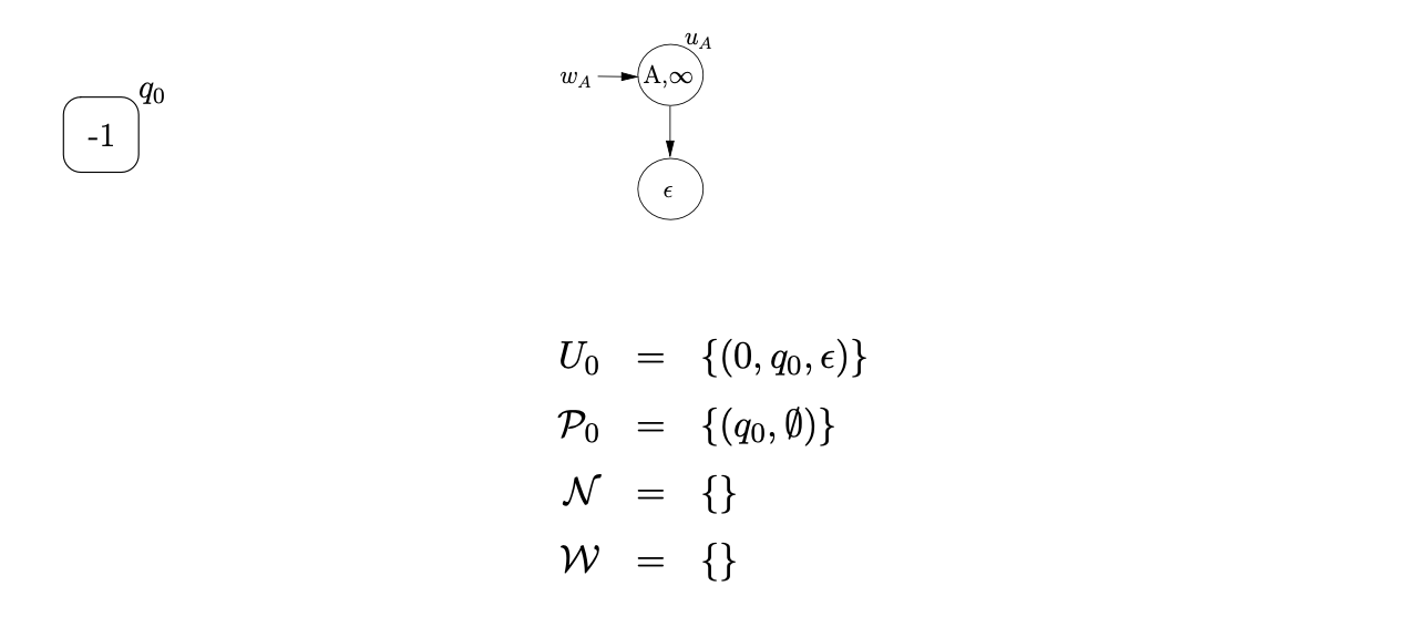
We then traverse the edge labelled \(\mathcal{R} 4\) from state 0 to state 3 , add the process \(\left(3, q_{0}, w_{A}\right)\) to \(U_{0}\) and then traverse the push edge labelled p(4) back to state 0 . The push action results in the new RCG node, \(q_{1}\), with an edge labelled \(w_{A}\) to \(q_{0}\), being created and \(\left(0, q_{1}, \epsilon\right)\) being added to \(U_{0}\) and \(\left(q_{1}, \emptyset\right)\) to \(\mathcal{P}_{0}\). The SPPF is not modified. We traverse the \(\mathcal{R} 4\) edge again for process \(\left(0, q_{1}, \epsilon\right)\), add \(\left(3, q_{1}, w_{A}\right)\) to \(U_{0}\) and then traverse the push transition \(p(4)\). This results in a new edge, labelled \(w_{A}\), being added to the RCG as a loop on \(q_{1}\).
 We continue the parse by reading the next input symbol, a, and then traverse the edge from state 0 to state 2 . We create the new \(SPPF\) node, \(u_{1}\), labelled (a, 0), add a pointer node \(w_{1}\) to \(u_{1}\) and construct \(U_{1}=\left\{\left(2, q_{0}, w_{1}\right),\left(2, q_{1}, w_{1}\right)\right\}\). For each of these processes we traverse the edge labelled \(\mathcal{R} 3\) to state 3 , create the SPPF node, \(u_{2}\), labelled (A, 0) with pointer node \(w_{2}\), and add the processes \(\left(3, q_{0}, w_{2}\right)\) and \(\left(3, q_{1}, w_{2}\right)\) to \(U_{1}\). We add \(u_{1}\) as the child of \(u_{2}\) since we created the new SPPF node from the processes \(\left(2, q_{0}, w_{1}\right),\left(2, q_{1}, w_{1}\right)\). From state 3 we traverse the edge p(4) to state 0 , create the new RCG node, \(q_{2}\), and two edges labelled \(w_{2}\) from \(q_{2}\) to \(q_{0}\) and \(q_{1}\). The process \(\left(0, q_{2}, \epsilon\right)\) is also added to \(U_{1}\) and \(\left(q_{2}, \emptyset\right)\) to \(\mathcal{P}\).
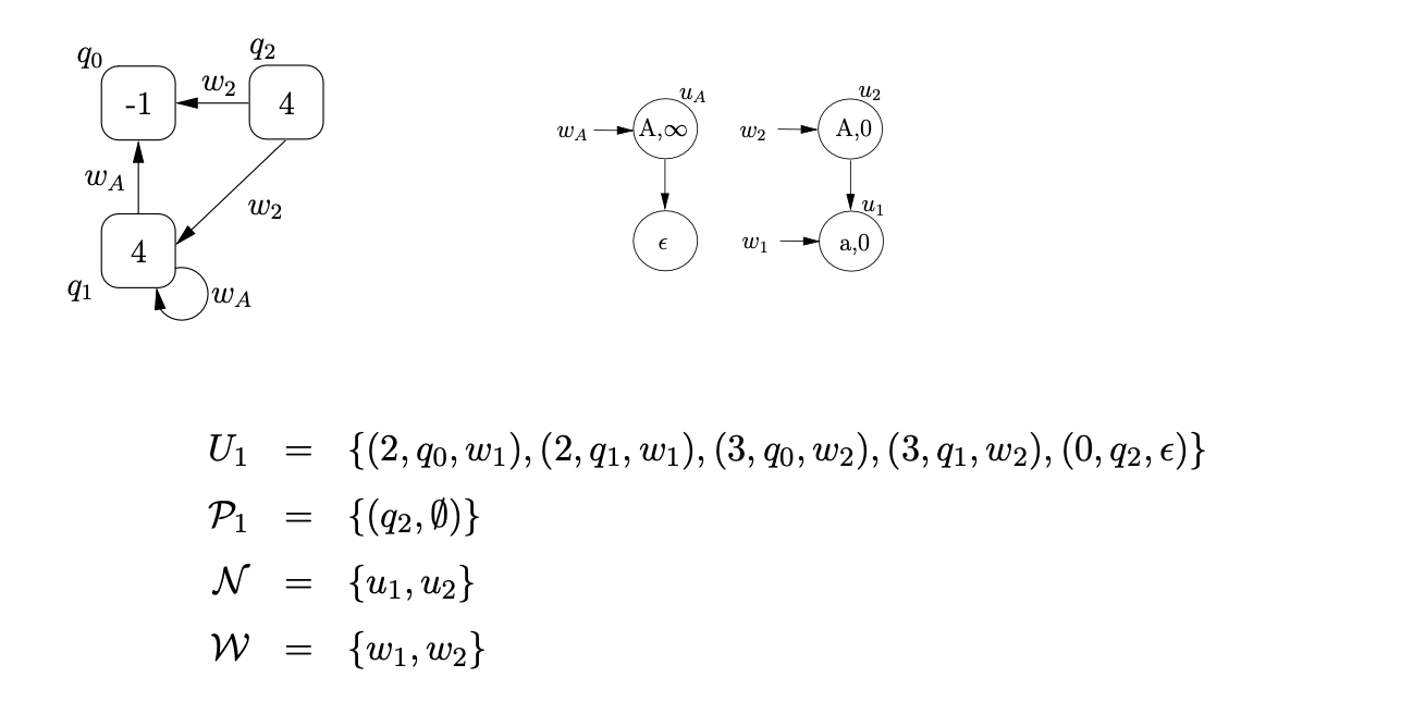
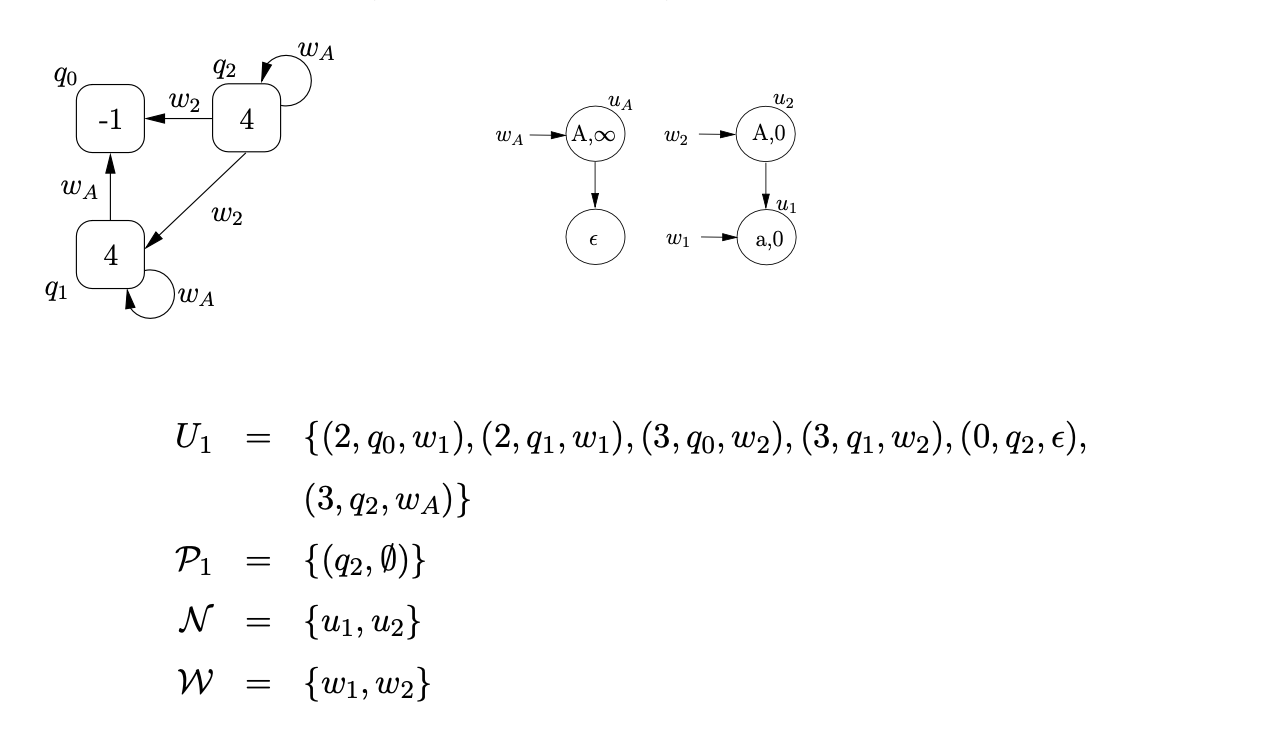
We then traverse the edge \(\mathcal{R} 4\) from state 0 to state 3 for process \(\left(0, q_{2}, \epsilon\right)\), followed by the push transition back to state 0 . This results in the process \(\left(3, q_{2}, w_{A}\right)\) being added to \(U_{1}\), and the edge labelled \(w_{A}\) being added to the RCG from \(q_{2}\) to itself.
 Traversing the edge labelled b from state 0 , we create the new SPPF node, \(u_{3}\), labelled (b, 1), with pointer node \(w_{3}\), and construct \(U_{2}=\left\{\left(1, q_{2}, w_{3}\right)\right\}\). We then traverse the \mathcal{R} 2 edge to state 5 , create the SPPF node \(u_{4}\), labelled (S, 1), with pointer node \(w_{4}\) and update the relevant sets as shown below.
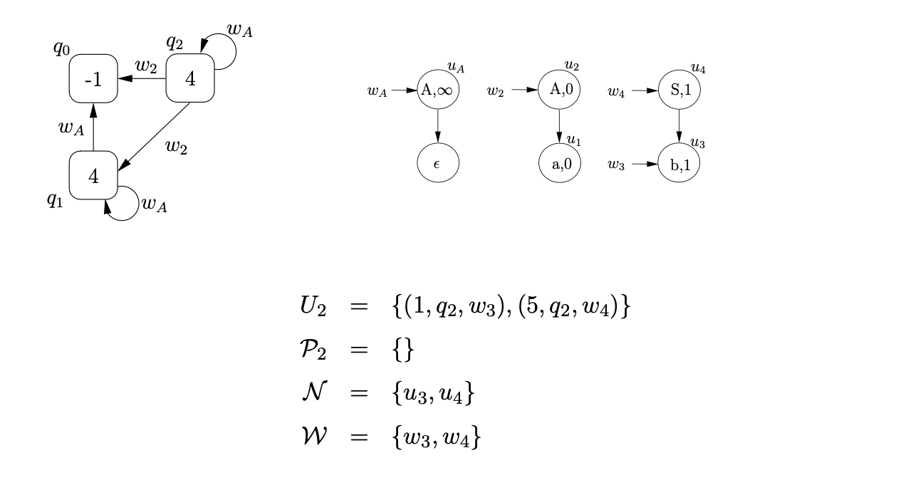 Performing the pop action associated with state 5, for process \((5,q_{2},w_{4})\), we first find the children of \(q_{2}\), \(q_{0},q_{1},q_{2}\). Then we create two new pointer nodes \(w_{5}\) and \(w_{6}\), with edges to the children of the pointers of the popped edges in the RCG and \(w_{4}\). For each of the new pointers we also add the processes \((4,q_{0},w_{5}),(4,q_{1},w_{5})\) and \((4,q_{2},w_{6})\) to \(U_{2}\).
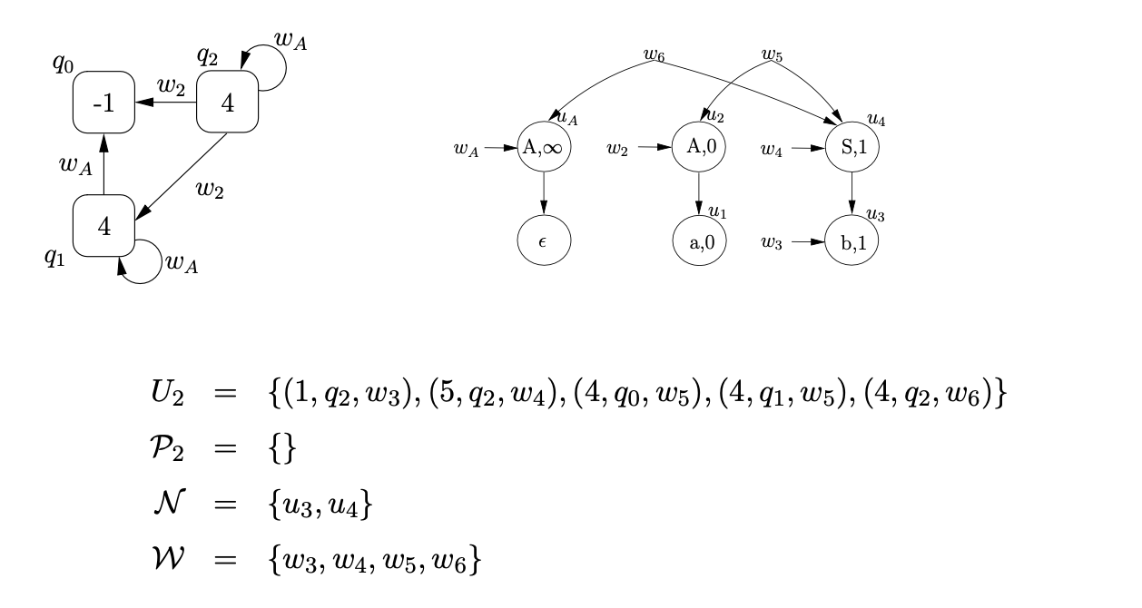
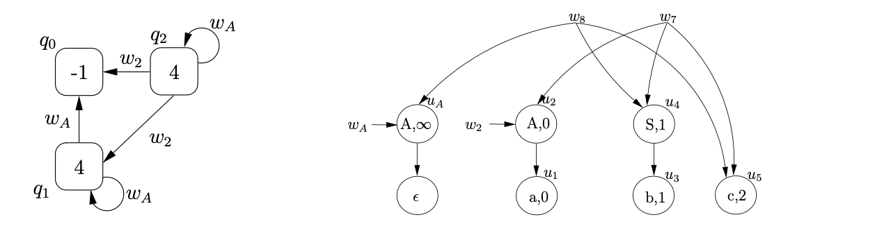
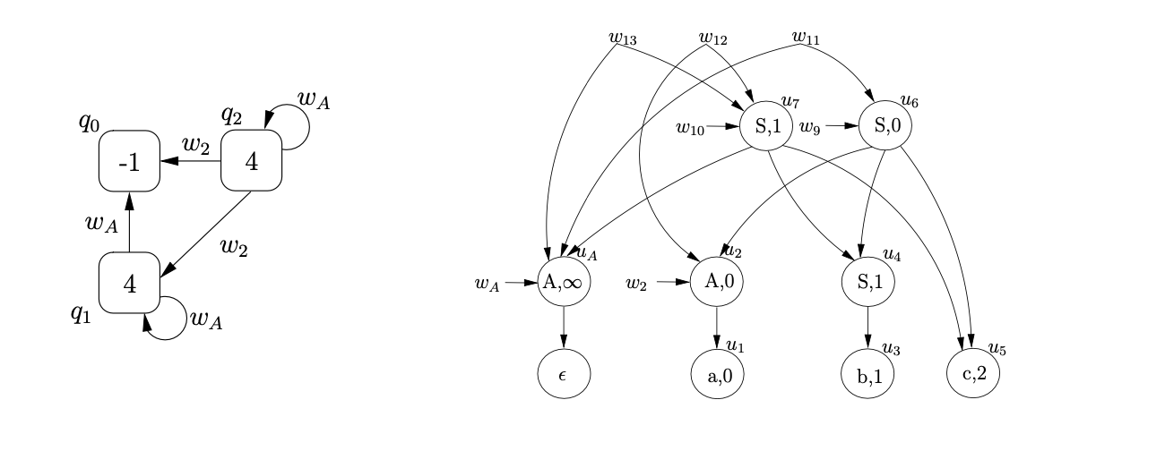
We continue the parse by reading the next input symbol \(c\) and then create the new SPPF node, \(u_{5}\), labelled \((c,3)\), with two pointer nodes \(w_{7}\) and \(w_{8}\). We construct \(U_{3}=\{(6,q_{0},w_{7}),(6,q_{1},w_{7}),(6,q_{2},w_{8})\}\), \(\mathcal{N}=\{u_{5}\}\) and \(\mathcal{W}=\{w_{7},w_{8}\}\).
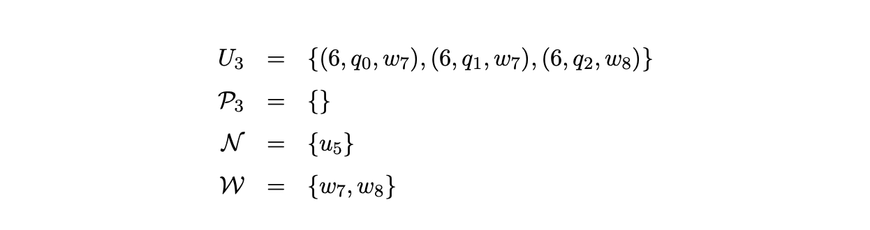
From state 6 we the traverse the \(\mathcal{R}1\) edge to state 5 and create two new SPP nodes \(u_{9}\) and \(u_{10}\), labelled \((S,0)\) and \((S,1)\), respectively. The state of the parser is shown below.
 Performing the pop action associated with state 5 , for processes \(\left(5, q_{1}, w_{9}\right)\) and \(\left(5, q_{2}, w_{10}\right)\), we first find the children of \(q_{1}\) and \(q_{2}, q_{0}, q_{1}\) and \(q_{0}, q_{1}, q_{2}\). Then we create three new pointer nodes \(w_{11}, w_{12}\) and \(w_{13}\), with edges to the children of the pointers of the popped edges in the RCG and \(w_{9}\) and \(w_{10}\) respectively. The state of the parser after the pop is complete is shown below.
Next we read the final input symbol \(c\), create \(u_{8}\) labelled \((c,3)\) and three new pointer nodes \(w_{14},w_{15}\) and \(w_{16}\) in the SPPF. We traverse the edge from state 4 to state 6 and construct \(U_{4}\).
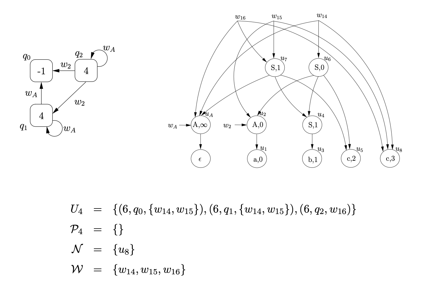
For each of the processes in \(U_{4}\) we traverse the \(\mathcal{R} 1\) edge from state 6 in the RCA. For processes \(\left(6, q_{0},\left\{w_{14}, w_{15}\right\}\right)\) and \(\left(6, q_{1},\left\{w_{14}, w_{15}\right\}\right)\) we create a new SPPF node, \(u_{9}\), labelled (S, 0), with a pointer node \(w_{17}\). Since there are two pointer nodes \(w_{14}\) and \(w_{15}\) associated with both processes, we create two packing nodes below \(u_{9}\), one with edges to the children of \(w_{14}\) and the other with edges to the children of \(w_{15}\). For \(\left(6, q_{2}, w_{16}\right)\) we create the new SPPF node, \(u_{10}\), labelled (S, 1) with pointer node \(w_{18}\) and edges to the children of \(w_{16}\).
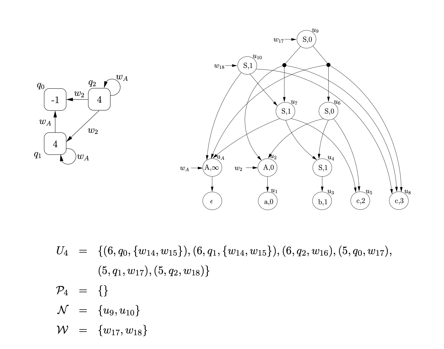
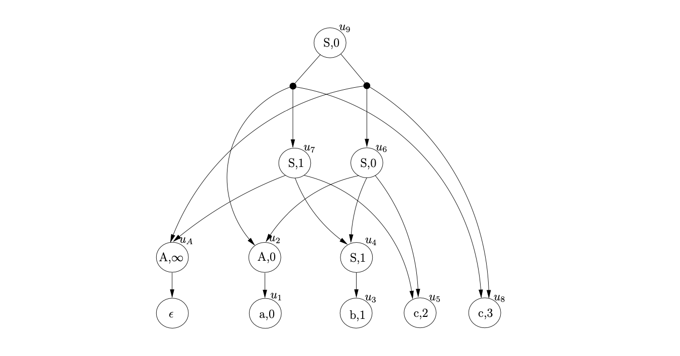
Since the process \((5,q_{0},w_{17})\) is in \(U_{4}\), and state \(5\) is the accept state of the RCA, and \(q_{0}\) is the base node of the RCG, the string \(abcc\) is accepted. We make the root node of the SPPF the node pointed to by \(w_{17}\). The final SPPF, without any pointer nodes is shown below.
RIGLR parser
7.9 Summary
In this chapter we examined the role of the stack in bottom-up parsers and described how to construct the automata that can be used by the RIGLR recognition and parsing algorithms to parse with less stack activity than other GLR parsing techniques. Chapter 10 contains the results of several experiments that highlight the performance of the RIGLR recognition algorithm compared to the other GLR algorithms.