2. Recognition and parsing¶

In order to execute programs, computers need to be able to analyse and translate programming languages. In general, programming languages are simpler than human languages, but many of the principles involved in studying them are similar.

The compilation process as a whole has been meticulously studied for a long time. However, writing a correct and efficient parser by hand is still a difficult task. Although tools exist that can automatically generate parsers from a grammar specification, limitations with the techniques mean that they often fail.

The early high level programming languages, like $FORTRAN$, were developed with expressibility rather than parsing efficiency in mind. Some language constructs turned out to be difficult to parse efficiently, but without a proper understanding of the reasons behind this inefficiency, a solution was difficult to come by. The subsequent work on formal language theory by Chomsky provided a solid theoretical base for language development.

The field of research that investigates languages, grammars and parsing is called formal language theory. This chapter provides a brief overview of language classification as defined by Chomsky [Cho56] and introduces the formal definitions and basic concepts that underpin programming language parsing. We discuss general top-down and bottom-up parsing and the standard deterministic LR parsing technique.

2.1 Languages and grammars¶

In formal language theory a language is considered to be a set of sentences. A sentence consists of a sequence of words that are concatenations of a number of symbols from a finite alphabet. A finite language can be defined by providing an enumeration of the sentences it contains. However, many languages are infinite and attempting to enumerate their contents would be a fruitless exercise. A more useful approach is to provide a set of rules that describe the structure, or syntax, of the language. These rules, collectively known as a grammar, can then be used to generate or recognisesyntactically correct sentences.

The work pioneered by Chomsky in the late 1950’s formalised the notion of a grammar as a generative device of a language[1]. He developed four types of grammars and classified them by the structures they are able to define. This famous categorisation, known as the Chomsky hierarchy, is shown in Table 2.1. Each class of language can be specified by a particular type of grammar and recognised by a particular type of formal machine. The automata in the right hand column of the table are the machines that accept the strings of the associated language.

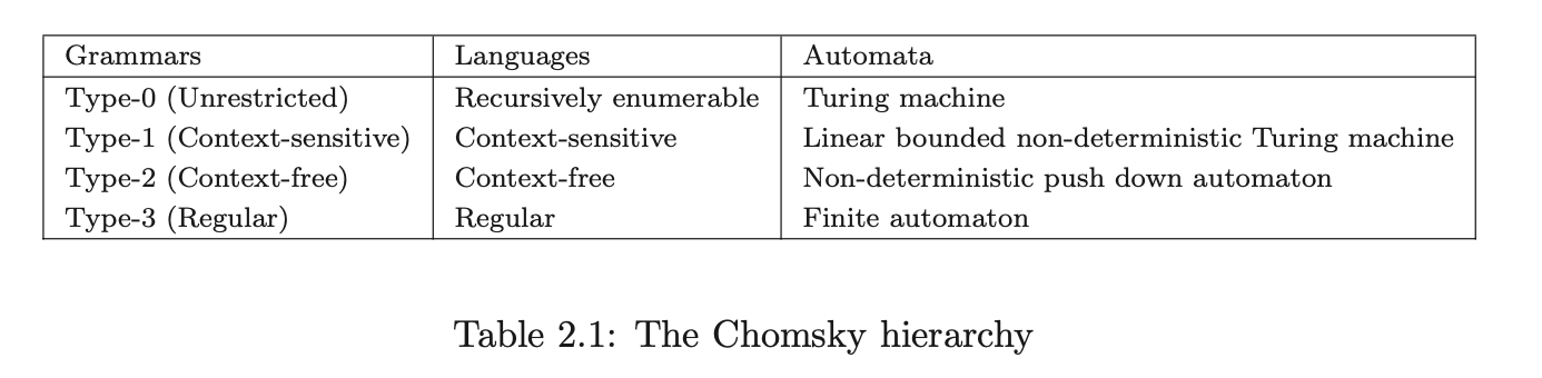
The grammars towards the bottom of the hierarchy define the languages with the simplest structure. The rules of a regular grammar are severely restricted and as a result, are only capable of defining simple languages. For example, they cannot generate languages in which parentheses must occur in matched pairs. Despite the limited nature of the regular languages, the corresponding finite automata play an important role in the recognition of the more powerful context-free languages.

The languages defined by context-free grammars are less confined by the restrictions imposed upon their grammar rules. In addition to expressing all the regular languages, they can also define recursively nested structures, common in many programming languages. As a result, the context-free grammars are often used to define the structure of modern programming languages and their automata form the basis of many classes of corresponding recognition and parsing tools.

Certain structural dependencies cannot be expressed by a context-free grammar alone. The context-sensitive grammars define the languages whose structure depends upon their surrounding context. Although attempts have been made to use the context-sensitive grammars to define natural languages, see for example [14], the resulting grammars tend to be very difficult to understand and use. In a similar way, although the recursively enumerable languages, generated by the type-0 grammars, are the most powerful in the hierarchy, their complicated structure means that they are usually only of theoretical interest.

2.2 Context-free grammars¶

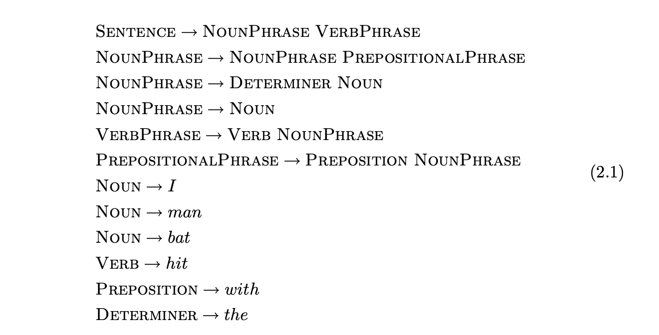
At the core of a context-free grammar is a finite set of rules. Each rule defines a set of sequences of symbols that it can generate. There are two types of symbols in a context-free grammar; the terminals, which are the symbols, letters or words, of the language and the non-terminals which can be thought of as variables - they constitute the left hand sides of the rules. An example of a context-free grammar for a subset of the English language is given in Grammar 2.1. The non-terminals are shown as the upper case words and the terminals as the lower case words.

2.2.1 Generating sentences¶

We generate strings from other strings using the grammar rules by taking a string and replacing a non-terminal with the right hand side of one of its rules. So for example, from the string

we can generate

by replacing the non-terminal VerbPhrase. We often write this as and call it a derivation step.

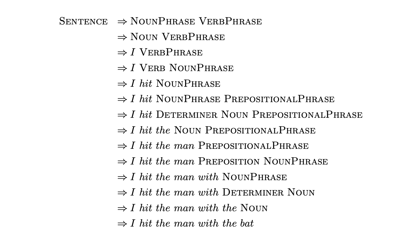
We are interested in the set $L(A)$ of all strings, that contain only terminals, that can be generated from a non-terminal $A$. This is called the language of $A$. One of the non-terminals will be designated as the start symbol and the language generated by this non-terminal is called the language of the grammar. For example, the sentence_I hit the man with a bat_ can be generated from the non-terminal SENTENCE in Grammar 2.1 in the following way:

A sequence of derivation steps is called a derivation.
The basic idea is to use a grammar to define our chosen programming language.

Then given some source code we need to determine if it is a valid program, ie a sentence in the language of the grammar. This can be achieved by finding a derivation of the program. The construction of derivations is referred to as parsing, or syntax analysis.

2.2.2 Backus Naur form¶

At about the same time as Chomsky was investigating the use of formal grammars to capture the key properties of human languages, similar ideas were being used to describe the syntax of the Algol programming language $\left[\mathrm{BWvW}^{+} 60\right]$. Backus Naur Form (also known as Backus Normal Form or BNF) is the notation developed to describe Algol and it was later shown that languages defined by BNF are equivalent to context-free grammars [GR62]. Because of its more convenient notation, BNF has continued to be used to define programming languages.

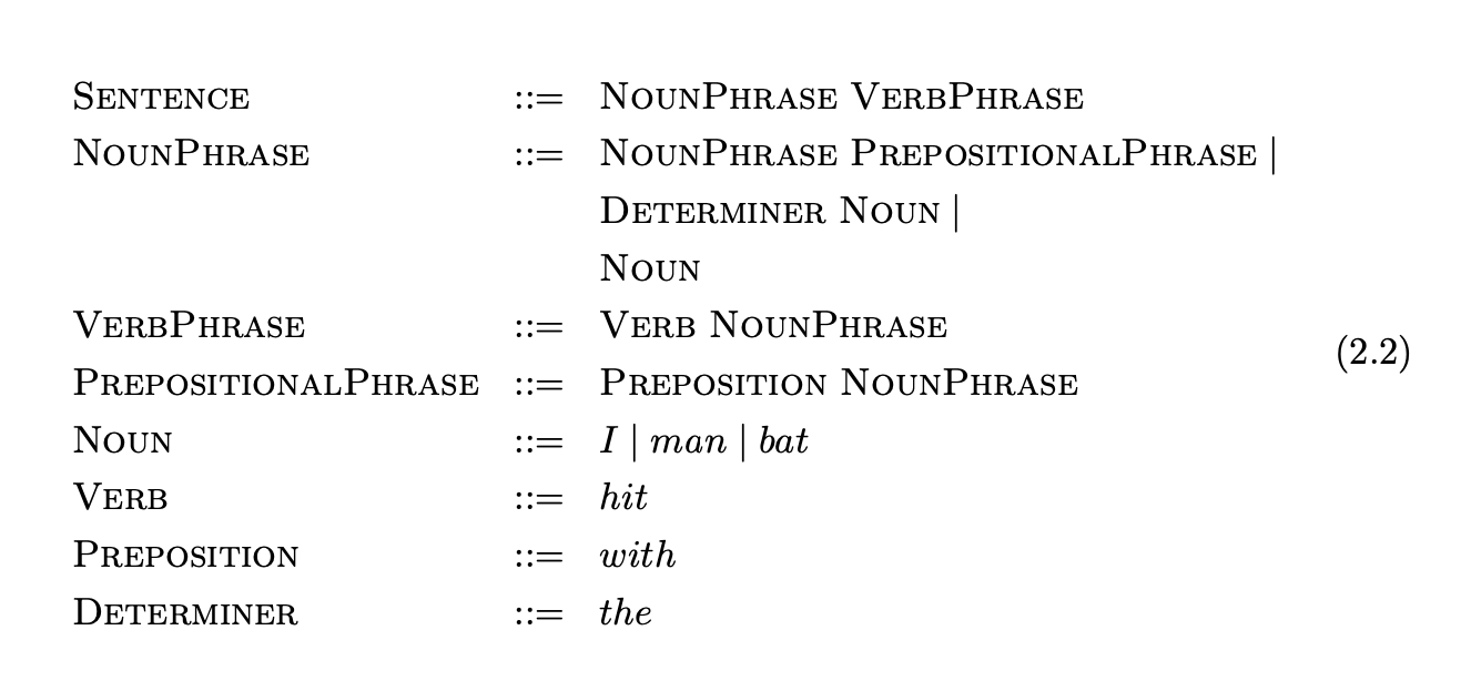
In BNF the non-terminals that declare a rule are separated from the body of the rule by ::= instead of the $\rightarrow$ symbol. In addition to this, a rule can define a choice of sequences with the use of the $|$ symbol. So for example, Grammar 2.2 is the BNF representation of Grammar 2.1.

We shall use the BNF notation to define all of the context-free grammars in the remainder of this thesis. In addition to this, we shall maintain the following convention when discussing context-free grammars: lower case characters near the front of the alphabet, digits and symbols like $+$, represent terminals; upper case characters near the front of the alphabet represent non-terminals; lower case characters near the end of the alphabet represent strings of terminals; upper case characters near the end of the alphabet represent strings of either terminals or non-terminals; lower case Greek characters represent strings of terminals and/or non-terminals.

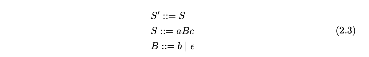
We define a context-free grammar formally as a 4-tuple $\langle\mathbf{N},\mathbf{T},\mathbf{S},\mathbf{P}\rangle$, where $\mathbf{N}$ and $\mathbf{T}$ are disjoint finite sets of grammar symbols, called non-terminals and terminals respectively; $\mathbf{S}\in\mathbf{N}$ is the special start symbol; $\mathbf{P}$ is the finite set of production rules of the form $A::=\beta$, where $A\in\mathbf{N}$ and $\beta$ is the string of symbols from $(\mathbf{N}\cup\mathbf{T})^{*}$. The production rule $S::=\alpha$ where $S\in\mathbf{S}$ is called the grammar’s start symbol. We may augment a grammar with the new non-terminal, $S^{\prime}$, that does not appear on the right hand side of any other production rule. The empty string is represented by the $\epsilon$ symbol. For example consider Grammar 2.3 which defines the language $\{ac,abc\}$.

The replacement of a single non-terminal in a sequence of terminals and non-terminals is called a derivation step and is represented by the $\Rightarrow$ symbol. The application of a number of derivation steps is called a derivation. We use the $\stackrel{*}{\Rightarrow}$ symbol to represent a derivation consisting of zero or more steps and the $\stackrel{{+}}{{\Rightarrow}}$ symbol for derivations of one or more steps. Any string $\alpha$ such that $S \stackrel{*}{\Rightarrow} \alpha$ is called a sentential form and a sentential form that contains only terminals is called a sentence. A non-terminal that derives the empty string is called nullable. If $A::=\epsilon$ then $\alpha A\beta\Rightarrow\alpha\beta$.

We call rules of the form $A::=\alpha\beta$ where $\beta\stackrel{{*}}{{=}}\epsilon$ right nullable rules. A grammar that contains a non-terminal $A$, such that $A\stackrel{{+}}{{\Rightarrow}}\alpha A\beta$, where $\alpha,\beta\neq\epsilon$, is said to contain self-embedding.

Since there is often a choice of non-terminals to replace in each derivation step, one of two approaches is usually taken; either the leftmost or the rightmost non-terminal is always replaced. The former approach achieves a leftmost derivation whereas the latter produces a rightmost derivation. The derivation in Section 2.2 is a leftmost derivation.

2.2.3 Recognition and parsing¶

An important aspect of the study of context-free grammars is the recognition of the sentences of their languages. It turns out that given any context-free grammar there is a Push Down Automaton (PDA) that accepts precisely the language of the grammar. Tools that take a string and determine whether or not it is a sentence are called recognisers.

In addition to implementing a recogniser, many applications that use context-free grammars also want to know the syntactic structure of any strings that are recognised. Since the rules of a grammar reflect the syntactic structure of a language, we can build up a syntactic representation of a recognised string by recording the rules used in a derivation. Tools that construct some form of syntactic representation of a string are called parsers.

2.2.4 Parse trees¶

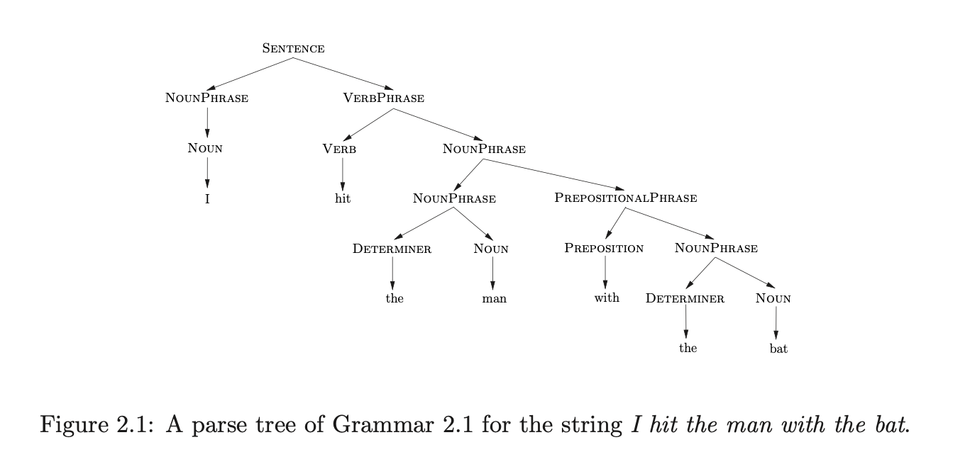
A useful way of representing the structure of a derivation is with a parse tree. A parse tree is a rooted tree with terminal symbols of the sentence appearing as leaf nodes and non-terminals as the interior nodes. If an interior node is labelled with the non-terminal $A$ then its children are labelled $A_{1},...,A_{j}$, where the rule $A::=A_{1}...A_{j}$ has been used at the corresponding point in the derivation. The root of a parse tree is labelled by the start symbol of the associated grammar and its yield is defined to be the sequence of terminals that label its leaves. Figure 2.1 is a parse tree representing the derivation of the sentence I hit the man with a bat for Grammar 2.1.

2.3 Parsing context-free grammars¶

The aim of a parser is to determine if it is possible to derive a sentence from a context-free grammar whilst also building a representation of the grammatical structure of the sentence. There are two common approaches to building a parse tree, top-down and bottom-up. This section presents the top-down and bottom-up parsing approaches.

Top-down parsing¶

A top-down parser attempts to derive a sentence by performing a sequence of derivation steps from the start rule of the grammar. It gets its name from the order in which the nodes in the parse tree are constructed during the parsing process; each node is created before its children.

Top-down parsers are usually implemented to produce leftmost derivations and are sometimes called predictive parsers because of the way they ‘predict’ the rules to use in a derivation. To parse a string we begin with the start symbol and predict the right hand side of the start rule. If the first symbol on the right hand side of the predicted rule is a terminal that matches the symbol on the input, then we read the next input symbol and move on to the next symbol of the rule. If it is a non-terminal then we predict the right hand side of the rule it defines.

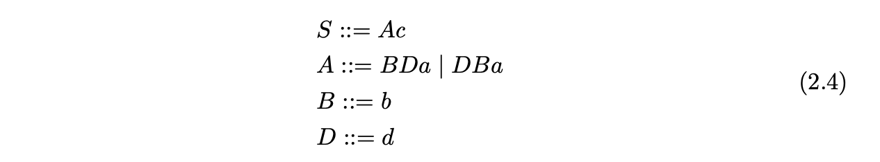
For example consider the following top-down parse of the string bdac for Grammar 2.4.

The start symbol of the grammar is defined to be $S$, so we begin by creating the root of the parse tree and labeling it $S$.

The right hand side of the start rule is made up of two symbols so the new sentential form generated is $Ac$. We create two new nodes, labelled $A$ and $c$ respectively, and add them as children of the root node.

At this point we are looking at the first symbol of the sentential form $Ac$. Since $A$ is a non-terminal, we need to predict the right hand side of the rule it defines. However, the production rule for $A$ has two alternates, $BDa$ and $DBa$, so we are required to pick one. If the first alternate is selected, then the parse tree shown below is constructed.

The new sentential form is $BDac$, so we continue by predicting the non-terminal $B$ and create the following parse tree.

We then match the symbol $b$ in the sentential form $bDac$ with the next input symbol and continue to predict the non-terminal $D$. This results in the parse tree below being constructed. The only symbols in the sentential form that have not yet been parsed are the terminals $dac$. A successful parse is completed once all of these symbols are matched to the remaining input string.

Perhaps the most popular implementation of the top-down approach to parsing is the recursive descent technique. Recursive descent parsers define a parse function for each production rule of the grammar - when a non-terminal is to be matched, the parse function for that non-terminal is called. As a result recursive descent parsers are relatively straightforward to implement and their structure closely reflects the structure of the grammar.

This approach to parsing can run into problems when there is a choice of alternates to be used in a derivation. For example, in the above parse if we had picked the rule $DBa$ instead of $BDa$ then the parse would have failed.

We could backtrack to the point that a choice was made and choose a different alternative, but this approach can result in exponential costs and in certain cases may not even terminate. A particular problem is caused by grammars with left recursive rules.

Recursive grammars

A grammar has $\textit{left (or right)}$ recursion if it contains a non-terminal $A$ and a derivation $A \stackrel{+}{\Rightarrow} \alpha A \beta$ where $\alpha \stackrel{*}{\Rightarrow} \epsilon (or \beta \stackrel{*}{\Rightarrow} \epsilon )$. If \alpha \neq \epsilon( or \beta \neq \epsilon) then the recursion is referred to as hidden.

Unfortunately, the standard recursive descent parsers, and most parsers that produce leftmost derivations, cannot easily parse left recursive grammars. In the case of a left recursive rule like $A::=Ab$, the parse function for $A$ will repeatedly call itself without matching any input.

Although left recursion can be mechanically removed from a grammar [AU73], the removal process alters the structure of the grammar and hence the structure of the parse tree.

2.3.2 Bottom-up parsing¶

A bottom-up parser attempts to build up a derivation in reverse, effectively deriving the start symbol from the string that is parsed. Its name refers to the order in which the nodes of the parse tree are constructed; the leaf nodes at the bottom are created first, followed by the interior nodes and then finally the root of the tree.

It is natural for the implementation of a bottom-up parser to produce a right-most derivation. A string is parsed by shifting (reading) a number of its symbols until a string of symbols is found that matches the right hand side of a rule. The portion of the sentential form that matches the right hand side of a production rule is called a handle. Once the handle is found, the substring in the sentential form is reduced (replaced) by the non-terminal on the left hand side of the rule. For each of the terminal symbols shifted, a leaf node in the parse tree is constructed. When a reduction is performed, a new intermediate node is created and the nodes labelled by the symbols in the handle are added to it as children. A string is successfully parsed when a node labelled by the grammar’s start symbol is created in the parse tree and the sentential form only contains the grammar’s start symbol.

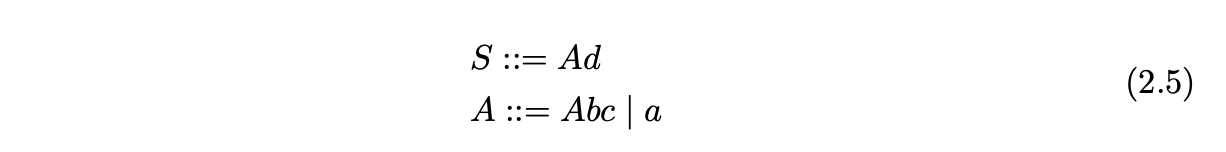
For example, consider Grammar 2.5 and the parse tree constructed for a bottom-up parse of the string $abcd$.

We begin by shifting the first symbol from the input string and create the node labelled $a$ in the parse tree.

Since there is a rule $A::=a$ in the grammar, we can use it to reduce the sentential form $a$ to $A$. We create the new intermediate node in the parse tree labelled $A$ and make it the parent of the existing node labelled $a$.

We continue by shifting the next two input symbols to produce the sentential form $Abc$. At this point we can reduce the whole of the sentential form to $A$ using the rule $A::=Abc$. We create the new node labelled $A$ as a parent of the nodes labelled $A$, $b$ and $c$ in the parse tree.

Once the final input symbol is shifted, we can reduce the substring $Ad$ in the sentential form to the start symbol $S$ and create the root node of the parse tree to complete the parse.

Bottom-up parsers that are implemented to perform these shift and reduce actions are often referred to as shift-reduce parsers.

To assist our later discussions of the bottom-up parsing technique we shall define the notion of a viable prefix and a viable string. A viable prefix is a substring of a sentential form that does not continue past the end of the handle. A viable string is a viable prefix that includes a sentential form’s handle. We define a handle more formally as a substring $\gamma$, that is the right hand side of a grammar rule and that appears in a sentential form $\beta$ that can be replaced to create another sentential form as part of a derivation.

Although standard bottom-up parsers are often difficult to implement by hand, the development of parser generator tools, like Yacc, have resulted in the bottom-up approach to parsing becoming very popular.

The class of grammars parsable using a standard deterministic bottom-up technique is larger than the class that can be parsed with a standard deterministic recursive descent parser.

2.3.3 Parsing with searching¶

Recall that during both of our top-down and the bottom-up example parses, we came across a sentential form which had a choice of production rules to predict or reduce by. Fortunately in both cases, we picked a rule that succeeded in producing a derivation. Clearly, parsing may not always be this straightforward.

To deal with such problems a parser can implement one of two obvious approaches. It can either pick the first alternate encountered, as we did in the examples, and record the sentential form that the choice was made at, or parse all possibilities at the same time.

Parsers that adopt the latter approach are the focus of this thesis. We finish this section with a brief discussion of ambiguous grammars. The rest of this chapter is devoted to the standard deterministic LR parsing technique which forms the basis of the general, GLR, parser.

2.3.4 Ambiguous grammars¶

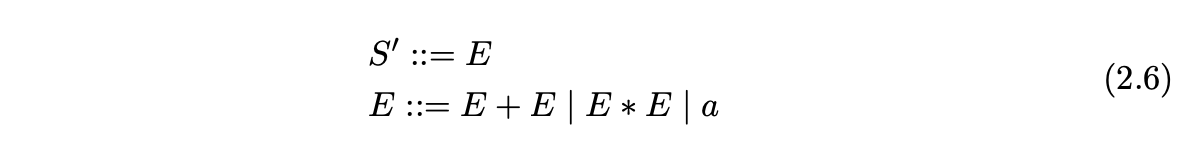
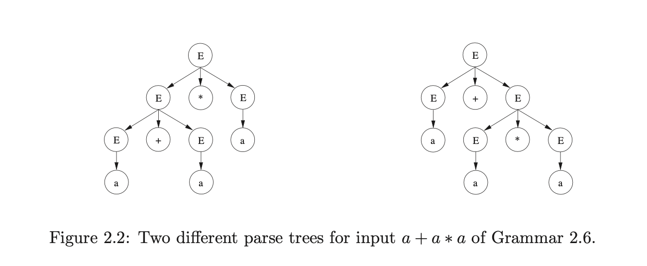
For some grammars it turns out that certain strings have more than one parse tree. These grammars are called ambiguous. For example, consider Grammar 2.6, which defines the syntax of simple arithmetic expressions.

There are two parse trees that can be constructed for the string $a+a*a$ which are shown in Figure 2.2. Clearly the searching involved in parsing ambiguous grammars can be expensive. Since context-free grammars are used to define the syntax of programming languages their parsers play an important role in the compilation process of a program, and thus need to be as efficient as possible. As a result several techniques have been developed that are capable of parsing certain non-ambiguous grammars efficiently. The next section focuses on a class of grammars for which an efficient bottom-up parsing technique can be mechanically produced.

2.4 Parsing deterministic context-free grammars¶

A computer can be thought of as a finite state system and theoreticians often describe what a computer is capable of doing using a Turing machine as a model. Turing machines are the most powerful type of automaton, but the construction and implementation of a particular Turing machine is often infeasible. Other types of automata exist that are useful models for many software and hardware problems. It turns out that the deterministic pushdown automata (DPDA) are capable of modeling a large and useful subset of the context-free grammars. Although these parsers do not work for all context-free grammars, the syntax of most programming languages can be defined by them.

In his seminal paper [10] Donald Knuth presented the LR parsing algorithm as a technique which could parse the class of deterministic context-free grammars in linear time. This section presents that algorithm and shows how the required automata are constructed.

2.4.1 Constructing a handle finding automaton¶

One of the fundamental problems of any shift-reduce parser is the location of the handle in a sentential form. The approach taken in the previous section compared each sentential form with all the production rules until a handle was found. Clearly this approach is far from ideal.

It turns out that it is possible to construct a Non-deterministic Finite Automaton (NFA) from a context-free grammar to recognise exactly the handles of all possible sentential forms. A finite automaton is a machine that uses a transition function to move through a set of states given a string of symbols. One state is defined to be the automaton’s start state and at least one state is defined as an accept state.

We now give a brief description of an NFA for a grammar. Full details can be found in texts such as [ASU86]. Our description here is based on that given in [GJ90].

Finite automata are often represented as transition diagrams, where the states are depicted as nodes and the transition function is defined by the labelled edges between the states. We can construct a finite automaton that accepts the handles of a context-free grammar by labeling the edges with grammar symbols and using the states to represent the substring of a production rule that has been recognised in a derivation. Each of the states are labelled by an item - a production rule of the form ($A::=\alpha\cdot\beta$) where the substring to the left of the $\cdot$ symbol is a viable prefix of a handle. The accept states of the automaton are labelled by an item of the form ($A::=\alpha\beta\cdot$) which indicates that the handle $\alpha\beta$ has been located.

We build the NFA of a context-free grammar by first constructing separate NFA’s for each of the grammar’s production rules. Given a rule $A::=\alpha\beta$ we create the start state of the automaton labelled by the item ($A::=\cdot\alpha\beta$). For each state that is labelled by an item of the form ($A::=\alpha\cdot x\beta$), we create a new state labelled ($A::=\alpha x\cdot\beta$) and add an edge, labelled $x$, between the two states.

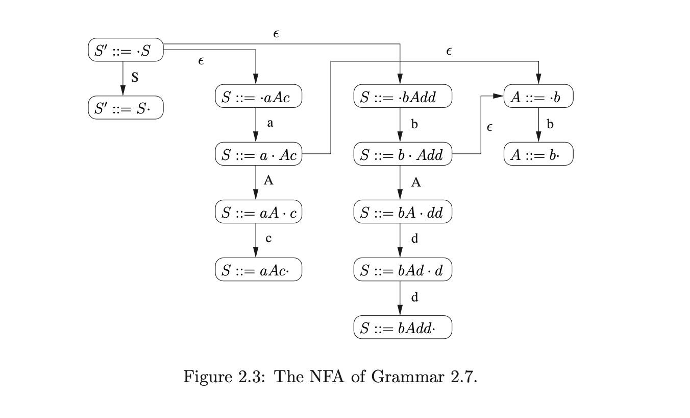
These separate automata recognise all right hand sides of a grammar’s production rules. Although this includes the handles of any sentential form, they also recognise the substrings that are not handles. We can ensure that only handles are recognised by only considering the right hand sides of rules that can be derived from the start rule of the grammar. To achieve this, the automata are joined by $\epsilon$ transitions from the states that are labelled with items of the form ($A::=\alpha\cdot B\beta$), to the start state of the automaton for $B$’s production rule. The start state of this new combined automaton is the state labelled by the item ($S^{\prime}::=\cdot S$). 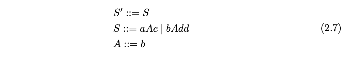For example, the NFA for Grammar 2.7 is shown in Figure 2.3.

To recognise a handle of a sentential form we traverse a path from the start state of the NFA labelled by the symbols in the sentential form. If we end up in an accept state, then we have found the left-most handle of the sentential form.

The traversal is complicated by the fact that the automaton is non-deterministic. For now we take the straightforward approach and follow all traversals in a breadth-first manner. For example, consider the sentential form $abc$ and the NFA in Figure 2.3. We begin by traversing the two $\epsilon$-edges from the start state. The states we reach are labelled ($S::=\cdot aAc$) and ($S::=\cdot bAdd$). We read the first symbol in the sentential form and traverse the edge to state ($S::=a\cdot Ac$). Because we cannot traverse the edge labelled $b$ from state ($S::=\cdot bAdd$) we abandon that traversal.

From the current state there is one edge labelled $A$ and another labelled $\epsilon$. Since the next symbol is not $A$ we can only traverse the $\epsilon$-edge that leads to the state labelled ($A::=\cdot b$). From there we read the $b$ and traverse the edge to state ($A::=b\cdot$). Since this state is an accept state, we have successfully found the handle $A$ in the sentential form $abc$.

Although this approach to finding handles can be used by bottom-up parsers, the non-deterministic nature of the NFA makes the traversal inefficient. However, it turns out that it is possible to convert any NFA to a Deterministic Finite Automaton (DFA) with the use of the subset construction algorithm [AU73].

The subset construction algorithm performs the $\epsilon$-closure from a node, $v$, to find the set of nodes, $W$, that can be reached along a path of $\epsilon$-edges in the NFA. A new node, $y$ is constructed in the DFA that is labelled by the items of the nodes in $W$. Then for the set of nodes, $\gamma$, that can be reached by an edge labelled $x$ from a node in $W$, we create a new node $z$ in the DFA. We label $z$ with the items of the nodes in $\gamma$ and the items of the nodes found by performing the $\epsilon$-closure on each node in $\gamma$. We begin the subset construction from the start state of the NFA and continue until no new DFA nodes can be created.

The node created by the $\epsilon$-closure on the start state of the NFA becomes the start state of the DFA. The accept states of the DFA are labelled by items of the form $A::=\beta\cdot$. Performing the subset construction on the NFA in Figure 2.3, we construct the DFA in Figure 2.4.

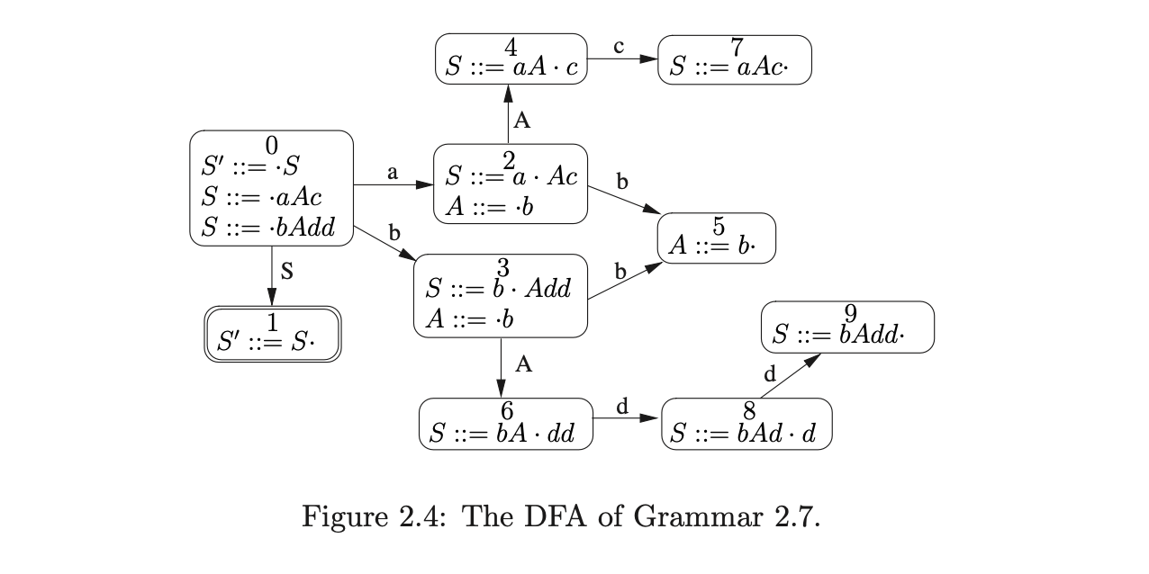A DFA is an NFA which has at most one transition from each state for each symbol and no transitions labelled $\epsilon$. It is customary to label each of the states of a DFA with a distinct state number which can then be used to uniquely identify the states. We shall always number the start state of a DFA $0$. The state labelled by the item $S^{\prime}::=S\cdot$ is the final accepting state of the DFA and is drawn with a double circle.

Parse tables

It is often convenient to represent a DFA as a table where the rows are labelled by the DFA’s state numbers and the columns by the symbols used to label the transitions between states. In addition to the terminal and non-terminal symbols that label the transitions of the DFA, the LR parse tables also have a column for the special end-of-string symbol $\$$.

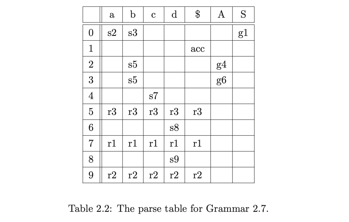
So as to avoid including the rules used by a reduction in the parse table, we enumerate all of the alternates in the grammar with distinct integers. For example, we label the alternates in Grammar 2.7 in the following way.

The parse table for Grammar 2.7 is constructed from its associated DFA in the following way. For each of the transitions labelled by a terminal, $x$, from a state $v$ to a state $w$, a shift action, s$w$ is added to row $v$, column $x$. If $x$ is a non-terminal then a goto action, g$w$, is added to entry $(v,x)$ instead. For each state $v$ that contains an item of the form $(A::=\beta\cdot)$, where $N$ is the item’s associated rule number, r$N$ is added to all entries of row $v$ whose columns are labelled by terminals and $\$$. The accept action acc is added to the row labelled by the accept state of the DFA and column $\$$. The parse table for Grammar 2.7 is shown in Figure 2.2.

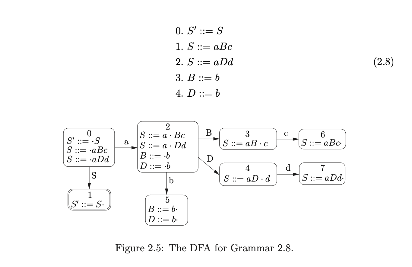
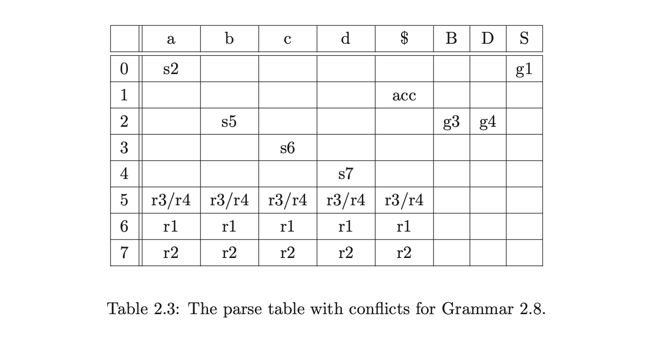
Certain grammars generate parse tables with more than one action in a single entry. Such entries are called conflicts. There are two types of conflict that can occur: the first, referred to as a shift/reduce conflict, contains one shift and one or more reduce actions in an entry; the second, called a reduce/reduce conflict, has more than one reduce action in a single state. For example, consider Grammar 2.8 and the DFA shown in Figure 2.5. The associated parse table in Table 2.3 has a reduce/reduce conflict in state 5.

2.4.2 Parsing with a DFA¶

We have seen that a DFA can be constructed from an NFA that accepts precisely all handles of a sentential form. It is straightforward to perform a deterministic traversal of this DFA to find a handle of a sentential form. In fact, we extend this traversal to determine if a string is in the language of the associated grammar.

We begin by reading the input string one symbol at a time and performing a traversal through the DFA from its start state. If an accept state is reached for the input consumed, then the leftmost handle of the current sentential form has been located. At this point the parser replaces the string of symbols in the sentential

form that match the right hand side of the handle’s production rule, with the non-terminal on the left hand side of the production rule. Parsing then resumes with the new sentential form from the start state of the DFA. If an accept state is reached and the start symbol is the only symbol in the sentential form, then the original string is accepted by the parser.

The approach of repeatedly feeding the input string into the DFA is clearly inefficient. The initial portion of the input may be read several times before its handle is found. Consequently a stack is used to record the states reached during a traversal of a given string. When an accept state is reached and a handle $\gamma$ has been located, the top $|\gamma|$ states are popped off the stack and parsing resumes from the new state at the top of the stack. This prevents the initial portion of the input being repeatedly read.

Next we discuss the LR parsing algorithm that uses a stack to perform a traversal of a DFA.

2.4.3 LR parsing¶

Knuth’s LR parser parses all LR grammars in at most linear time. An LR grammar is defined to be a context-free grammar for which a parse table without any conflicts can be constructed. Strictly speaking there are different forms of LR DFA, LR(0), SLR(1), LALR(1) and LR(1). For the moment we shall not specify which form we are using, the following discussion applies to all of them.

An LR parser works by reading the input string one symbol at a time until it has located the leftmost handle $\gamma$ of the input. At this point it reduces the handle by popping $|\gamma|$ states off the stack and then pushing the goto state onto the stack. A parse is successful if all the input is consumed and the state on the top of the stack is the DFA’s accept state. The formal specification of the algorithm is as follows.

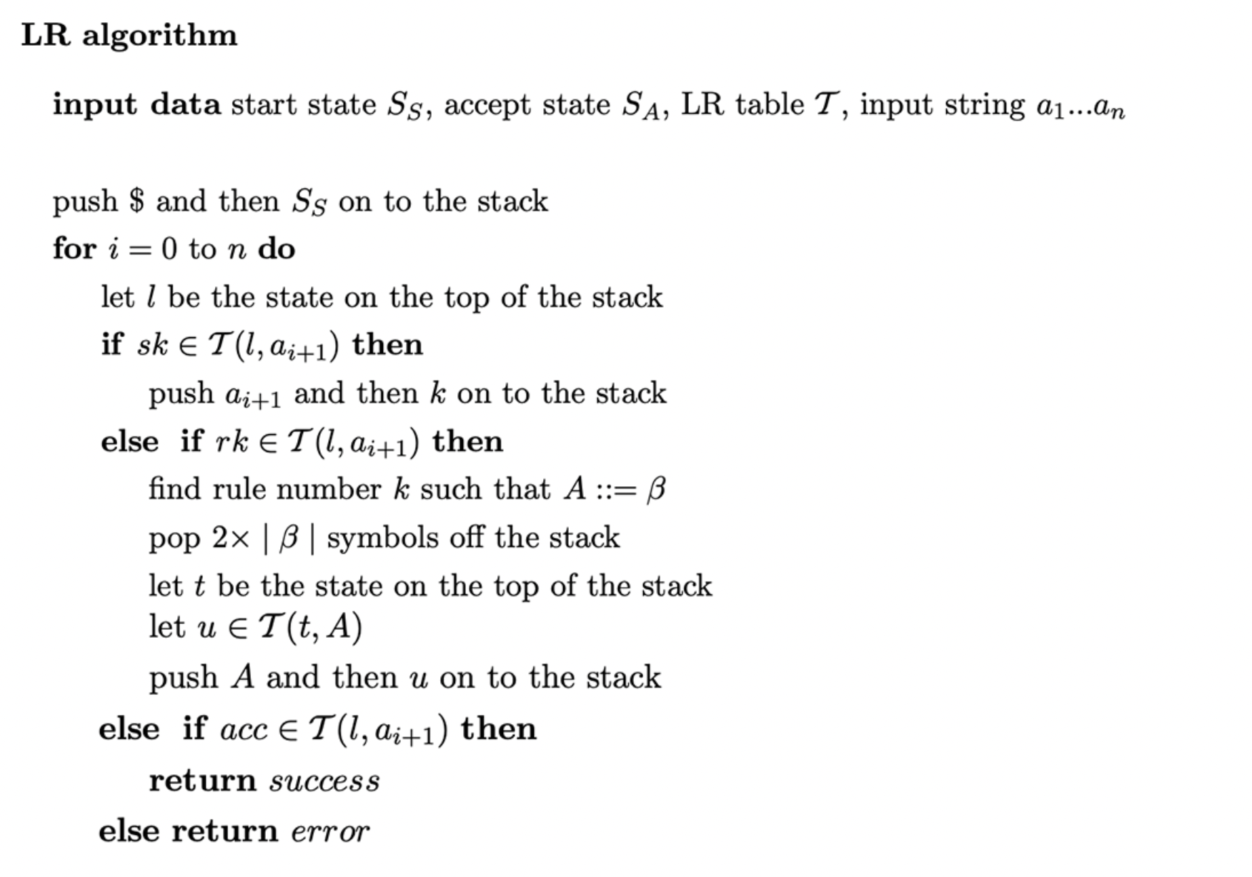
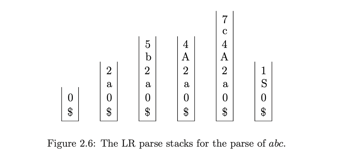
To demonstrate the operation of the LR parsing algorithm we trace the stack activity during the parse of the string $abc$ with Grammar 2.7 and the parse table shown in Table 2.2. Figure 2.6 shows the contents of the stack after every action is performed in the parse.

Although it is not strictly necessary to push the recognised symbols onto the stack, we do so here for clarity. However, it is now necessary to pop twice as many elements as the rule’s right hand side when a reduction is performed. In order to know when all the input has been consumed the special end-of-string symbol, $\$$, is added to the end of the input string.

We begin the parse by pushing $\$$ and the start state of the DFA onto the stack. Since no reduction is possible from state $0$, we read the first input symbol, $a$, and perform the shift to state $2$ by pushing the $a$ and then $2$ onto the stack. From state $2$ we read the next symbol, $b$, and perform the shift to state $5$. State $5$ contains a reduction by rule $3$, $A::=b$, so we pop the top two symbols off the stack to reveal state $2$. The parse table contains the goto $g4$ in entry $(2,A)$, so we push $A$ and then $4$ onto the stack. We continue by pushing the next input symbol, $c$, and state $7$ onto the stack for the action $s7$ in state $4$. The reduce by rule $1$, $S::=aAc$, causes the top $6$ elements to be popped and $S$ and the goto state $1$ to pushed onto the stack. Since the next input symbol is $\$$ and the parse table contains the $acc$ action in entry $(1,\$)$, the string $abc$ is accepted by the parser.

2.4.2 Parsing with lookahead¶

The DFA we have described up to now is called the LR(0) DFA. The LR parsing algorithm requires the parse table to be conflict free, but it is very easy to write a grammar which is not accepted by an LR(0) parser. The problem arises when there is a conflict (more than one action) in a parse table entry. For example, consider Grammar 2.8 and the associated parse table shown in Table 2.3.

It turns out that for some grammars these types of conflicts can be resolved with the addition of lookahead symbols to items in the DFA. For the above example, the reduce/reduce conflict can be resolved with the use of just one symbol of lookahead to guide the parse. In the remainder of this section we discuss ways to utilise a single symbol of lookahead.

For a non-terminal $A$ we define a lookahead set to be any set of terminals which immediately follow an instance of $A$ in the grammar. A reduction ($A::=\alpha\cdot$) is only applicable if the next input symbol, the lookahead, appears in the given lookahead set of $A$. In order to define useful lookahead sets we require the following definitions.

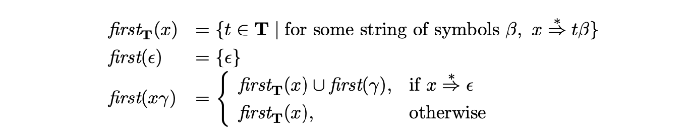
For a non-terminal $A$ we define If there is a derivation of the form $S\stackrel{{*}}{{\Rightarrow}}\beta A$ then $\$$ is also added to $\mbox{\it follow}(A)$. In particular, $\$\;$$\in\mbox{\it follow}(S)$[SJ04].

We now consider two types of LR DFA, SLR(1) and LR(1), that differ only in the lookahead sets that are calculated.

SLR(1)¶

We call a lookahead set of a non-terminal $A$global when it contains all terminals that immediately follow some instance of $A$. This is precisely the largest possible lookahead set for $A$ and is exactly the set $\mbox{\it follow}(A)$. The SLR(1) DFA construction uses these global lookahead sets. A reduction is in row $h$ and column $x$ of the SLR(1) parse table if and only if ($A::=\alpha\cdot$) is in $h$ and $x\in\mbox{\it follow}(A)$.

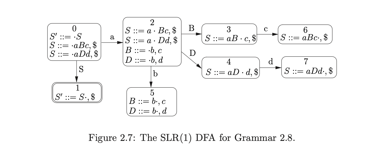
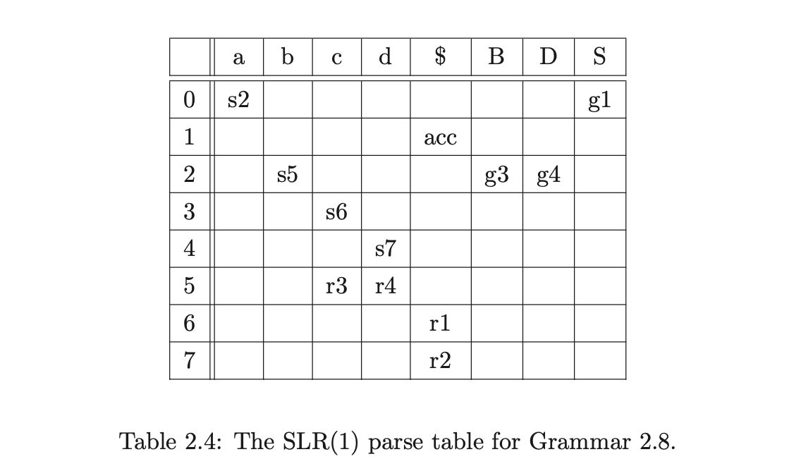
Consider Grammar 2.8. The LR(0) parse table shown in Table 2.5 contains a reduce/reduce conflict in state 5. If instead we construct the SLR(1) DFA the corresponding parse table has no conflicts as can be seen in Figure 2.7 and Table 2.4.

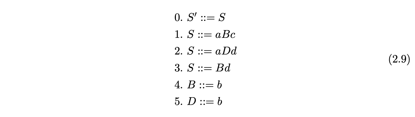
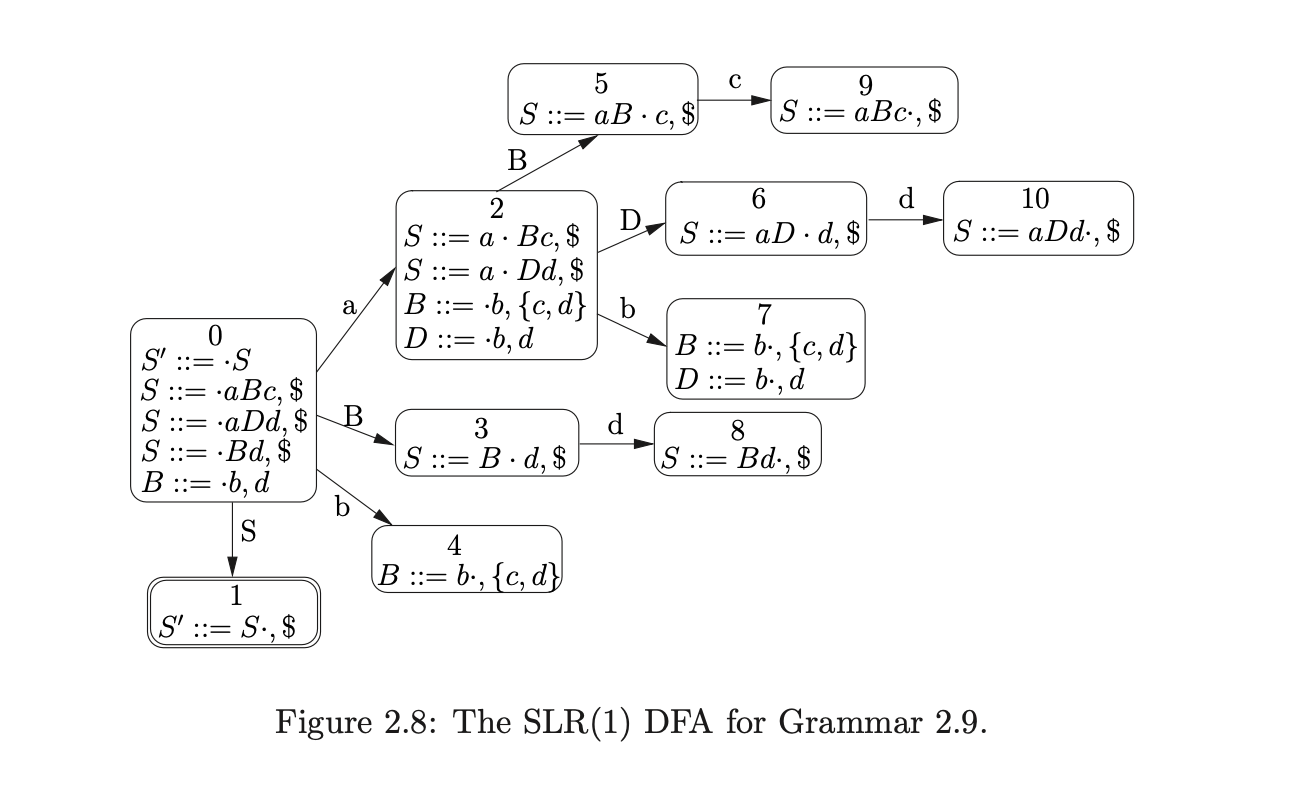
However, it is easy to come up with a grammar that does not have an SLR(1) parse table. For example consider Grammar 2.9. The associated SLR(1) DFA contains a reduce/reduce conflict in state 7.

LR(1)

Instead of calculating the global lookahead set we can further restrict the applicable reductions by calculating a more restricted lookahead set. We call a lookahead set local when it contains the terminals that can immediately follow a particular instance of a non-terminal.

In the LR(1) DFA construction local lookahead sets are used in the following way. For a state containing an item of the form $(B::=\alpha\cdot A\beta,\gamma)$ the subsequent reduction for a rule defined by $A$ contains the local lookahead set for this instance of $A$ calculated by $\mathit{first}(\beta\gamma)$.

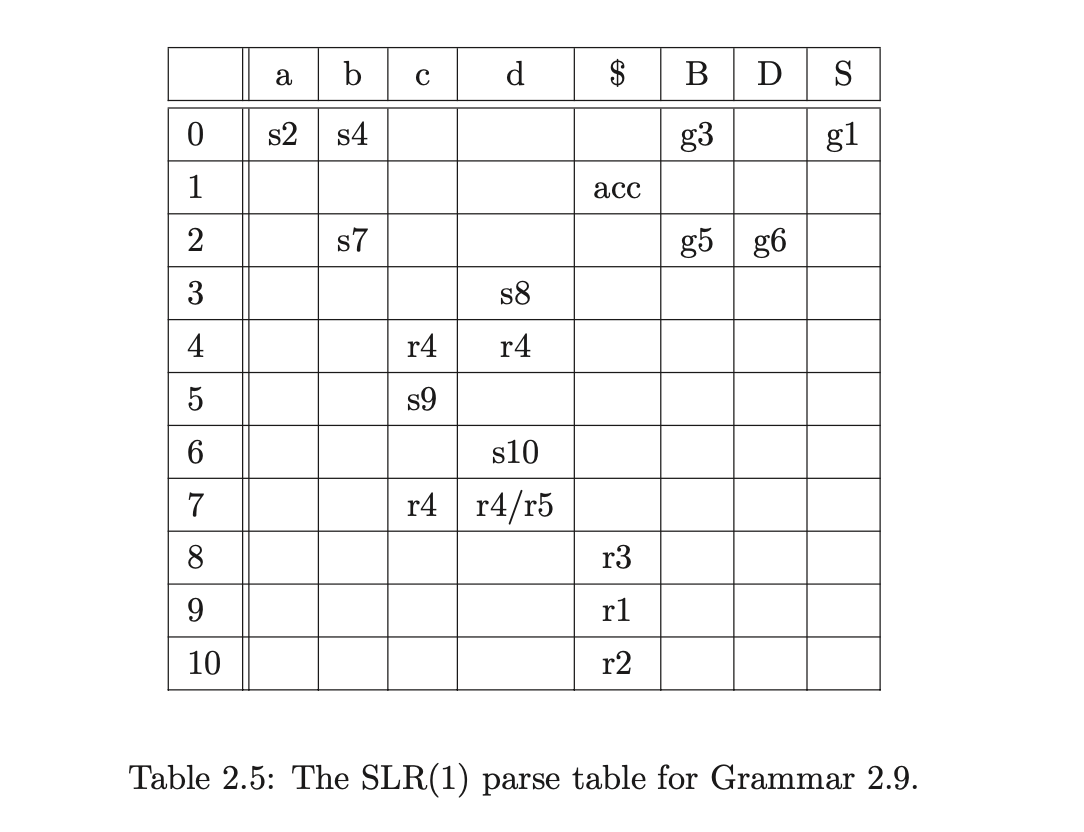
For example, the LR(1) DFA of Grammar 2.9 eliminates the reduce/reduce conflict in state 7 of Figure 2.8 and Table 2.5 by restricting the lookahead set of the reduction $(B::=b\cdot)$ from $\{c,d\}$ to $\{c\}$. This is because the item originates from $(S::=a\cdot Bc,\$)$ in state 2. The local lookahead set for the instance of $B$ in $S::=aBc$ is $\{c\}$. (See [1] for full details on LR(1) DFA construction.)

The set of LR(1) grammars strictly includes the SLR(1) grammars. However, in many cases this extra power comes at the price of a potentially large increase in the number of states in the DFA. We discuss the size of the different parse tables in Chapter 10.

The LR(1) DFA construction was defined in Knuth’s seminal paper on LR parsing [10], but at the time the LR(1) parse tables were too large to be practical. DeRemer later developed the SLR(1) and LALR(1) DFA’s in order to allow more sharing of nodes therefore reducing the size of the DFA [12].

LALR(1)

LALR(1) DFA’s are constructed by merging states in the LR(1) DFA whose items only differ by the lookahead set. The LALR(1) DFA for a grammar $\Gamma$ contains the same number of states but fewer conflicts than the SLR(1) DFA for $\Gamma$.

Using $k$ symbols of lookahead

Although it is possible to increase the amount of lookahead that a parser uses, it is not clear that the extra work involved is justified. The automata increase in size very quickly, and for every LR(k) parser it is easy to write a grammar which requires $k+1$ amount of lookahead.

2.5 Summary¶

This chapter has presented the theory and techniques that are needed to build an LR parser. LR parsers are the most powerful deterministic parsing technique, but despite being used to define the syntax of many modern programming languages, it is easy to write a grammar which is not LR(1). The next chapter paints a picture of the landscape of some of the important generalised parsing techniques (that can be applied to all context-free grammars) developed over the last 40 years.