6.Binary Right Nulled Generalised LR parsing¶

Despite the fact that general context-free parsing is a mature field in Computer Science, its worst case complexity is still unknown. The algorithm with the best asymptotic time complexity to date is presented in [25] by Valiant. His approach uses Boolean matrix multiplication (BMM) to construct a recognition matrix that displays the complexity of the associated BMM algorithm. Since publication of Valiant’s paper, more efficient BMM algorithms have been developed. The algorithm with currently the lowest asymptotic complexity displays $O(n^{2.376})$ for $n\times n$ matrices [13, 14].

Although the approach taken by Valiant is unlikely to be used in practice, because of the high constant overheads, it was an important step toward understanding more about the complexity of general context-free parsers. A related result has been presented by Lee which maps a context-free parser with $O(n^{3-\epsilon})$ complexity to an algorithm to multiply two $n\times n$ Boolean matrices in $O(n^{3-(\epsilon/3)})$ time. A side effect of this work has led to the hypothesis that ‘practical parsers running in significantly lower than cubic time are unlikely to exist’ [16]. Although this analysis does suggest that linear time parsers are unlikely to exist, it does not preclude quadratic algorithms from being developed.

Two other general parsing algorithms that have been used in practice are the CYK and Earley algorithms. Both display cubic worst case complexity, although the CYK algorithm requires grammars to be transformed to CNF before parsing. Unfortunately this complexity is still too high for certain applications; most programming languages have largely deterministic grammars which can be parsed by linear parsers. The GLR algorithm first developed by Tomita, provides a general parsing algorithm that takes advantage of the efficiency of the deterministic LR parsers. Unfortunately these algorithms display unbounded polynomial time and space complexity [15].

This chapter presents an algorithm which is based on the RNGLR algorithmdescribed in Chapter 5, but which has a worst case complexity of $O(n^{3})$ without requiring any transformations to be done to the grammar.

6.1 The worst case complexity of GLR recognisers¶

In Chapter 2 we examined the operation of a standard bottom-up shift reduce parser. Recall that such a parser works by using a stack to collect symbols of a sentential form and then when it recognises a handle, of length $m$ say, it pops the $m$ symbols off the stack and pushes on the left hand non-terminal of the corresponding rule. An important feature of such shift reduce parsers is that it is not necessary to examine the symbols on the stack before they are popped. The associated automaton guarantees that when a reduction for a rule $A::=\beta$ is performed, the top $m$ symbols on the stack are equal to $\beta$. Implementations of such parsers exploit this property and perform reductions in unit time by simply decrementing the stack pointer. In comparison, general parsing algorithms that extend such parsers cannot perform reductions as efficiently.

It is well known that the worst case time complexity of Tomita’s GLR parser is $O(n^{M+1})$, where $n$ is the length of the input string and $M$ is the length of the longest grammar rule [15]. Although it is not entirely surprising, it is somewhat disappointing that the recogniser displays the same complexity, especially since both the Earley and CYK recognisers are cubic in the worst case. In this section we shall explain why the RNGLR recogniser is worse than cubic.

Roughly, when a GLR parser reaches a non-deterministic point in the automaton, the stack is split and both parses are followed. If the separate stacks then have a common stack top once again, the stacks are merged. This merging of stacks bounds the size of the GSS to at most $(n+1)\times H$ nodes, where $n$ is the length of the input string and $H$ is the number of states in the automaton. However, because the different stacks are now combined into one structure a reduce action can be applied down several paths from one node. Unlike the standard shift reduce parser we are not able to simply decrement a stack pointer, we need to perform a search.

It is possible for a state in level $i$ to have edges going back to states in every other level $j$, where $0\leq j\leq i$. Since a node in the GSS can have $H\times(i+1)$ edges, $i^{m}$ paths may need to be explored for any reduction of length $m+1$ that is performed. This results in such algorithms displaying $O(n^{m+1})$ time complexity. Although we will not prove this here, we shall describe a grammar and an example string that illustrate the properties which trigger quartic behaviour in the RNGLR algorithm. Clearly this is sufficient to show that the RNGLR algorithm is not cubic.

Example - Recognition in $O(n^{4})$ time¶

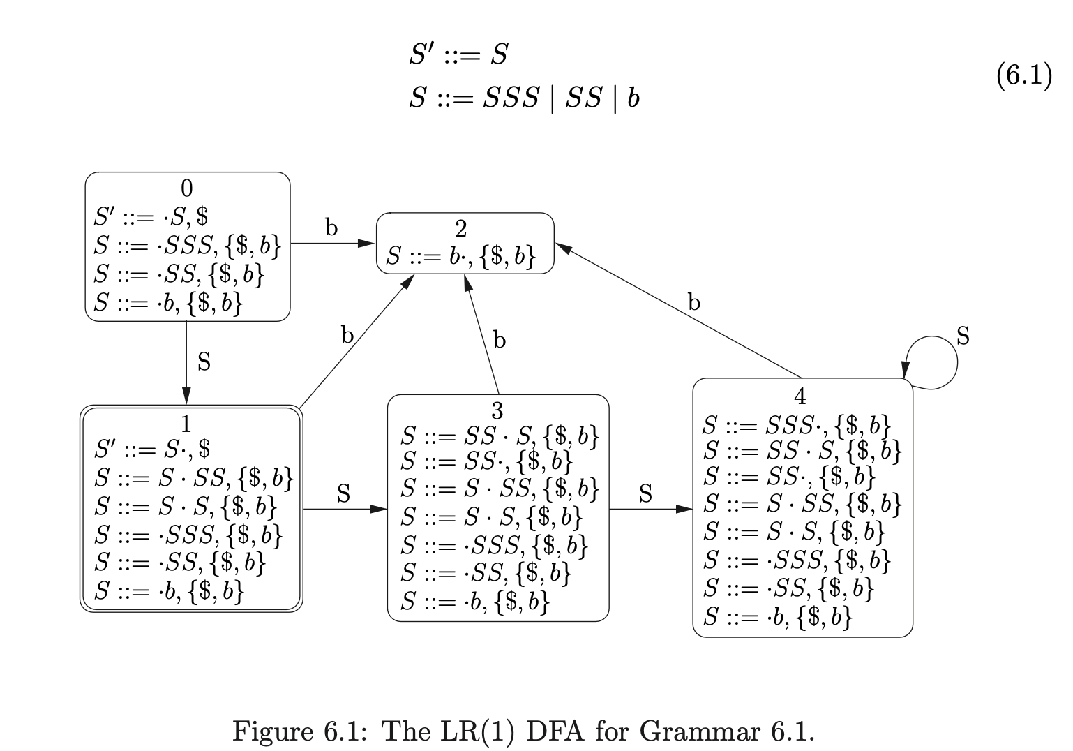
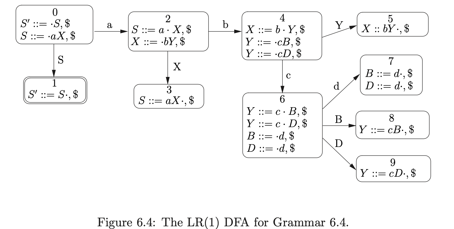
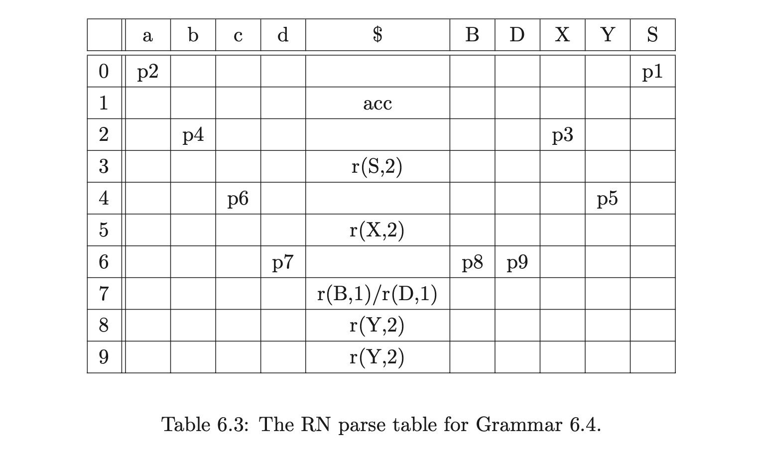
Consider Grammar 6.1, its LR(1) DFA in Figure 6.1 and the associated RN parse table $\mathcal{T}$ in Table 6.1.

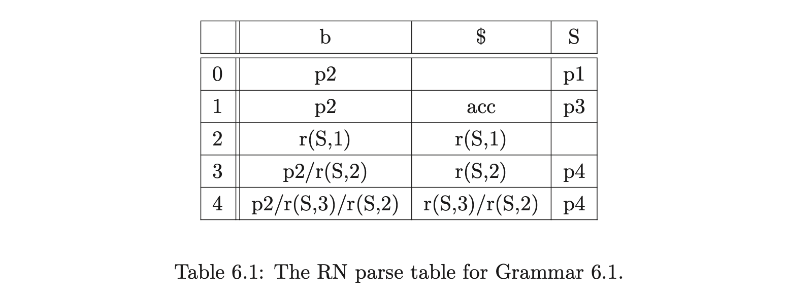
We can illustrate the properties that cause the RNGLR algorithm to have at least $O(n^{4})$ time complexity, by parsing the string $bbbbb$. We begin by creating the node $v_{0}$ labelled with the start state of the DFA. The shift action $p2$ is the only element in $\mathcal{T}(0,b)$, so we perform the shift and create the new node $v_{1}$ labelled $2$. As there is the reduce action $r(S,1)$ in $\mathcal{T}(2,b)$, $(v_{0},S,1)$ is added to the set $\mathcal{R}$. When $(v_{0},S,1)$ is removed from $\mathcal{R}$, the node $v_{2}$ labelled $1$ is created.

Processing $v_{2}$ we find that the shift $p2$ is the only action in $\mathcal{T}(0,b)$ so we create the node $v_{3}$ labelled $2$ in the next level and add $(v_{2},1)$ since $r(S,1)$ is in $\mathcal{T}(2,b)$. By performing the reduce in $\mathcal{R}$ we create node $v_{4}$ labelled $3$ and the edge from $v_{4}$ to $v_{2}$. Examining the entry in $\mathcal{T}(3,b)$ we find that there is a shift/reduce conflict with actions $p2/r(S,2)$. We add the actions to the sets $\mathcal{Q}$ and $\mathcal{R}$ respectively. Performing the reduction in $\mathcal{R}$ we create $v_{5}$ with an edge to $v_{0}$ and then add $(v_{5},S,2)$ to $\mathcal{Q}$. Once the shifts have been removed and processed from the set $\mathcal{Q}$, the new node $v_{6}$ labelled $2$ has been created in level $3$, and $(v_{4},S,1)$ and $(v_{5},S,1)$ are added to $\mathcal{R}$ because of the reduce action in $\mathcal{T}(2,b)$. When both the reductions are done the nodes $v_{7}$ and $v_{8}$, labelled $4$ and $3$ respectively, are created along with their associated edges from $v_{7}$ to $v_{4}$ and $v_{8}$ to $v_{5}$. At this point $\mathcal{R}=\{(v_{4},S,3),(v_{4},S,2),(v_{5},S,2)\}$ and $\mathcal{Q}=\{(v_{7},2),(v_{8},2)\}$. Removing $(v_{4},S,3)$ from $\mathcal{R}$, the Reducer traces back a path to $v_{0}$ and creates the new node $v_{9}$ labelled $1$, with an edge between $v_{9}$ and $v_{0}$. As $\mathcal{T}(1,b)$ contains the shift $p2$, $(v_{9},2)$ is also added to the set $\mathcal{Q}$. When $(v_{4},S,2)$ is processed the Reducer traces back a path to $v_{2}$ and creates a new edge between $v_{8}$ and $v_{2}$. As a result of the new edge, $(v_{2},S,2)$ is added to $\mathcal{R}$. When $(v_{5},S,2)$ and then $(v_{2},S,2)$ are processed, the Reducer traces back a path to $v_{0}$ once again, but since the node labelled $1$ already exists in the current level and there is an edge to $v_{0}$, nothing is done.

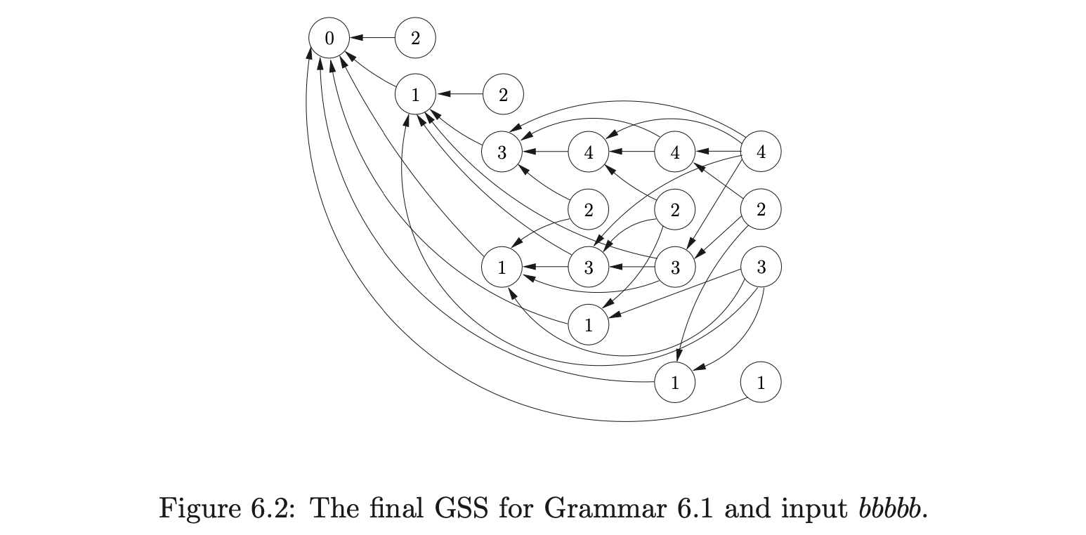
After processing the shift actions queued in $\mathcal{Q}$ the node labelled $2$ is created in level $4$, with edges going back to the nodes labelled $4$, $3$ and $1$ in the previous level.

Notice that the node labelled $4$ in the final level of the GSS in Figure 6.2 has edges that go back to every node labelled $4$ in the previous levels. This pattern is repeated when recognising any strings of the form $b^{n}$. At each level $i\geq 3$ in the GSS there is a node labelled $4$ which has edges back to the nodes labelled $3$ in each of the levels below $i$ in the GSS. It is this property that is used in [10] to prove that the RNGLR algorithm takes at least $O(n^{4})$ time when used to parse sentences $b^{n}$ using the RN parse table for Grammar 6.1. Since Tomita’s Algorithm 1e builds the same GSS as the RNGLR algorithm, they share the property that triggers this worst case behaviour.

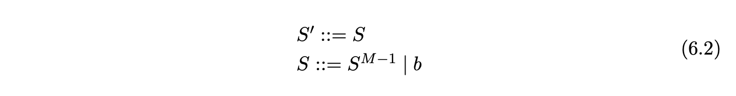
In fact the RNGLR algorithm is at most $O(n^{M+1})$, where $M$ is the longest rule in the underlying grammar for any RN parse table when $M\geq 3$. Furthermore, grammars in the form of Grammar 6.2 trigger $O(n^{M})$ behaviour in such GLR parsers.

6.2 Achieving cubic time complexity by factoring the grammar¶

The previous section discussed the properties of grammars that cause GLR recognisers to display polynomial behaviour. Since it is the searching that is done to find the target nodes of a reduction that determines the complexity of such algorithms, an obvious approach to reduce the complexity is to first reduce the searching. The length of the searches done for a reduction is directly related to the length of the grammar’s rules. Clearly, by restricting the length of the grammar’s rules, an improvement should be possible.

There are several existing algorithms that can transform any context-free grammar into another grammar whose rules have a maximum length of two [10]. One of the best known techniques, used by other parsing algorithms such as CYK, is to transform the grammar into Chomsky Normal Form (CNF). Although the algorithm that transforms a grammar to CNF produces a grammar with the desired property, it has two major drawbacks; the resulting parses are done with respect to the CNF grammar and the process to recover the derivations with respect to the original grammar can be expensive, and there is a linear increase in the size of the grammar [10].

Of course, it is not necessary to have CNF to have $O(n^{3})$ complexity. All that is required is that the grammar rules all have length at most two. We can achieve this with a grammar which is close to the original by simply factoring the rules. In this way the generated derivations can be closely related to the original grammar.

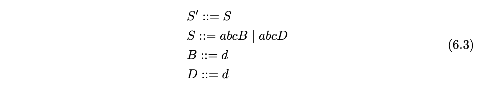
Grammar 6.4 is the result of factoring Grammar 6.3 so that no right hand side has a length greater than two. Using factored grammars the RNGLR algorithm can parse in at most cubic time.

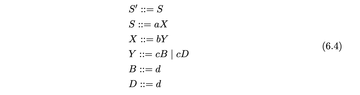
We have to be careful when introducing extra non-terminals. If we only use one non-terminal for the two alternates of $S$ in the following grammar the strings $aba$ and $cbc$ are incorrectly introduced to the language.

Thus new non-terminals need to be introduced for each reduction of each rule. Unfortunately this approach can also lead to a substantial increase in the size of the parse table. For example the $\operatorname{SLR}(1)$ parse table for our IBM-VS Cobol grammar is $2.8\times 10^{6}$ cells compared with $6.2\times 10^{6}$ for the binarised grammar. The increase is even more dramatic for some $\operatorname{LR}(1)$ tables. Our ANSI-C grammar has cells compared to the $8.0\times 10^{5}$ cells of the factorised grammar. For a more detailed discussion of parse tables sizes see Chapter 10.

6.3 Achieving cubic time complexity by modifying the parse table¶

In the previous section we showed how to use the RNGLR algorithm to achieve cubic worst case complexity by factoring the grammar before parsing. Unfortunately, this technique can dramatically increase the size of the parse table. The objective of factoring the grammar was to restrict the length of the reductions performed during parsing. In this section we present a different approach which achieves the same complexity, but does not increase the size of the parse table to the same degree.

Instead of factoring the grammar it is possible to restrict the length of reductions performed by directly modifying the parse table. This involves the creation of $N_{A}$ additional states for each non-terminal $A$, where $(N_{A}+2)$ is the longest alternate of $A$. So if $N_{A}\geq 1$ then the additional states $A_{1}\ldots A_{N_{A}}$ are created.

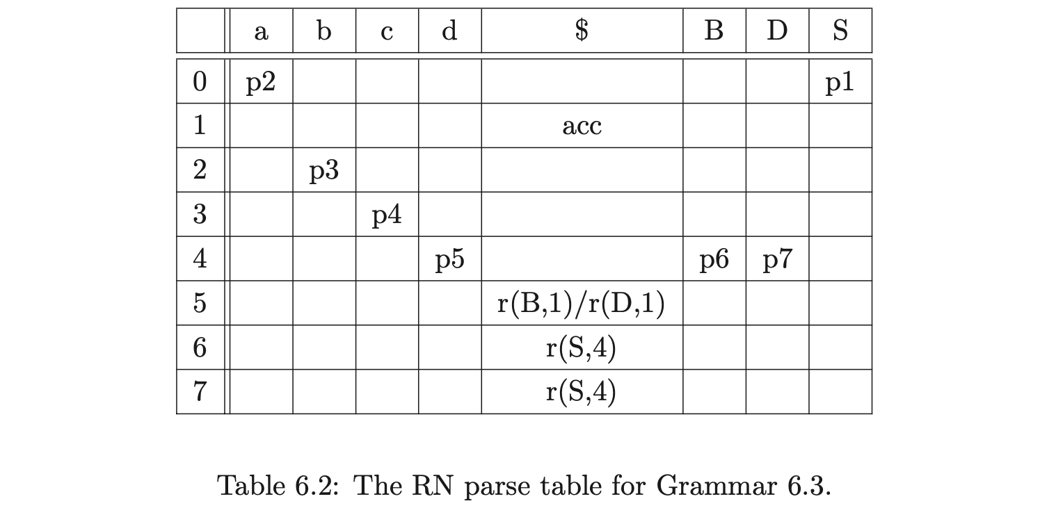
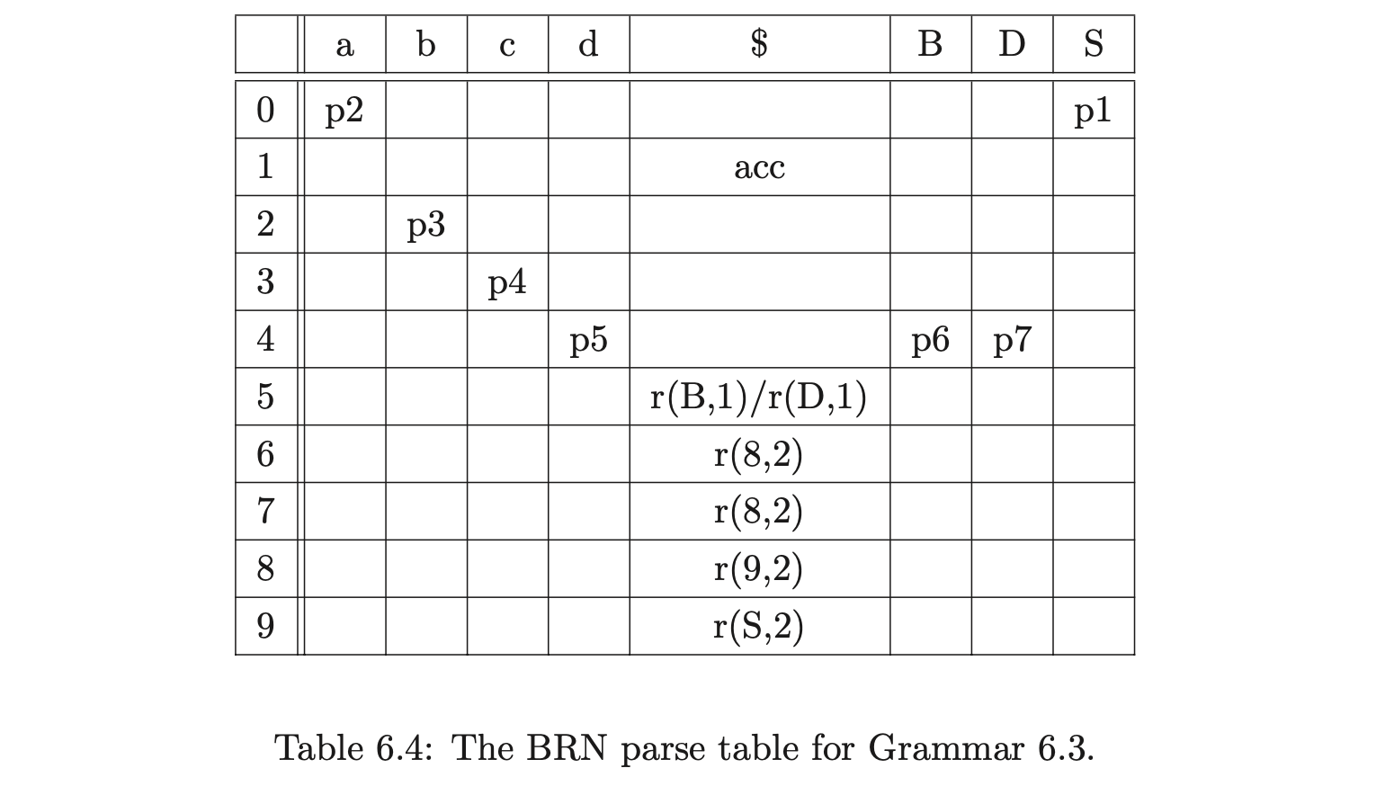
In addition to this, a new type of reduction action is added to the parse table so that only reductions with a maximum length of two are performed. The new reductions are of the form $r(A_{j},2)$, where $A_{j}$ is an additional state and $2$ is the length of the reduction. When such an action is performed two symbols are popped off the stack and $A_{j}$ is pushed onto the stack. For example consider Grammar 6.3 and the associated BRN parse table 6.4. By using the parse table shown in Table 6.4 to parse the string $abcd$, the GSS in Figure 6.5 is constructed.

Although the GSS created with the use of the BRN parse table is larger than the one created with the RN table, the increase in size is only a constant factor. Both GSS’s have $O(n^{2})$ edges, but the GSS generated by the BRN table can be constructed in at most cubic time. In [SJE03] a proof is given that shows the BRN parse table accepts exactly the same set of strings as the RN parse table. Since there is another proof in [10] that shows the RN parse table to accept precisely the same strings as an LR(1) parser for the same grammar we can be rely on the parse table being correct.

6.4 The BRNGLR recognition algorithm¶

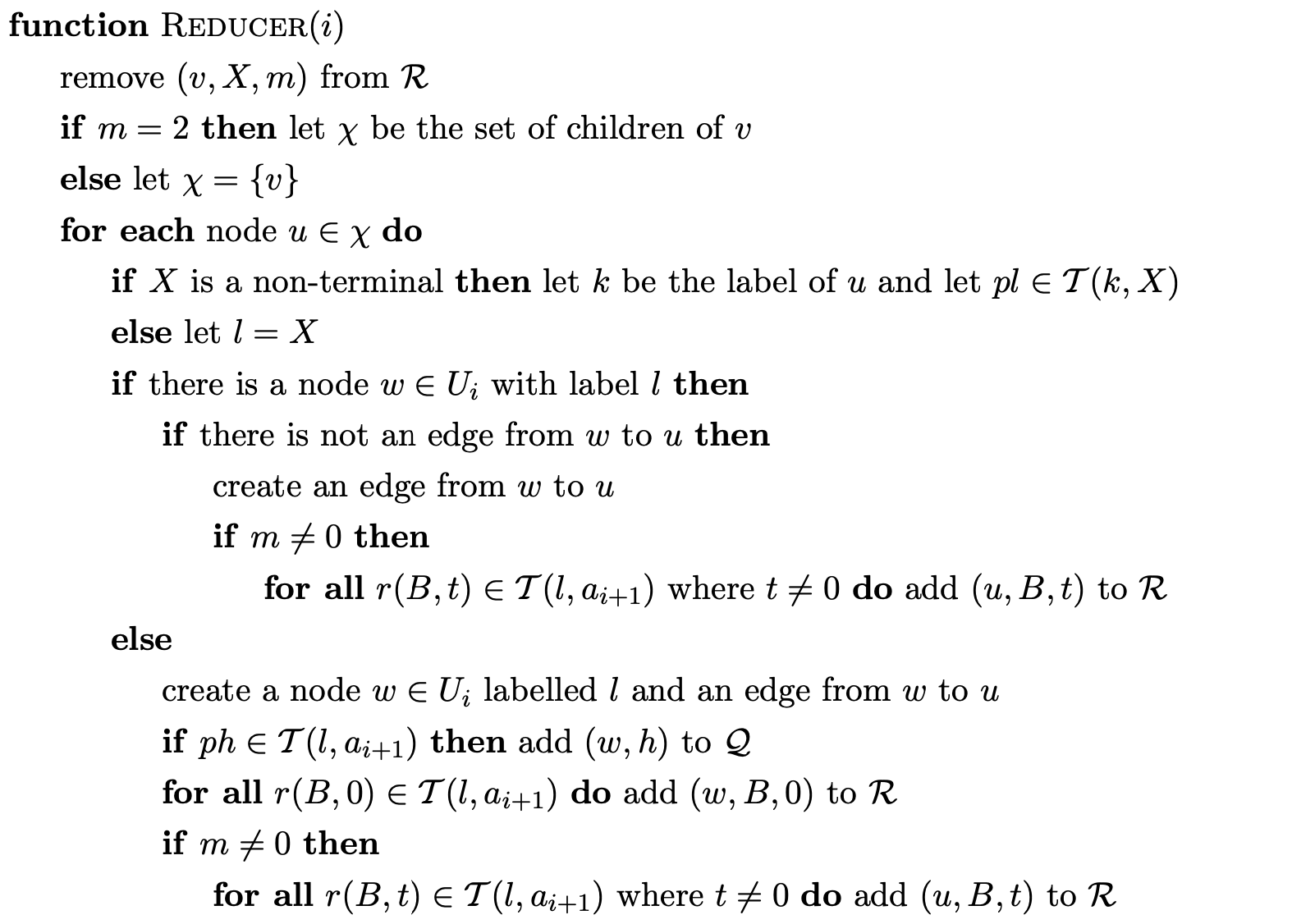
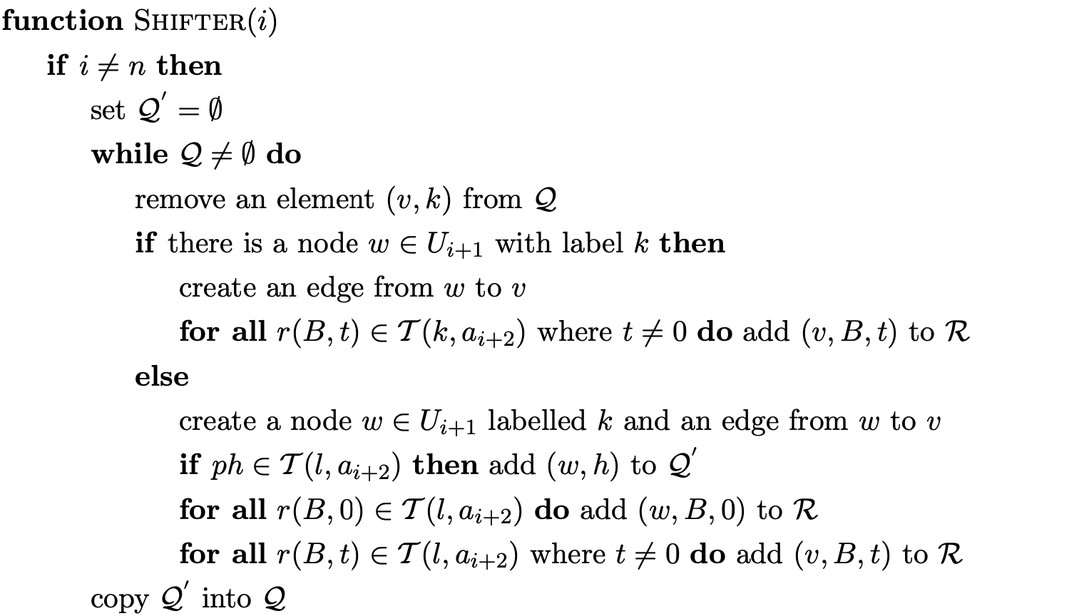
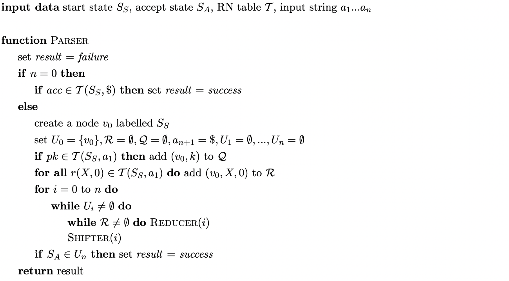
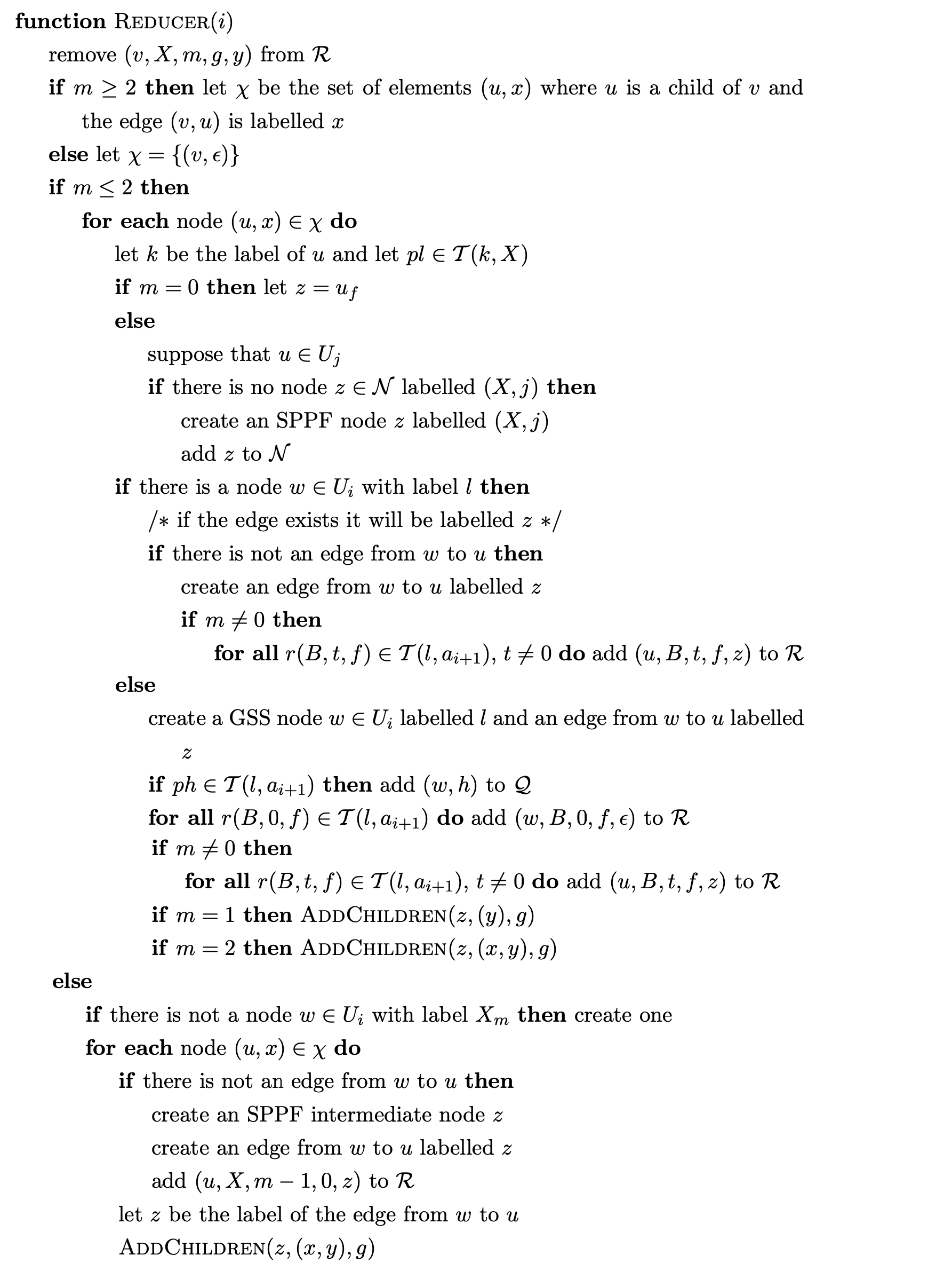
This section presents the formal definition of the BRNGLR recognition algorithm that uses BRN parse tables to parse sentences in at most cubic time.

BRNGLR recogniser¶

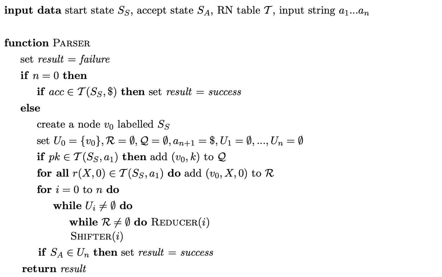
Although the above algorithm succeeds in parsing all context-free grammars in at most cubic time, it is disappointing that the parse table increases in size (eventhough the increase is only by a constant factor). It turns out that because of the regular way the additional reductions are done, it is possible to achieve the same complexity without modifying the parse table. The following section describes such an algorithm.

6.5 Performing ‘on-the-fly’ reduction path factorisation¶

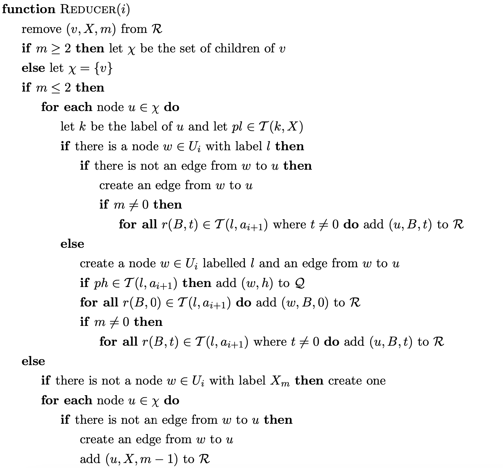
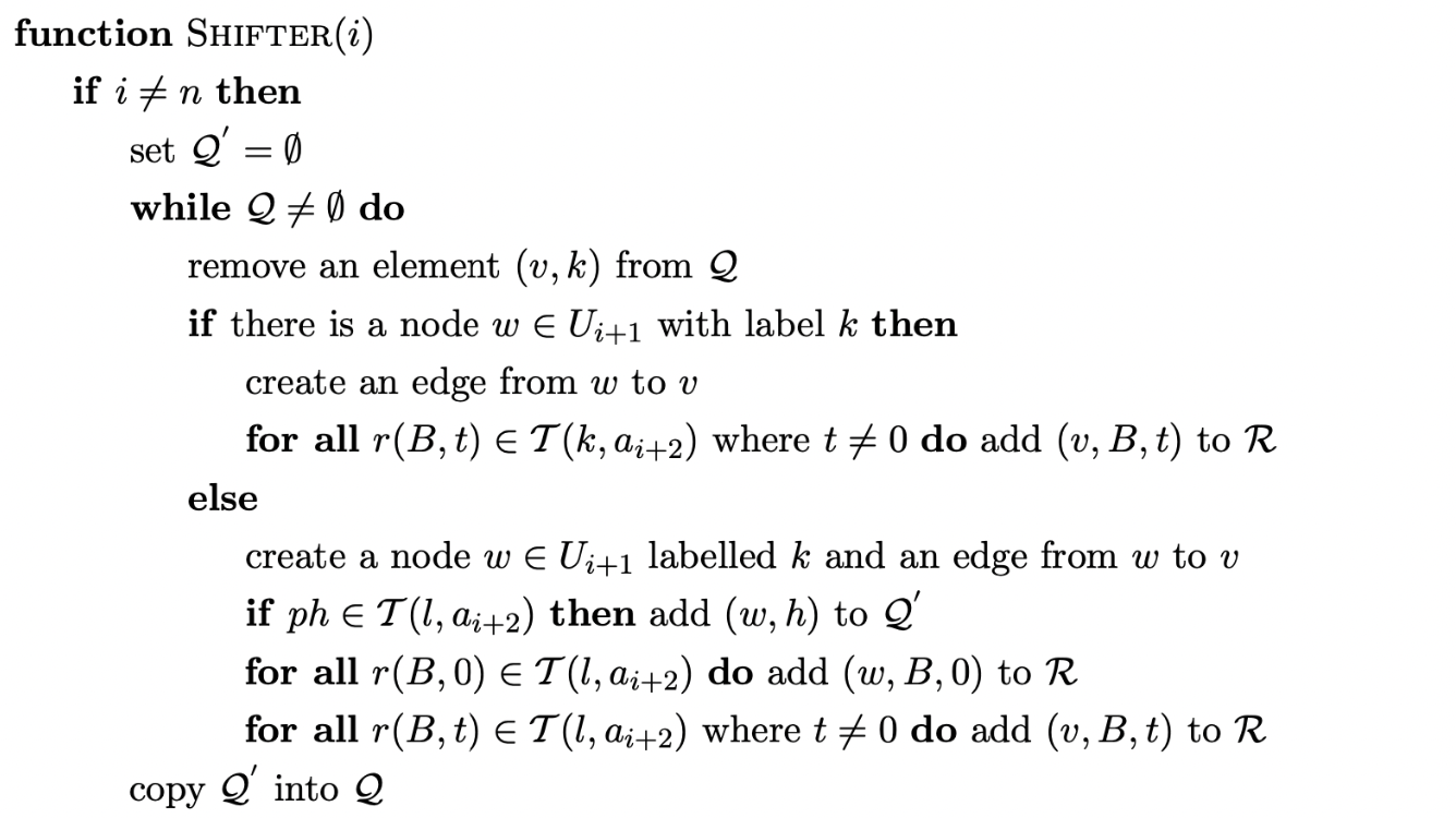
The algorithm defined in the previous section is an extension of the RNGLR algorithm which uses BRN parse tables to achieve cubic worst case time complexity. A further extension of the previous algorithm performs this binary translation ‘on-the-fly’. This algorithm works on an original RN parse table, but includes the extra machinery necessary to only carry out searches with a maximum length of two. When an action $r(X,m)$ is encountered in the parse table, the algorithm stores the pending reduction in the set $\mathcal{R}$ in the form $(v,X,m)$, where $v$ is the target of the edge down which the reduction is to be applied and $m$ is the length of the reduction. When $m>2$ a new edge is added from a special bookkeeping node labelled $X_{m}$ in the current level to every child node $u$ of $v$ and the element $(u,X,m-1)$ is added to $\mathcal{R}$. This technique ensures that reductions of length greater than 2 are done in $m-1$ steps of length two. The bookkeeping nodes prevent the repeated traversal of a path in the same way that the extra states added to the modified RN parse table do.

The on-the-fly algorithm is the preferred implementation of the BRNGLR algorithm as it does not increase the size of the RN parse table to achieve cubic worst case time complexity.

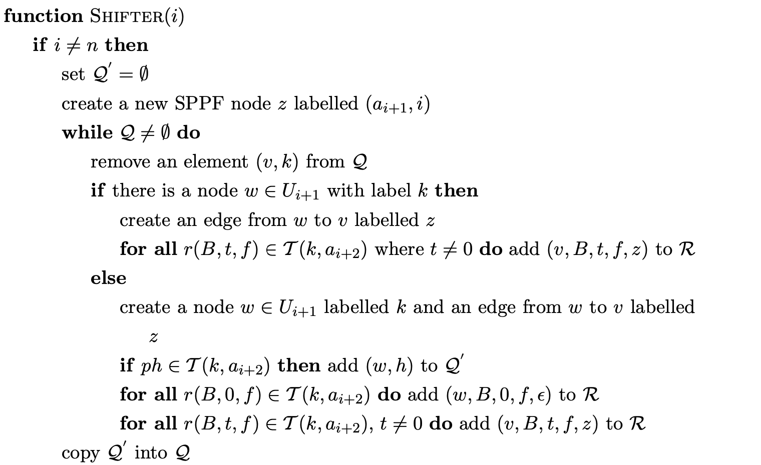
BRNGLR ‘on-the-fly’ recogniser¶

For the formal proofs on the correctness and the complexity of the BRNGLR algorithm see [SJE03].

Example - ‘on-the-fly’ recognition in $O(n^{3})$ time¶

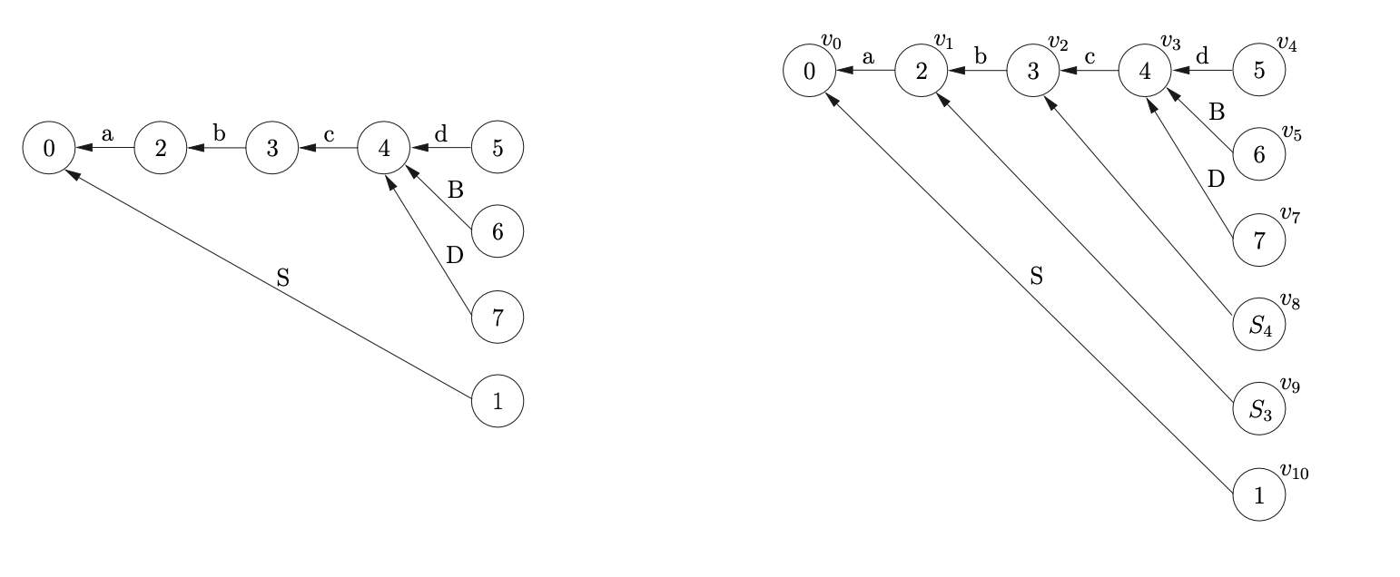
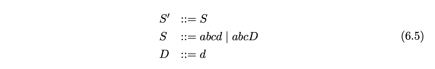
To demonstrate the operation of the ‘on-the-fly’ BRNGLR recognition algorithm we shall trace the construction of the GSS for Grammar 6.5 and the input $abcd$.

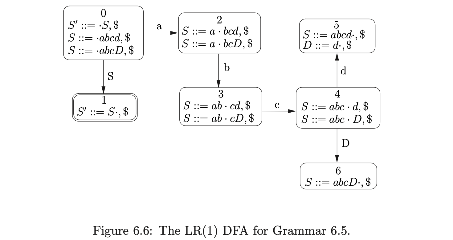
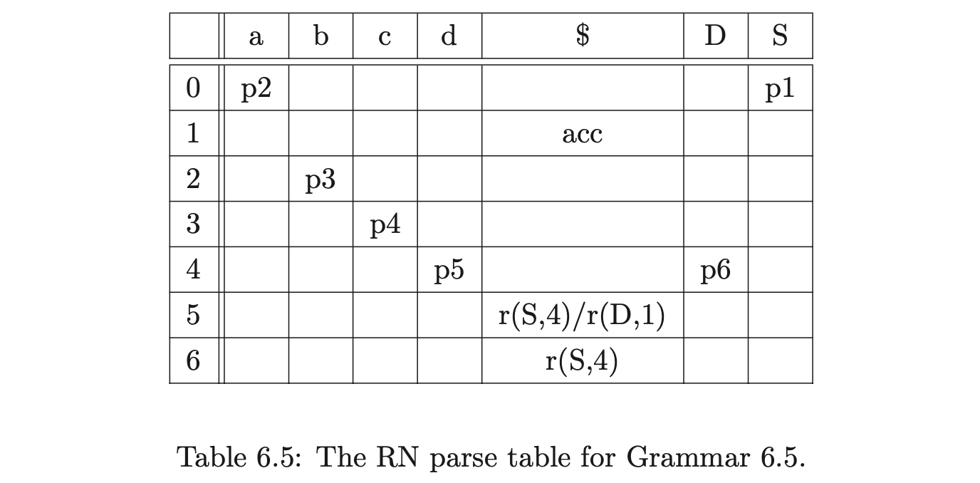As usual we begin by first creating the node $v_{0}$ labelled with the start state of the DFA in Figure 6.6 and then proceed to add the actions found in $\mathcal{T}(0,a)$ to the appropriate sets. In this case, only the shift action $p2$ is added to the set $\mathcal{Q}$, which results in the node $v_{1}$ labelled $2$ and the edge from $v_{1}$ to $v_{0}$ being created. Continuing in this way, the next three states created for the remainder of the input string result in the partial GSS shown below.

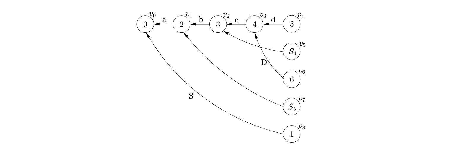
At this point we have $\mathcal{R}=\{(v_{3},S,4),(v_{3},D,1)\}$ and $\mathcal{Q}=\{\}$. When we process $(v_{3},S,4)$ we find $v_{2}$, the only child of $v_{3}$, and add it to the set $\chi$. Since there is no bookkeeping node labelled $S_{4}$ in the current level of the GSS we create one, $v_{5}$, add an edge between $v_{5}$ and $v_{3}$ and then add the additional reduction $(v_{2},S,3)$ to $\mathcal{R}$.

We then process $(v_{3},D,1)$. Since the reduction length is less than $2$, we perform a normal reduction which results in the creation of a new node, $v_{6}$, labelled $6$, with an edge back to $v_{3}$. There is a reduction $r(S,4)\in\mathcal{T}(6,\$)$ so we add $(v_{3},S,4)$ into $\mathcal{R}$.

Processing $(v_{2},S,3)$, we find $v_{1}$, the only child of $v_{2}$, and add it to $\chi$. Since there is no node labelled $S_{3}$ in the current level, we create $v_{7}$ and add an edge between $v_{7}$ and the only node in $\chi$, $v_{1}$. The final additional reduction, $(v_{1},S,2)$, is added to $\mathcal{R}$.

When we process the reduction for $(v_{3},S,4)$ we check to see if a bookkeeping node labelled $S_{4}$ already exists in the current level. It does. Because we already performed a reduction of length $4$ for a rule defined by the non-terminal $S$, whose path included $v_{3}$, we do not need to continue with the current reduction. Clearly this reduces the amount of edge visits that we perform during the parse.

We continue by performing the reduction for $(v_{1},S,2)$. We find $v_{0}$, the only child of $v_{1}$ and create the new node $v_{8}$ labelled $1$, with an edge labelled $S$ to $v_{0}$. Since we have consumed all the input and $v_{8}$ is labelled by the accept state of the DFA the input $abcd$ is successfully accepted. The final GSS is shown below.

6.6 GLR parsing in at most cubic time¶

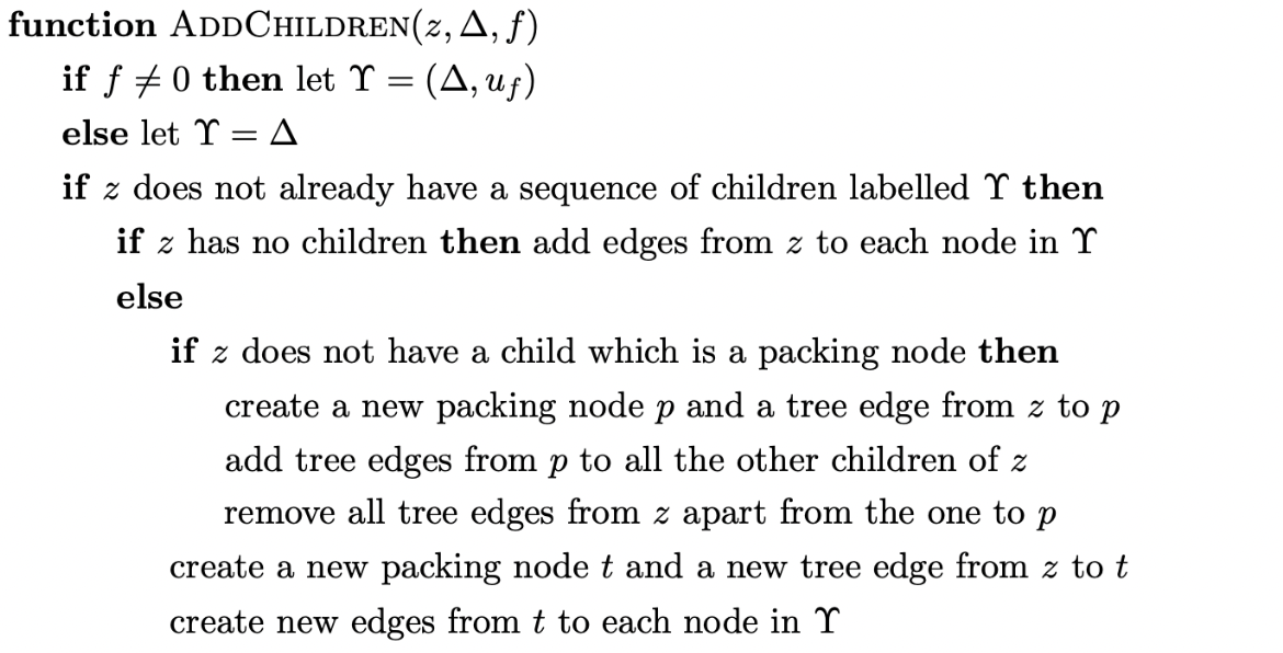
We extend the BRNGLR recognition algorithm to a parser by constructing an SPPF in a similar way to the approach we take for the RNGLR algorithm (see Chapter 5). Recall that nodes can be packed if their yields correspond to the same portion of the input string. In order to ensure that a correct SPPF is constructed care needs to be taken when dealing with the bookkeeping SPPF nodes. (Note that the bookkeeping SPPF nodes are not labelled.) We give the algorithm and then illustrate the basic issues using Grammar 6.3. We then discuss the subtleties of the use of bookkeeping nodes in Section 6.7.

BRNGLR parser¶

Layer 3.png

Example - parsing in $O(n^{3})$ time¶

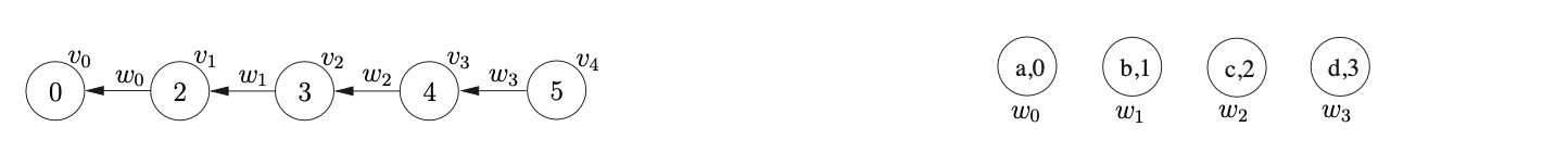
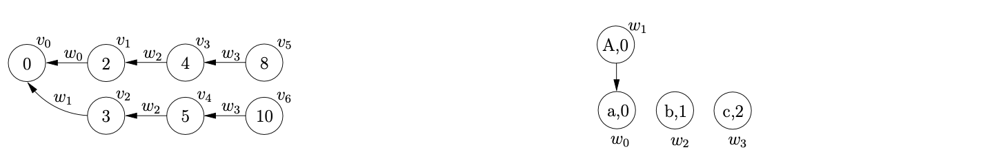
To illustrate the operation of the algorithm we shall trace the construction of the GSS and SPPF for the string $abcd$ in the language of Grammar 6.3 shown on page 6.3. We begin by constructing the GSS node $v_{0}$ labelled by the start state of the DFA. Since $p2\in\mathcal{T}(0,a)$ we create the node $v_{1}$ labelled $2$, the SPPF node $w_{0}$ labelled $(a,0)$ and the edge from $v_{1}$ to $v_{0}$ in the GSS which is labelled by $w_{0}$.

We proceed to shift the next three input symbols in the same way, which results in the GSS and SPPF shown in Figure 6.7 being constructed.

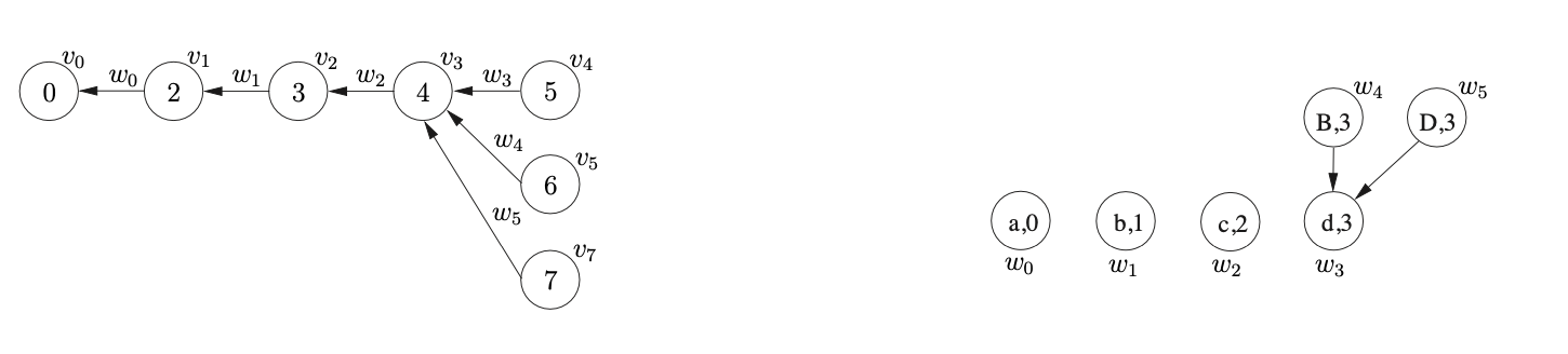
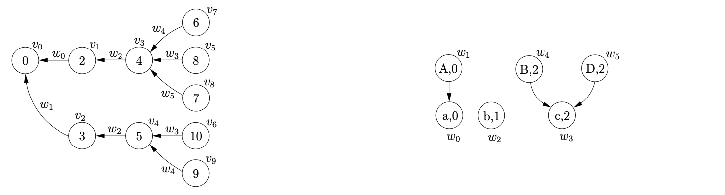
At this point $\mathcal{R}=\{(v_{3},B,1,0,w_{3}),(v_{3},D,1,0,w_{3})\}$ and $\mathcal{Q}=\{\}$. Processing $(v_{3},B,1,0,w_{3})$ results in the creation of node $v_{5}$ labelled $6$, the SPPF node $w_{4}$ and the edge between $v_{5}$ and $v_{3}$ labelled by $w_{4}$. The action in $\mathcal{T}(6,\$)$ is the reduction $r(S,4)$ so $(v_{3},S,4,0,w_{4})$ is added to $\mathcal{R}$. We then remove $(v_{3},D,1,0,w_{3})$ from $\mathcal{R}$ and process the reduction, which results in the GSS and SPPF shown in Figure 6.8 being constructed and $(v_{3},S,4,0,w_{5})$ added to $\mathcal{R}$.

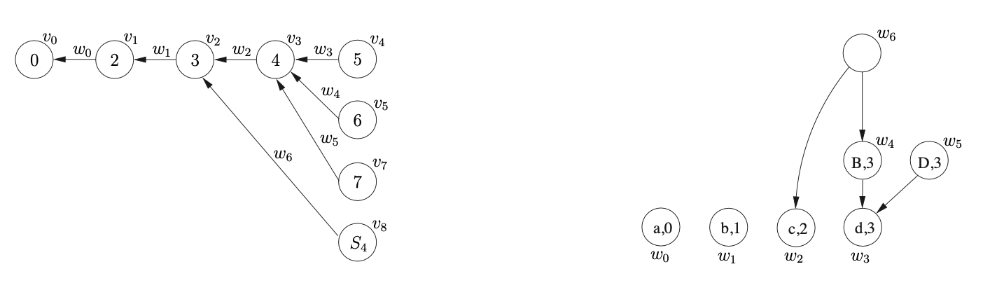
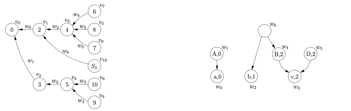
Since the next element, $(v_{3},S,4,0,w_{4})$, that we process from $\mathcal{R}$ has a reduction length greater than two, we collect the children and edges of the reduction’s source node, $v_{3}$, in the set $\chi=\{(v_{2},w_{2})\}$. We then create a new bookkeeping node $v_{8}$ labelled $S_{4}$ and the SPPF node $w_{6}$ which labels the new edge from $v_{8}$ to $v_{2}$. In order to ensure that the correct number of reduction steps are done we also add the binary reduction $(v_{2},S,3,0,w_{6})$ to $\mathcal{R}$. The only operation that remains to be done is to add the SPPF nodes collected in $\chi$ and the single node $y$, which is passed into the Reducer, as children of the new bookkeeping SPPF node $w_{6}$. We do this by calling the AddChildren function with the parameters $(w_{6},(w_{2},w_{4}),0)$. Since $w_{6}$ does not have any existing children, edges to $w_{2}$ and $w_{4}$ are created. The GSS and SPPF constructed up to this point are shown in Figure 6.9.

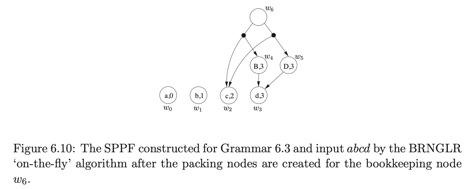
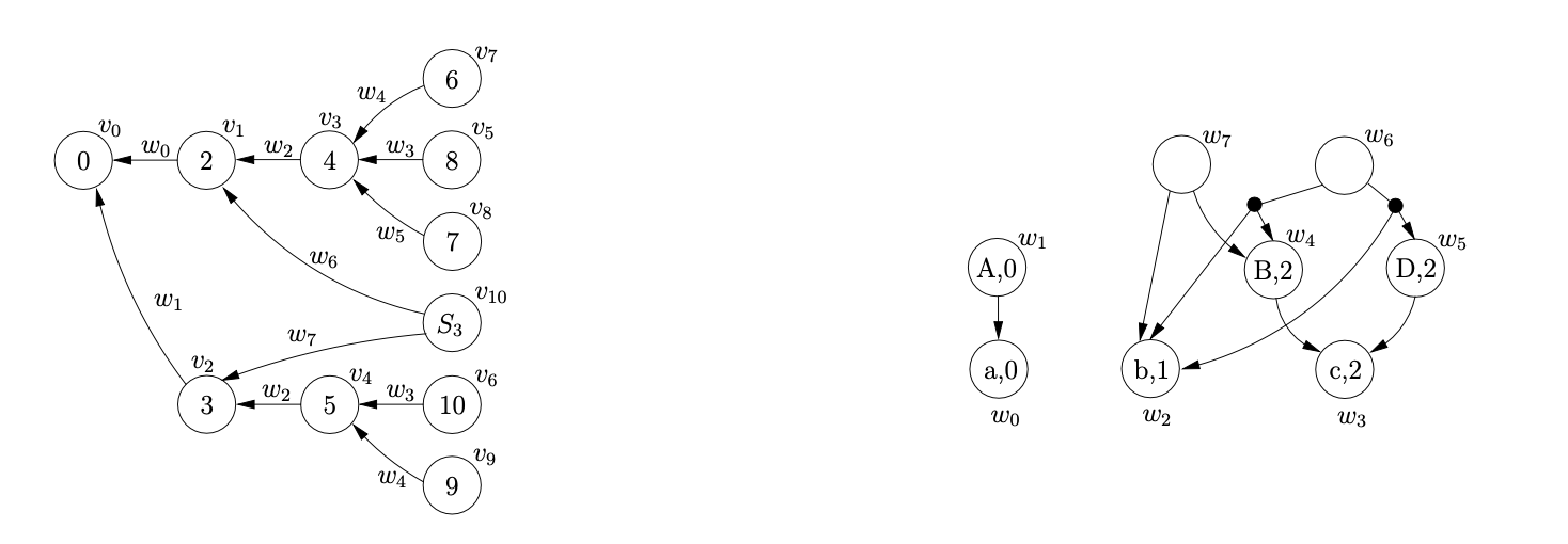
When we remove and process the reduction $(v_{3},S,4,0,w_{5})$ from $\mathcal{R}$ we proceed in the same way as before by collecting the children and edges of the reduction’s source node in the set $\chi=\{(v_{2},w_{2})\}$. However, since there already exists a node in the current level that is labelled $S_{4}$ we do not create a new one and since there is already an edge from $v_{8}$ to $v_{2}$ no edge is created either. Instead we make sure that the existing SPPF node $w_{6}$ has the correct children by calling AddChildren with the parameters $(w_{6},(w_{5},w_{2}),0)$.

Since $w_{6}$ has a sequence of children that is not labelled $(w_{5},w_{2})$ we create two new packing nodes as children of $w_{6}$ and add the two sequences of SPPF nodes to them as children. This results in the SPPF shown in Figure 6.10 being constructed.

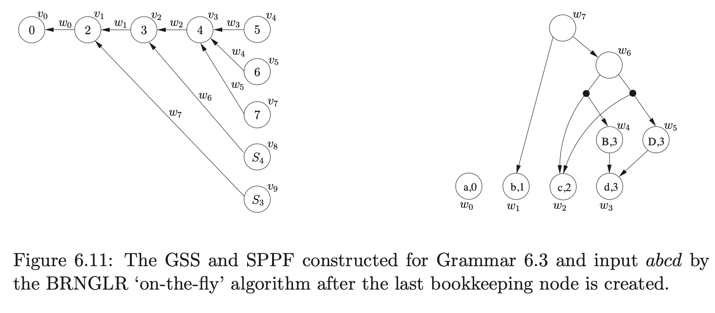
At this point $\mathcal{R}=\{(v_{2},S,1,0,w_{6})\}$ and $\mathcal{Q}=\{\}$. Processing $(v_{2},S,3,0,w_{6})$ we add $\{(v_{1},w_{1})\}$ to $\chi$ and since $m$ is greater than 2, we proceed to create a new node $v_{9}$ labelled $S_{3}$, a new SPPF node $w_{7}$ and an edge from $v_{9}$ to $v_{1}$ which is labelled by $w_{7}$. We then add $(v_{1},S,2,0,w_{7})$ for the final reduction step of the binary sequence of reductions to $\mathcal{R}$. Finally, we call AddChildren$(w_{7},(w_{6},w_{1}),0)$ which adds $w_{6}$ and $w_{1}$ as children of $w_{7}$ and results in the SPPF shown in Figure 6.11 being constructed.

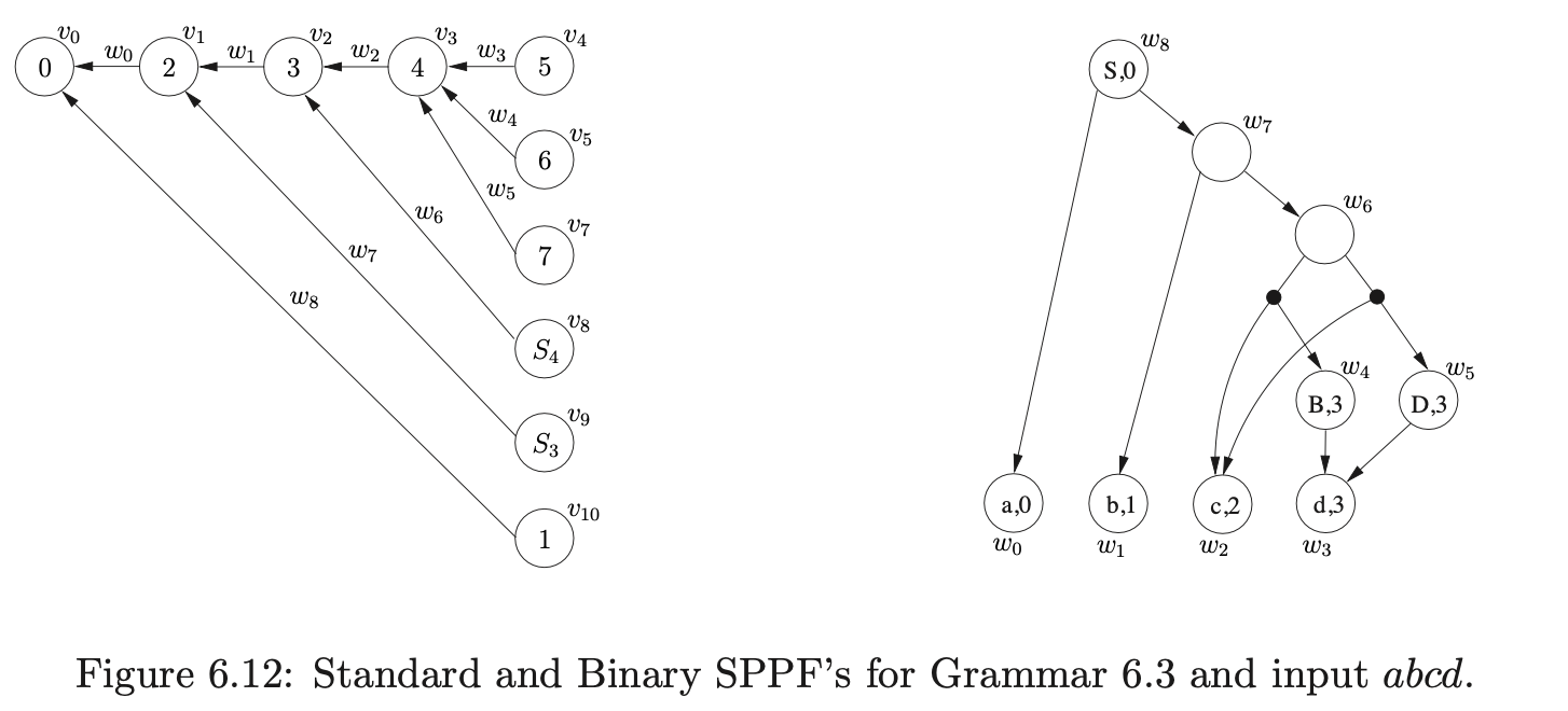
When we process $(v_{1},S,2,0,w_{7})$ we trace back to node $v_{0}$ and add $(v_{0},w_{0})$ to $\chi$. Since $m=2$ we recognise that this reduction will be completed in this step, so we find the goto action $p_{1}$ in $\mathcal{T}(0,S)$. We then create the new node $v_{10}$ labelled $1$ and the SPPF node $w_{8}$ labelled $(S,0)$, which we use to label the edge between nodes $v_{10}$ and $v_{0}$. The subsequent call to AddChildren with the parameters $(w_{8},(w_{0},w_{7}),0)$ results in the final SPPF shown in Figure 6.12 being constructed.

6.7 Packing of bookkeeping SPPF nodes¶

The previous section demonstrated how the ‘on-the-fly’ BRNGLR parsing algorithm builds an SPPF during parsing. At first it may appear that in general we could pack some of the bookkeeping nodes in the SPPF more effectively. In fact we cannot do this because incorrect derivations may be introduced to the SPPF. This section highlights the subtlety of packing bookkeeping nodes by tracing the construction of a GSS and SPPF for a grammar and string that will introduce incorrect derivations if the packing is done naively.

Example - how to pack bookkeeping SPPF nodes¶

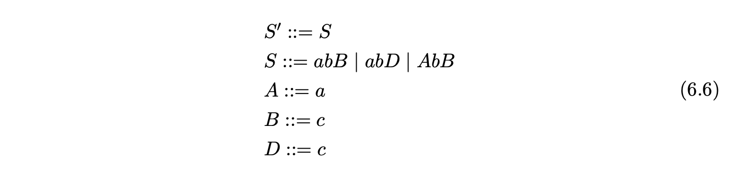
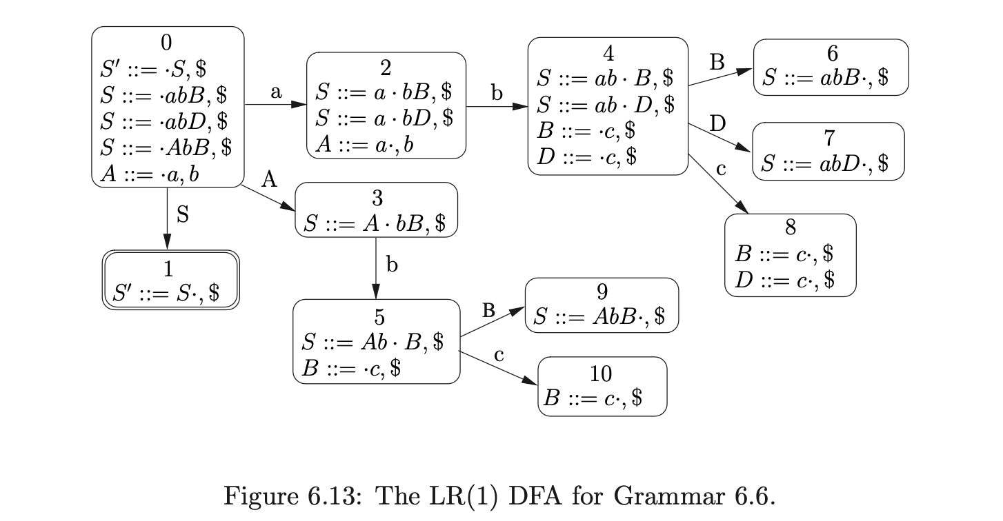
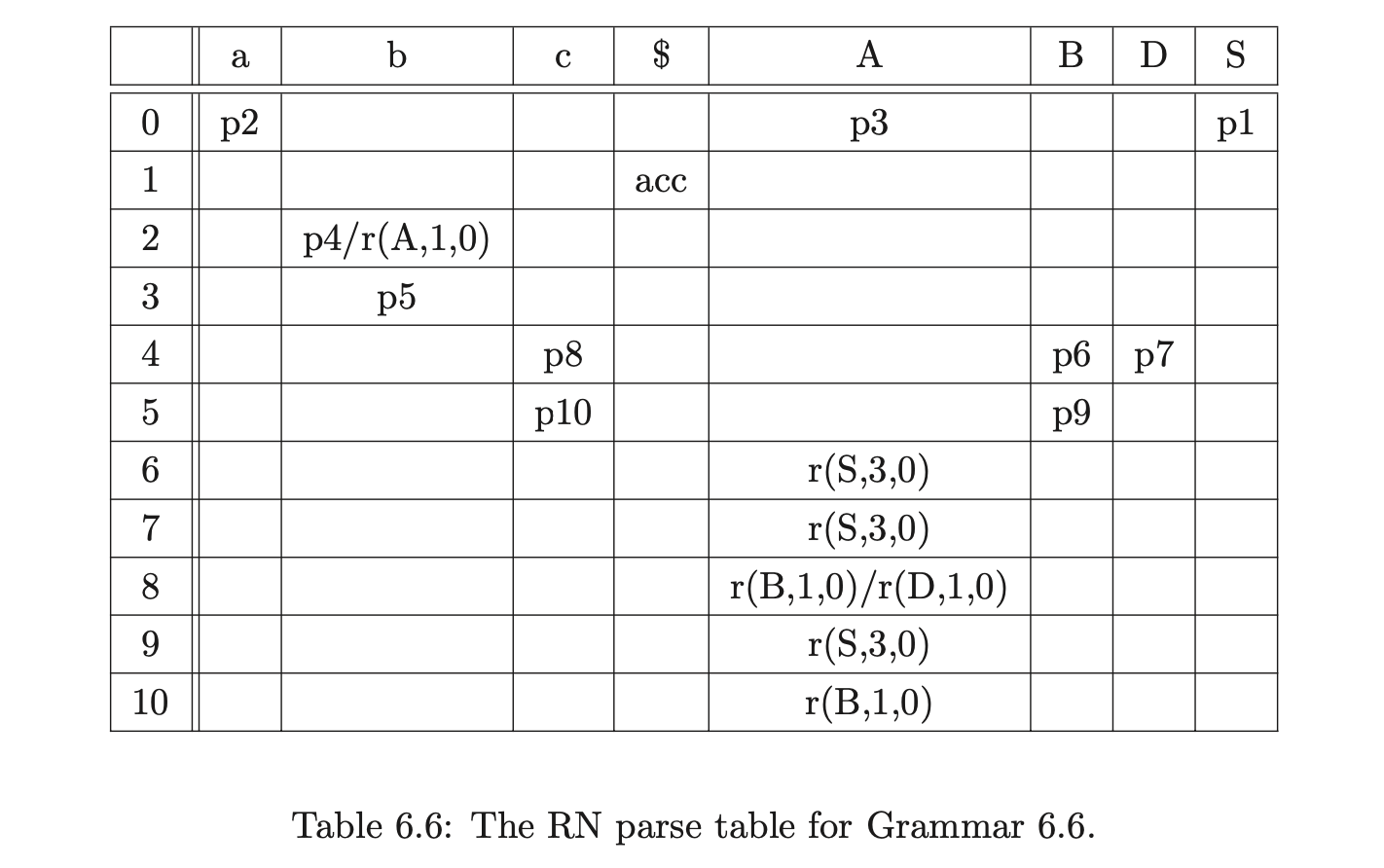
It is only possible to pack two bookkeeping SPPF nodes when they arise from different reductions whose target is the same state node. Consider Grammar 6.6, the LR(1) DFA in Figure 6.13 and RN parse table in Table 6.6. We can illustrate the consequences of incorrectly packing the bookkeeping SPPF nodes when parsing the string $abc$.

We begin in the usual way, creating the node $v_{0}$ labelled with the start state of the DFA and adding the actions from the associated parse table entry to the sets $\mathcal{R}$ and $\mathcal{Q}$. Since $p2$ is the only action in $\mathcal{T}(0,a)$ we shift the first input symbol and create a new node $v_{1}$ labelled $2$, an SPPF node $w_{0}$ labelled $(a,0)$ and an edge from $v_{1}$ to $v_{0}$ labelled by $w_{0}$. There is a shift/reduce conflict in the parse table at $\mathcal{T}(2,b)$ so $(v_{1},4)$ and $(v_{0},A,1,0,w_{0})$ are added to the sets $\mathcal{Q}$ and $\mathcal{R}$ respectively. Processing $(v_{0},A,1,0,w_{0})$ results in the node $v_{1}$ labelled $3$, the SPPF node $w_{1}$ labelled $(A,0)$ and the edge from $v_{1}$ to $v_{0}$ labelled by $w_{1}$ being created. Since the shift action $p5$ is in $\mathcal{T}(3,b)$, $(v_{2},5)$ is added to the set $\mathcal{Q}$. We then call the AddChildren function with the parameters $(v_{1},(w_{0}),0)$, which results in the SPPF node $w_{0}$ being added to $w_{1}$ as a child.

At this point, no other reductions are queued in the set $\mathcal{R}$ so the shifts are processed from the set $\mathcal{Q}$ by the Shifter. This results in the new nodes $v_{3}$ and $v_{4}$ being created, with edges to $v_{1}$ and $v_{2}$ labelled by the newly created SPPF node $w_{2}$. Both nodes $v_{3}$ and $v_{4}$ only have shift actions in their respective parse table entries so the new nodes $v_{5}$ and $v_{6}$ are created along with the associated SPPF node $w_{3}$.

At this point $\mathcal{R}=\{(v_{3},B,1,0,w_{3}),(v_{3},D,1,0,w_{3}),(v_{4},B,1,0,w_{3})\}$ and $\mathcal{Q}=\{\}$. Processing the first element in $\mathcal{R}$ results in the new node $v_{7}$ labelled $6$, the SPPF node $w_{4}$ labelled $(B,2)$ and the edge from $v_{7}$ to $v_{3}$ being created. Since the length of the reduction is one, we find the new reduction $r(S,3,0)$ in $\mathcal{T}(6,\$)$ and add $(v_{3},S,3,0,w_{4})$ to $\mathcal{R}$ before proceeding to call AddChildren$(w_{4},(w_{3}),0)$ which makes $w_{3}$ a child of $w_{4}$ in the SPPF.

When we remove $(v_{3},D,1,0,w_{3})$ from $\mathcal{R}$ and continue to process the reduction in the Reducer, we create the new node $v_{8}$ labelled $7$, the SPPF node $w_{5}$ labelled $(D,2)$ and the edge between $v_{8}$ and $v_{3}$ labelled by $w_{5}$. The new reduction $(v_{3},S,3,0,w_{5})$ is added to $\mathcal{R}$ and then AddChildren$(w_{5},(w_{3}),0)$ is called which results in $w3$ being made a child of $w_{5}$.

Then we remove $(v_{4},B,1,0,w_{3})$ from $\mathcal{R}$ which results in the node $v_{9}$ labelled $9$ being created in the GSS. Since an edge does not already exist from $v_{9}$ to $v_{4}$ one is created. However, because we have already created an SPPF node labelled $(B,2)$ while constructing the current level, which we find in the set $\mathcal{N}$, we reuse it to label the new edge. In addition to this because the parse table contains the reduction $r(S,3,0)$ in $\mathcal{T}(9,\$)$, we add $(v_{4},S,3,0,w_{5})$ to $\mathcal{R}$.

We then continue processing the remaining reductions $(v_{3},S,3,0,w_{4})$, $(v_{3},S,3,0,w_{5})$ and $(v_{4},S,3,0,w_{5})$ from the set $\mathcal{R}$. For $(v_{3},S,3,0,w_{4})$ the Reducer determines that the length of the reduction is greater than two and proceeds to perform a binary reduction. The child node and edge $(v_{1},w_{2})$, from node $v_{3}$ are found and added to the set $\chi$. A new bookkeeping node $v_{10}$ labelled $S_{3}$ is then created and an edge is added between $v_{10}$ and $v_{1}$. The final binary reduction of the sequence $(v_{1},S,2,0,w_{6})$ is also added to $\mathcal{R}$ before the SPPF is updated by AddChildren$(w_{6},(w_{2},w_{4}),0)$.

When $(v_{3},S,3,0,w_{5})$ is processed, another binary reduction is performed by the Reducer. Once again the child node and edge $(v_{1},w_{2})$, from node $v_{3}$ are found and added to the set $\chi$. However, since there is already a node in the current level that is labelled $S_{3}$, we do not create a new one, but reuse the existing one. In addition to this, because there is already an edge between $v_{10}$ and $v_{1}$, we also reuse the edge and SPPF node. When we finally call AddChildren$(w_{6},(w_{2},w_{5}),0)$, we find that two new packing nodes need to be created as children of $w_{6}$. So we add the original sequence of children to one packing node and the new sequence that is passed into AddChildren to the other.

When we process $(v_{4},S,3,0,w_{5})$, another binary reduction is performed. We begin by setting $\chi=\{(v_{2},w_{2})\}$. Since we already have a node labelled $S_{3}$ in the current level of the GSS, we can use it again. However, because there is no edge that goes between $v_{10}$ and $v_{2}$, we create a new one and label it with a new SPPF node $w_{7}$. Before calling the AddChildren function we add the remaining binary reduction $(v_{2},S,2,0,w_{7})$ to $\mathcal{R}$.

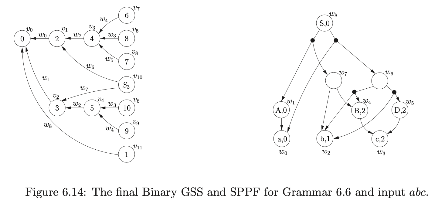
Processing the final two reductions, $(v_{1},S,2,0,w_{6})$ and $(v_{2},S,2,0,w_{7})$, held in $\mathcal{R}$ results in the node $v_{11}$ being created in the GSS that is labelled with the accepting state of the DFA. Since $v_{11}$ is in the final level of the GSS, the string $abc$ is accepted by the parser. The final GSS and SPPF constructed by the BRNGLR parsing algorithm are shown in Figure 6.14.

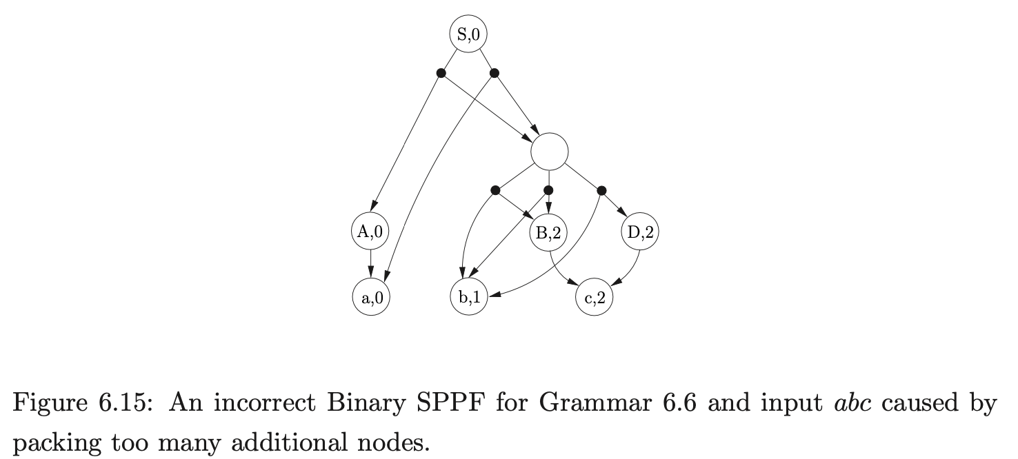
At first, it may appear that it is possible to pack the two SPPF nodes $w_{6}$ and $w_{7}$ to produce the more compact SPPF shown in Figure 6.15. Unfortunately if this is done the following incorrect ‘derivation’ will be included.

\[S^{\prime}\Rightarrow S\Rightarrow AbD\Rightarrow abD\Rightarrow abc\]

6.8 Summary¶

In this chapter we have presented an algorithm capable of parsing all context-free grammars in at most $O(n^{3})$ time and space. Two versions of the recognition algorithm were presented. The first worked on modified RN parse tables which included new states and reduction actions to ensure reductions of at most length two were done. The second algorithm used RN parse tables and split reductions with lengths $m>2$ into $m-1$ reductions of length 2 ‘on-the-fly’. This did not require any modifications to be done to the parse table or the grammar, and hence did not increase the size of the parser. The ‘on-the-fly’ recognition algorithm was then extended to a parser which is able to construct an SPPF representation of all possible derivations for a given input string in at most cubic time and space. Proofs of the correctness of the algorithms and their complexity analysis can be found in [13]. Chapter 10 presents the experimental results for grammars which trigger worst case performance and several programming language grammars and strings. The results corroborate the complexity analysis and provide an encouraging comparison between BRNGLR and other general parsing algorithms. The next chapter presents another general parsing algorithm that achieves cubic worst case time complexity by minimising the amount of stack activity that is done during parsing.