10. Experimental investigation

This chapter presents the experimental results based on eight of the generalised parsing algorithms described in this thesis: RNGLR, BRNGLR, RIGLR, Tomita1e, Tomita1e modified, Farshi naive, Farshi optimised and Earley. Several pathological grammars are used to trigger the algorithms’ worst case behaviour and three programming language grammars are used to gauge their performance in practice. All the algorithms’ results are given for the recognition time and space required, while the RNGLR and BRNGLR results include statistics on the SPPF construction.

10.1 Overview of chapter

In Chapter 4 we discussed Tomita’s GLR parsing algorithms, specifically focusing on his Algorithm 1, that only works for \(\epsilon\)-free grammars, and Farshi’s extension that works for all grammars. We have implemented Farshi’s algorithm exactly as it is described in [10], and we have also implemented a more efficient version which truncates the searches in the GSS as described in Chapter 4. We refer to the former as Farshi-naive and the latter as Farshi-opt. We present the results for both algorithms in Section 10.6.

In Chapter 5 we discussed a minor modification, Algorithm 1e, of Tomita’s Algorithm 1, which admits grammars with \(\epsilon\)-rules. On right nullable grammars, Algorithm 1e performs less efficiently with RN parse tables than LR(1) parse tables (although of course sometimes it performs incorrectly on LR(1) tables). We have a modified algorithm (Algorithm 1e mod) which is actually more efficient on RN tables than Algorithm 1e is on the LR(1) table.

We now present experimental data comparing the performance of the different algorithms. RNGLR is compared to Farshi, as these are the two fully general GLR algorithms. However, even with the modifications mentioned above, Farshi’s algorithm is not as efficient as Tomita’s algorithm, thus the RNGLR algorithm is also compared to Tomita’s original approach using Algorithm 1e.

The BRNGLR algorithm is asymptotically faster than the RNGLR algorithm in worst case and data showing this is given. Experiments are also carried out on average cases using Pascal, Cobol and C grammars, to investigate typical as well as worst case performance. The BRNGLR algorithm is also compared to Earley’s classic cubic general parsing algorithm and to the cubic RIGLR algorithm, as this was designed to have reduced constants of proportionality by limiting the underlying stack activity.

We also present data comparing the relative efficiency of the GLR algorithms when different types (LR(0), SLR(1), LALR(1) and LR(1)) of parse table are used.

10.2 The Grammar Tool Box and Parser Animation Tool

The Grammar Tool Box (GTB) [15] is a system for studying language specification and translation. GTB includes a set of built-in functions for creating, modifying and displaying structures associated with parsing.

The Parser Animation Tool (PAT) is an accompanying visualisation tool that has its own implementations of the parsing algorithms discussed in this thesis which run from tables generated by GTB. PAT is written in Java, and GTB in C++ so they necessarily require separate implementations, but this has the added benefit of two authors constructing independent programs from the theoretical treatment. PAT dynamically displays the construction of parse time structures and can also be used in batch mode to generate statistics on parser behaviour. The results presented in this chapter have been generated in this way. A guide to PAT and its use is given in Appendix A.

The complete tool chain conducted for this thesis comprises of ebnf2bnf, a tool for converting extended BNF grammars to BNF; GTB which is used to analyse grammars and construct parse tables, and PAT which is used to animate algorithms and generate statistics on parse-time structure size.

10.3 The grammars

Pascal and C typify the top-down and bottom-up approaches to language design. In folklore at least, Pascal is thought of as being designed for LL(1) parsing and C for LALR(1) parsing. In practice, Pascal is reasonably close to LL(1). Our Pascal grammar only has one SLR(1) conflict, arising from the if-then-else ambiguity. C is essentially parsable with an LALR(1) parser, but was not initially designed that way. The LALR(1) ANSI-C grammar was only written by Tom Penello in about 1983. Bjarne Stroustrup described at some length the difficulties involved in attempting to build parsers for early versions of C++ using a hybrid of Yacc and a lexer containing much lexical trickery relying on recursive descent techniques [12, p.68]. C++’snon-deterministic syntax has clearly stimulated the development of tools such as ANTLR [11] and the GLR mode of Bison [12]. Cobol’s development was contemporary with that of Algol-60 and thus pre-dates the development of deterministic parsing techniques. The language has a large vocabulary which will challenge any table based parsing method.

For these experiments we have used the grammar for ISO-7185 Pascal extracted from the standard, the grammar for ANSI-C extracted from [10] and a grammar for IBM VS-Cobol developed in Amsterdam. This grammar is described in [11]. A version of the grammar is available as a hyperlinked browsable HTML file from [Cob]: we used a version prepared for Asf+Sdf from which we extracted the context-free rules. The original grammars are written in EBNF. The ebnf2bnf tool was used to generate corresponding BNF grammars. See [12] for more details of this tool.

To demonstrate the non-cubic behaviour of the RNGLR, Farshi and Tomita 1e algorithms we have used Grammar 6.1 (see page 118), which is discussed in detail in Chapter 6.

10.4 The input strings

For all the input strings used in the experiments we have suppressed lexical level productions and used separate tokenisers to convert source programs into strings of terminals from the main grammar. For instance the Pascal fragment

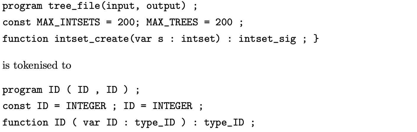
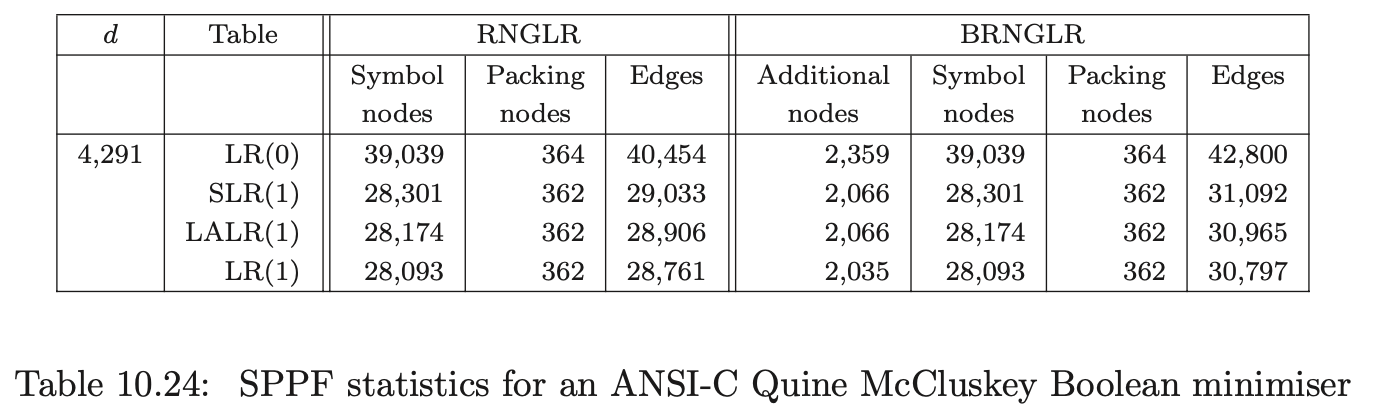
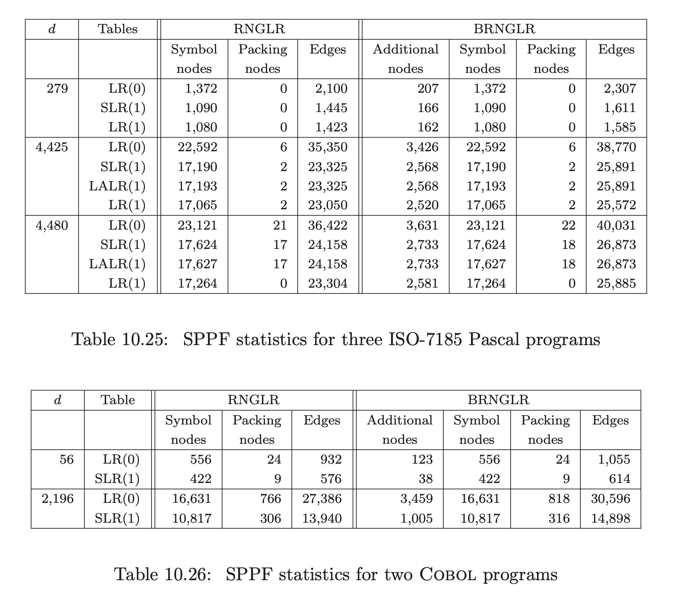
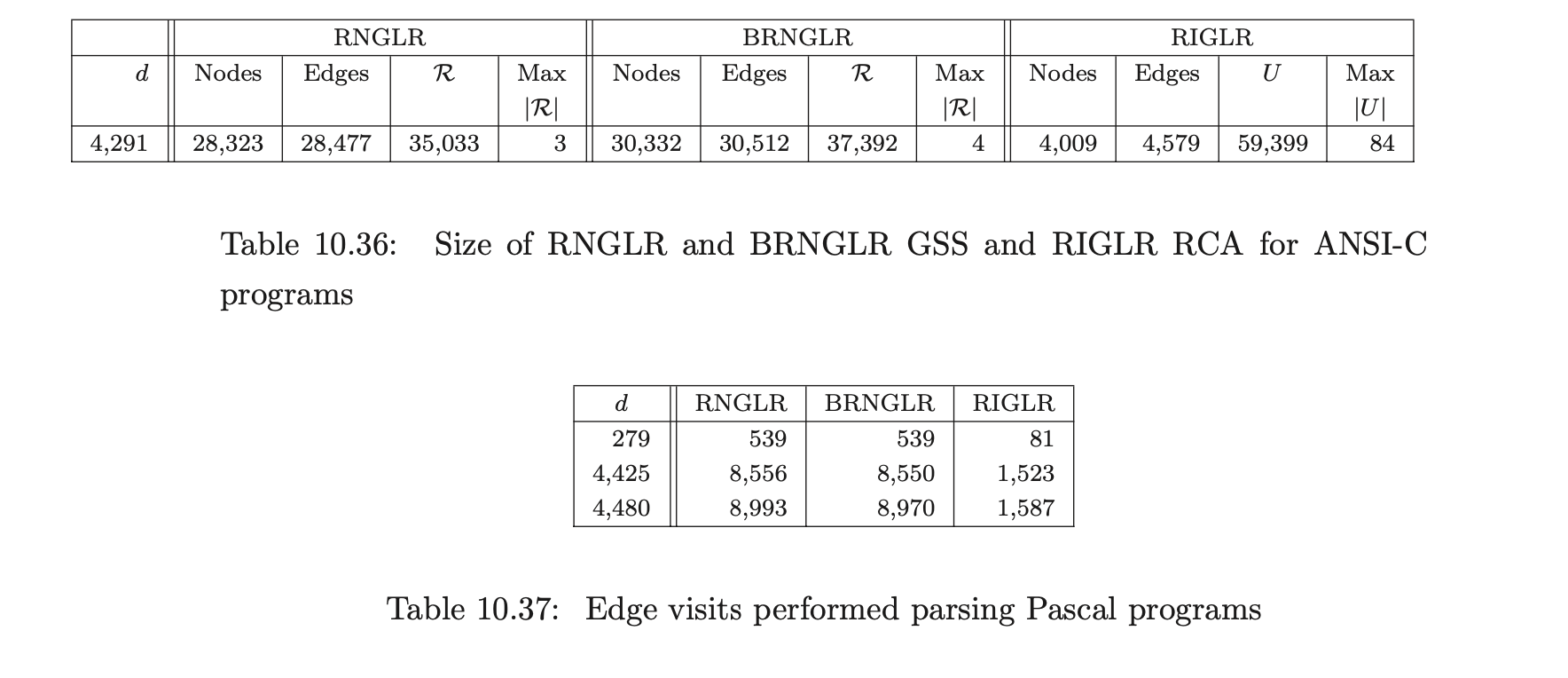
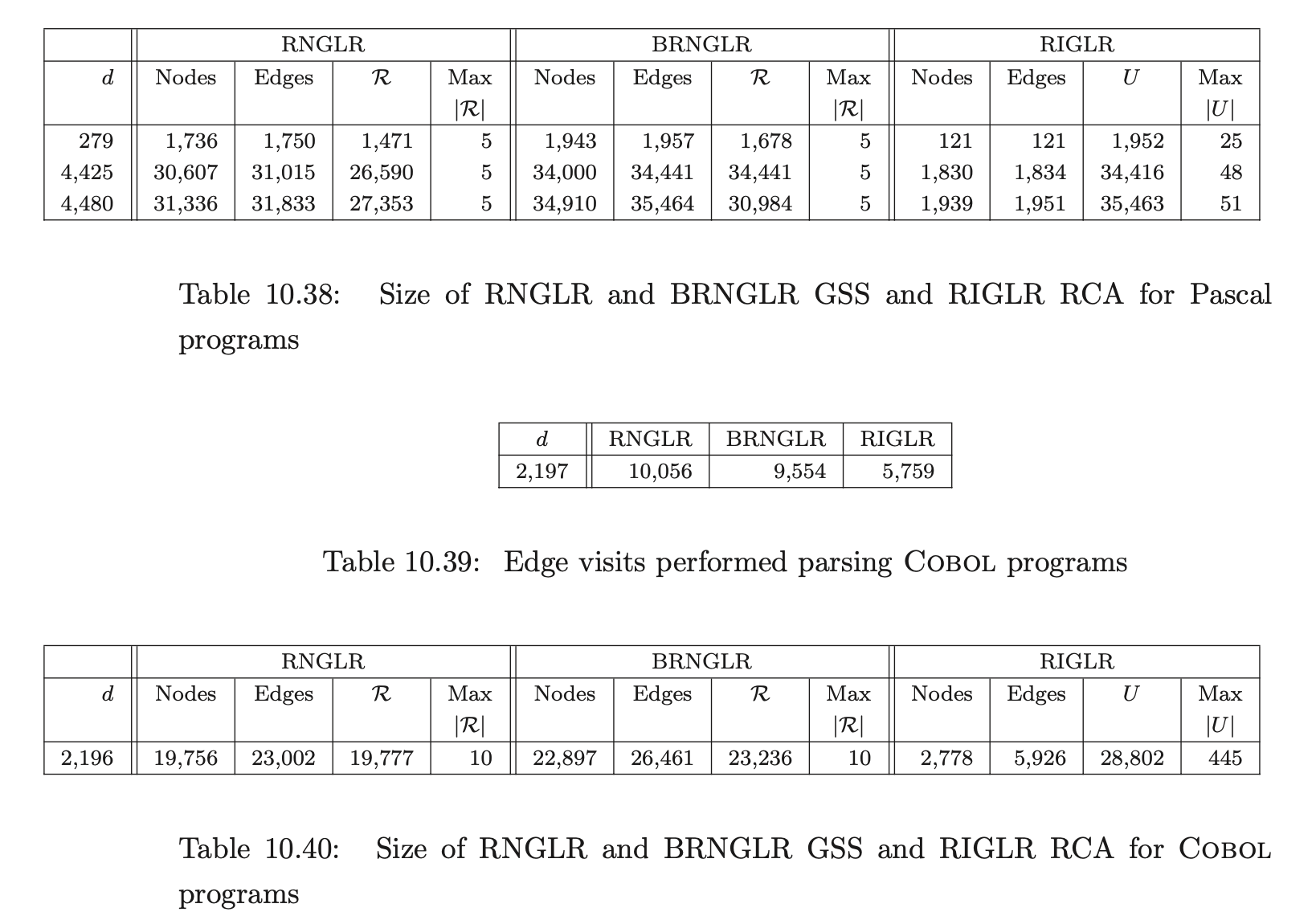
For Pascal, our source was two versions of a tree viewer program with 4,425 and 4,480 tokens respectively, and a quadratic root calculator with 429 tokens; for ANSI-C a Boolean equation minimiser of 4,291 tokens; and for Cobol, two strings extracted from the test set supplied with the grammar consisting of 56 and 2,196 tokens respectively.

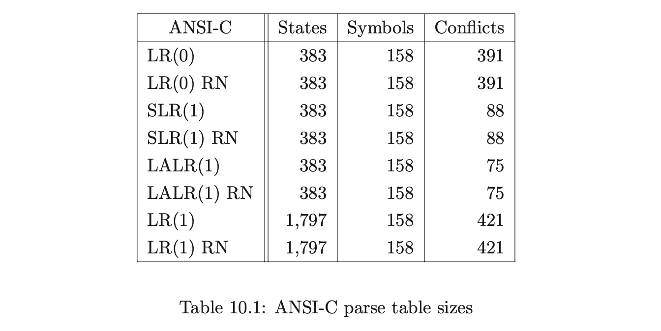
The tokeniser’s inability to distinguish between identifiers and type names in C has meant that our C grammar does not distinguish them either. This is the reason for the high number of LR(1) conflicts in the grammars.

The parses for Grammar 6.1 are performed on strings of \(b\)’s of varying lengths.

10.5 Parse table sizes

This section compares the sizes of the LR(0), SLR(1), LALR(1) and LR(1) parse tables with the corresponding RN tables for our ANSI-C, Pascal and Cobol grammars.

Recall from Chapter 5 that the RNGLR algorithm corrects the problem with Tomita’s Algorithm 1e by performing nullable reductions early. This is achieved through the modification of the LR parse table. For a given combination of grammar and LR(0), SLR(1), LALR(1), or LR(1) parse table, the GSS constructed during a parse will be the same size for both RN- and conventional Knuth-style reductions. In general the RN tables will contain far more conflicts, which might be expected to generate more searching during the GSS construction. In Section 10.6 we shall show that, contrary to intuition, the RNGLR algorithm performs better than either Tomita or Farshi’s algorithms. In fact it reduces the stack activity compared to the standard LR parsing algorithm for grammars that contain right nullable rules. The LR(0), SLR(1), LALR(1), LR(1), and RN parse tables for each of the programming language grammars are shown in Tables 10.1, 10.2 and 10.3.

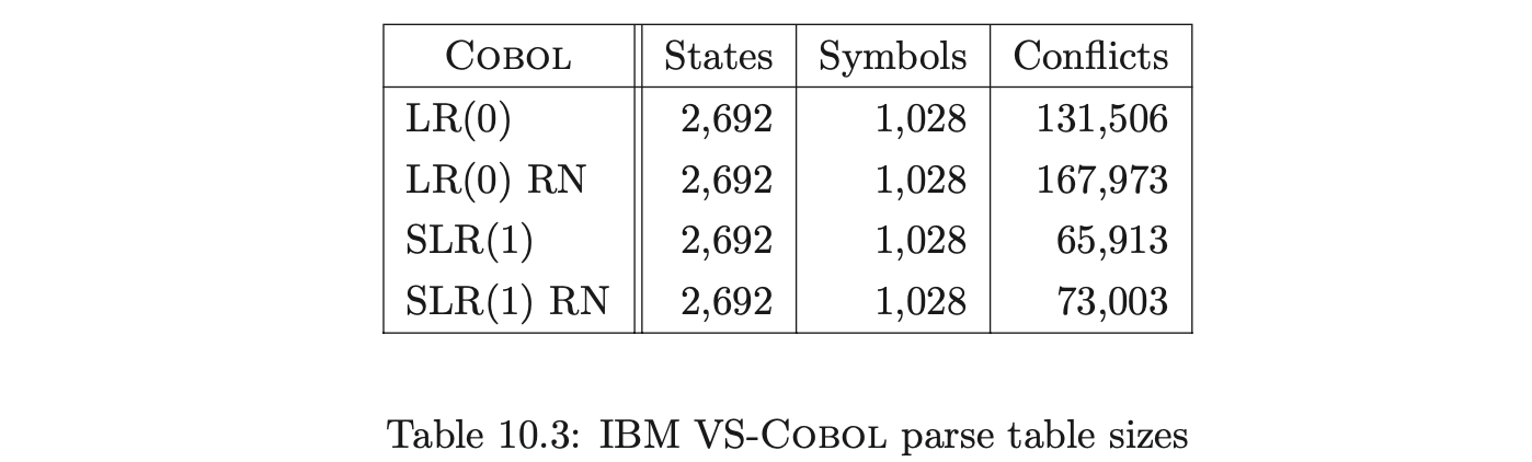
Coвol requires more than seven times as many states as ANSI-C for LR(0) and SLR(1) tables. In fact GTB’s LR(1) table generator ran out of memory when processing CoBOL, so we leave those entries empty. GTB builds LALR(1) parse tables by merging \(\operatorname{LR}(1)\) tables so those entries for CoBOL are also blank. We see that this CоBOL grammar is highly non-deterministic, reflecting the construction process described in [LV01]. We now consider how the use of different parse tables affects the size of the GSS constructed by our GLR algorithms. Tables 10.4, 10.5 and 10.6 present the number of GSS nodes and edges created during the parse of the C, Pascal and CoBoL input strings respectively.

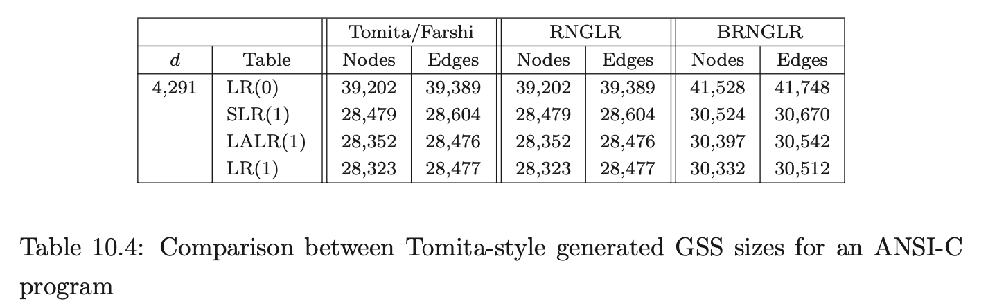
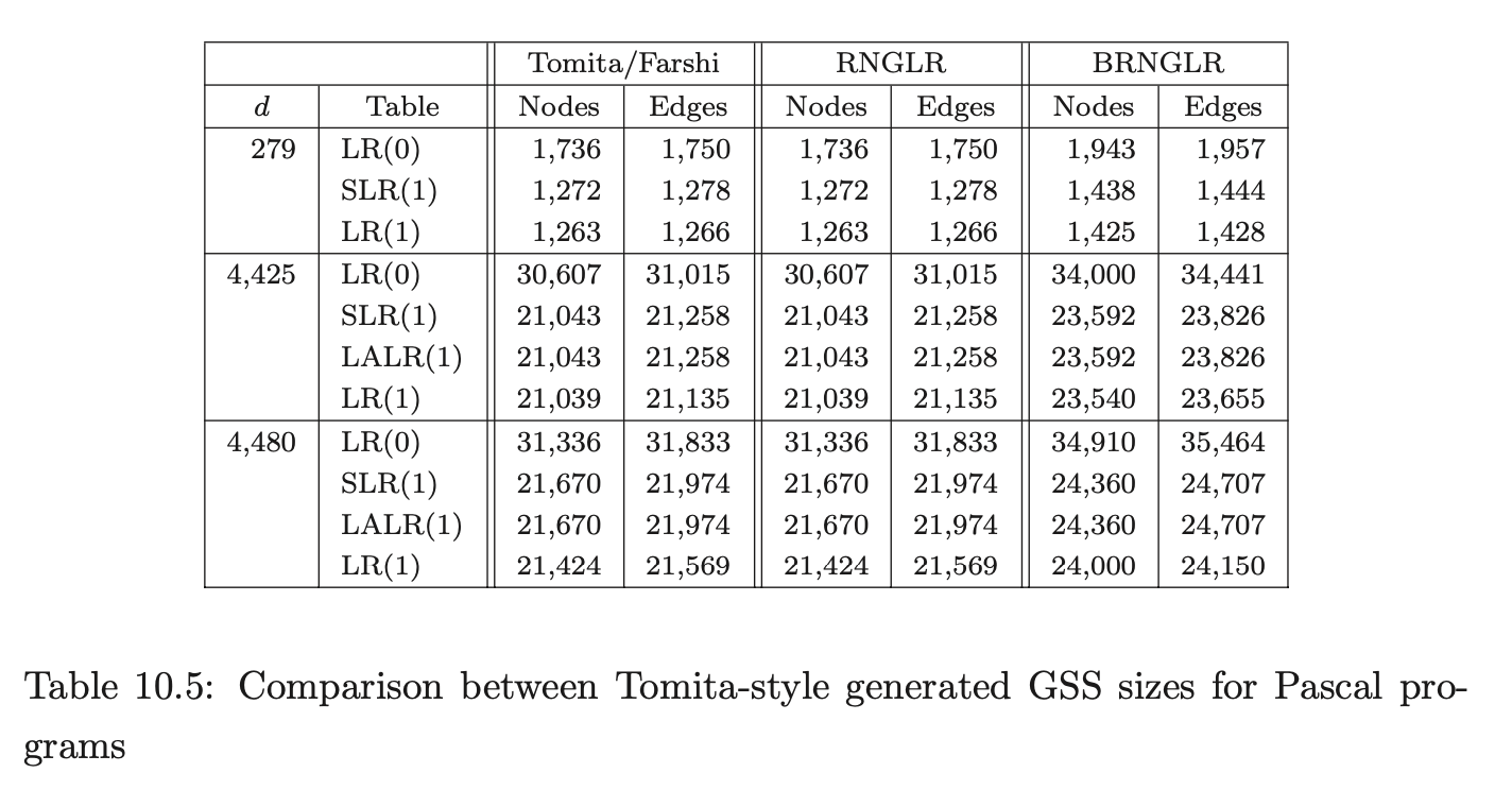
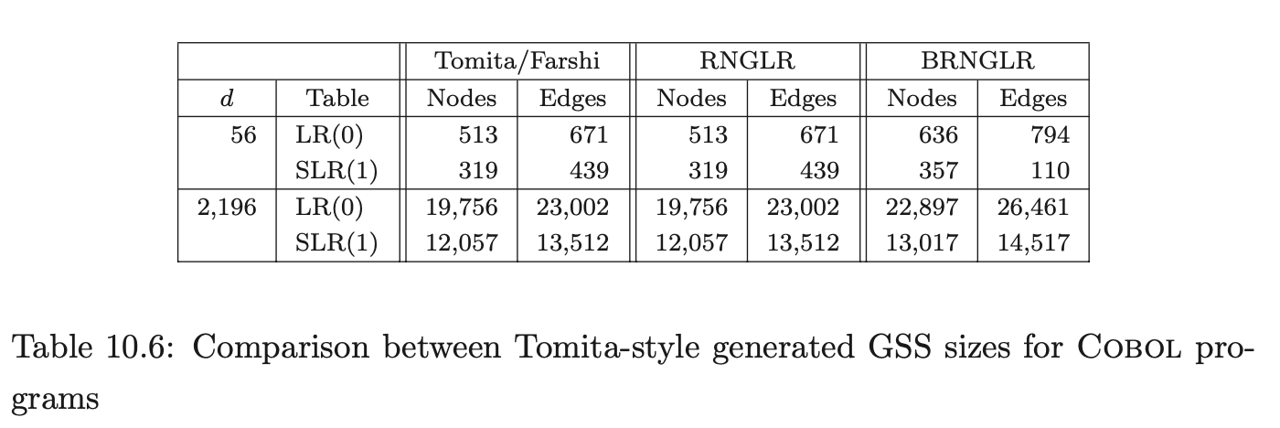
The Tomita, Farshi and RNGLR algorithms generate the same structures. The BRNGLR algorithm achieves cubic run times but at the cost of a worst-case constant factor increase in the size of the structures. For any grammar with productions greater than two symbols long the BRNGLR algorithm introduces additional nodes into the GSS. The results show increases of around 10 % in the size of the structures. There is a potential trade off between the amount of nondeterminism in the table and the size of the GSS. Some early reports, [Lan91], [BL89], suggest that LR(1) based GSS’s would be much larger than SLR(1) ones because the number of states is so much larger, and in the limit, the number of nodes in a GSS is bounded by the product of the number of table states and the length of the string. However, this is not necessarily the case. The above tables show LR(1) GSS’s that are a little smaller than the corresponding SLR(1) ones. Of course, the LR(1) tables themselves are usually much bigger than SLR(1) tables so the rather small reduction in GSS size might only be justified for very long strings. The AsF+SDF Meta Environment uses SLR(1) tables. In the next section we turn our attention to the performance of the GLR algorithms and show how the use of different parse tables affects the performance of the Tomita, Farshi and RNGLR algorithms. Of course, there are pathological cases where the size of an LR(1) GSS is much greater than the corresponding SLR(1) GSS. See [JSE04b].

10.6 The performance of the RNGLR algorithm compared to the Tomita and Farshi algorithms

Tomita’s Algorithm 1 was only designed to work on \(\epsilon\)-free grammars. We have presented a straightforward extension to his algorithm to allow it to handle grammars containing \(\epsilon\)-rules. Unfortunately this extended algorithm, which we have called Algorithm 1e, may fail to correctly parse grammars with hidden-right recursion. As mentioned in Section 10.1 we have discussed a slightly more efficient version, Algorithm 1e mod, of Algorithm 1e.

In Chapter 5 we discussed the RNGLR algorithm and showed how it extends Tomita’s Algorithm 1 to parse all context-free grammars. Our technique is not the first attempt to fully generalise Tomita’s algorithm (see Chapter 4). Farshi presented a ‘brute-force’ algorithm which handles all context-free grammars. However, his approach introduces a lot of extra searching. Here we compare the efficiency of Farshi’s algorithm with the RNGLR algorithm. Because Farshi’s algorithm is not efficient we also compare RNGLR with Algorithm 1e.

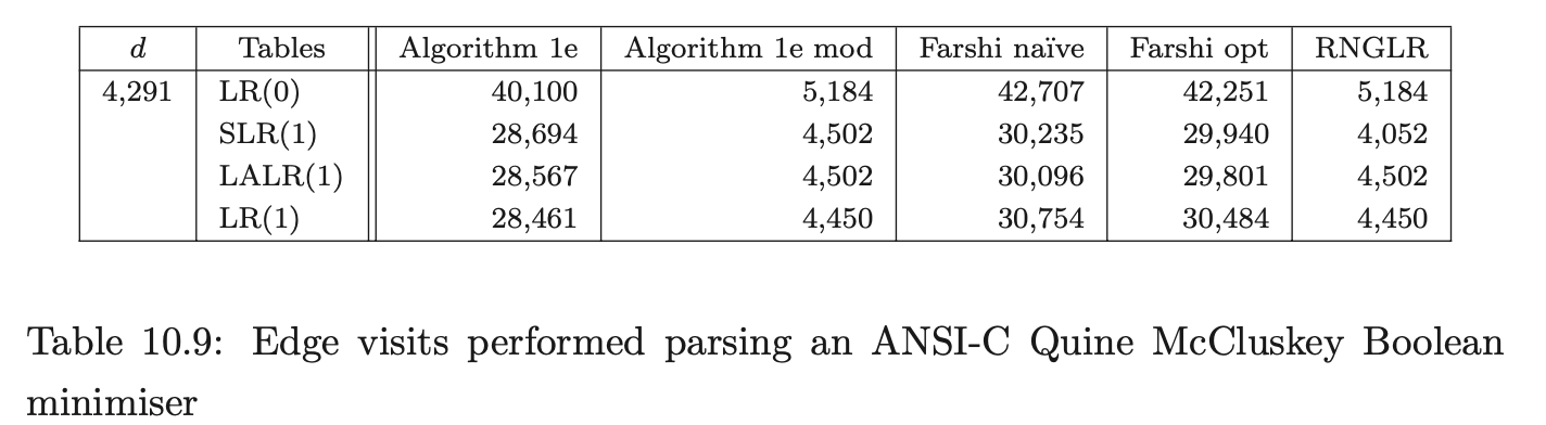
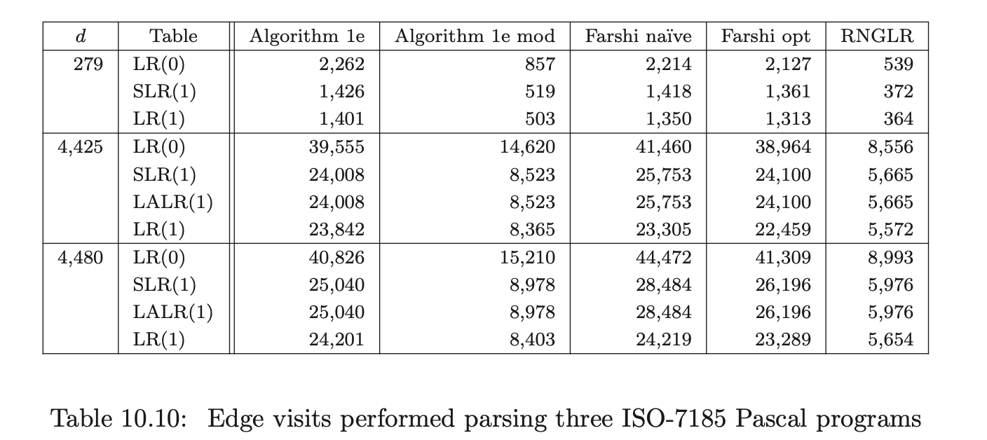
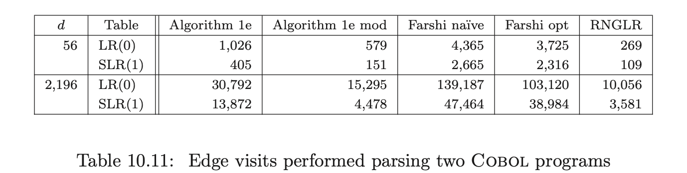
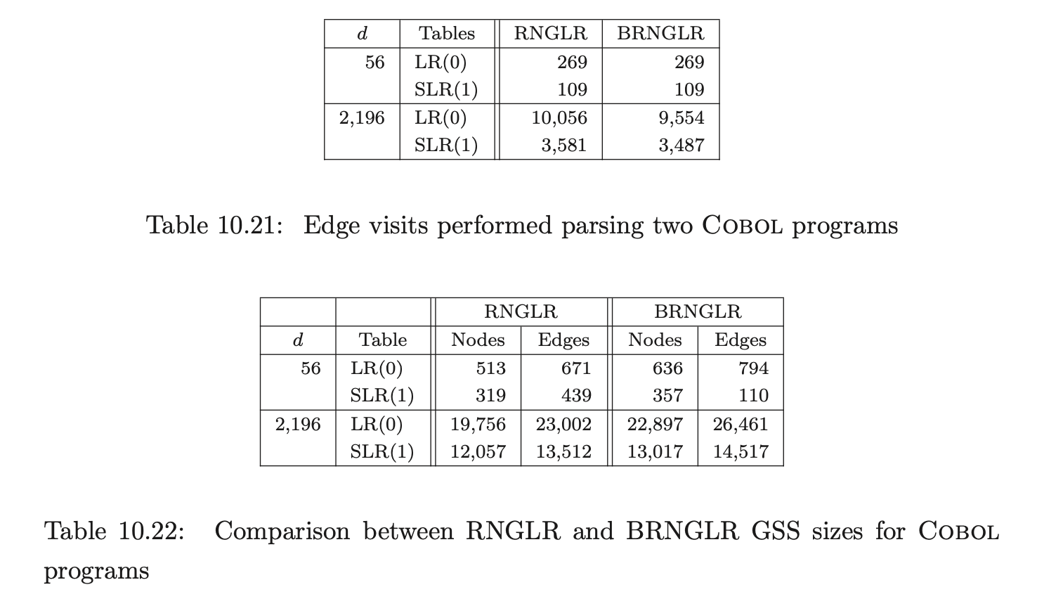
To compare the efficiency of the GSS construction between the different algorithms, the number of edge visits performed during the application of a reduction are counted. An edge visit is only counted when tracing back all possible paths during a reduction. The creation of an edge is not counted as an edge visit. Recall that in the RNGLR and Algorithm 1e mod algorithms the first edge in a reduction path is not visited because of the way pending reductions are stored in the set \(\mathcal{R}\).

A non-cubic example

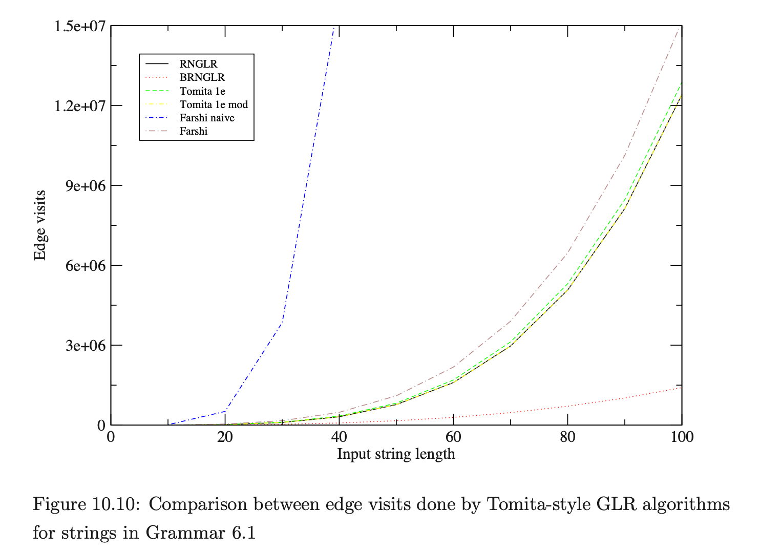
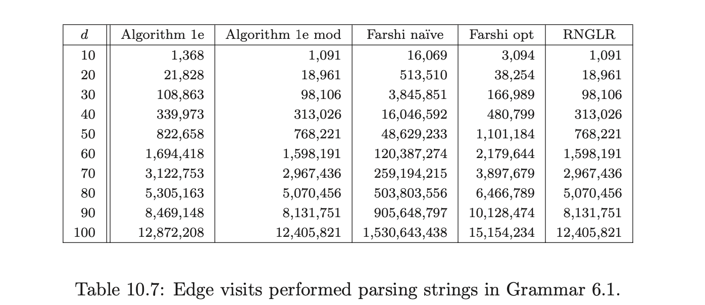
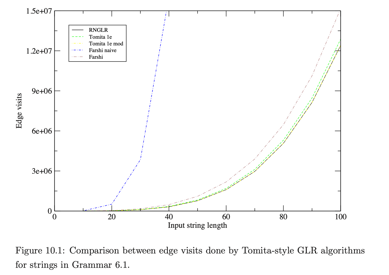
We begin by discussing the results for parses of strings \(b^{d}\) in Grammar 6.1. This grammar has been shown to trigger worst case behaviour for the GLR-style algorithms (see Chapter 6). 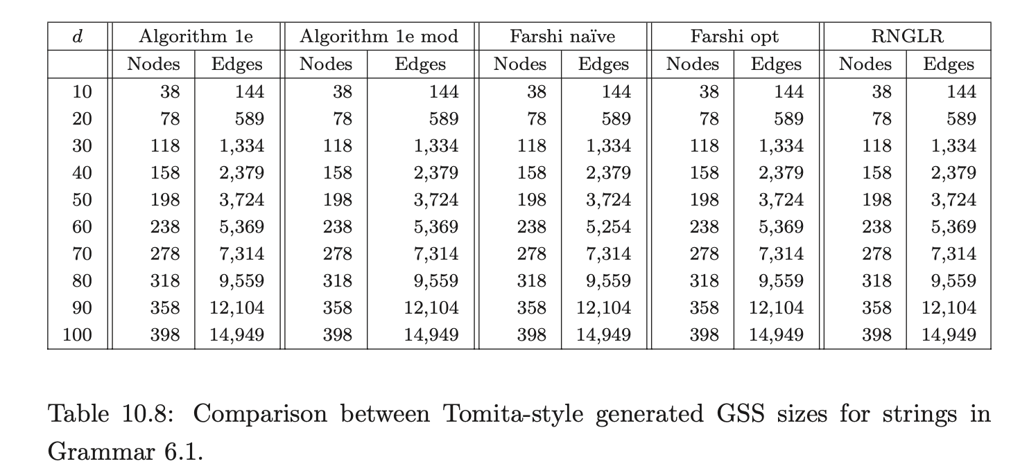As we can see, all of the algorithms perform badly as expected, but Farshi’s naive version is much worse than the others. However, the GSS produced by each of the algorithms should be the same and the figures in Table 10.8 support this expectation.

10.6.2 Using different LR tables

In this section we compare the GSS construction costs when different types of LR tables are used.

GTB and PAT have allowed us to make direct comparisons between the Tomita, Farshi and RNGLR algorithms and three types of LR table. In all cases the LR(1) table resulted in smaller and faster run-time parsers, but the improvement over SLR(1) is not very big, while the increase in the size of the table is significant. Of course, there are pathological cases where the size of an LR(1) GSS is much greater than the corresponding SLR(1) GSS. For example, consider Grammar 10.1 and Grammar 10.2. Both grammars illustrate situations in which all three DFA types are equally bad, but the LR(1) tables result in smaller GSS’s being constructed than for the SLR(1) tables.

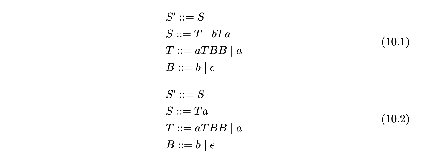
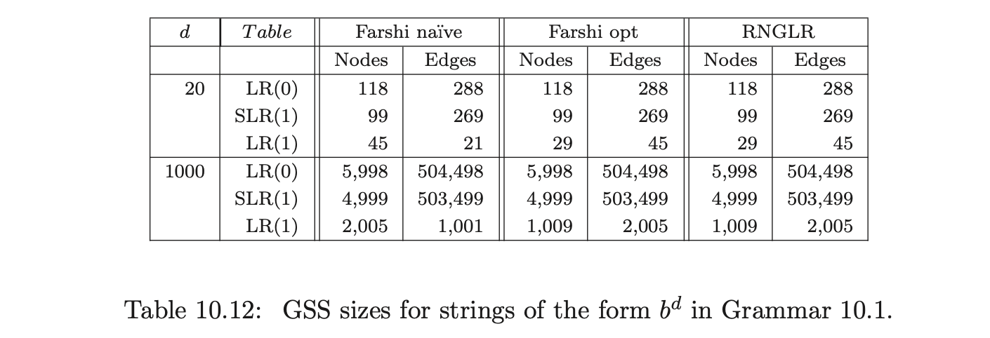
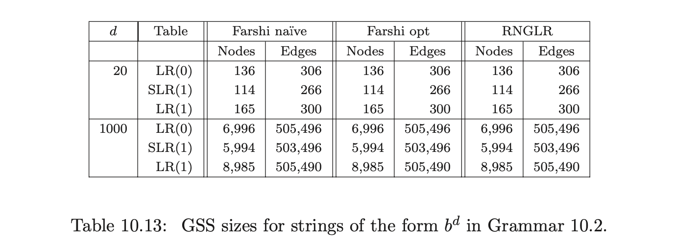
Table 10.14 shows that there is a significant difference in the run-time cost of a parse for Grammars 10.1 using the LR(1) parse table compared to the SLR(1) and LR(0) parse tables.

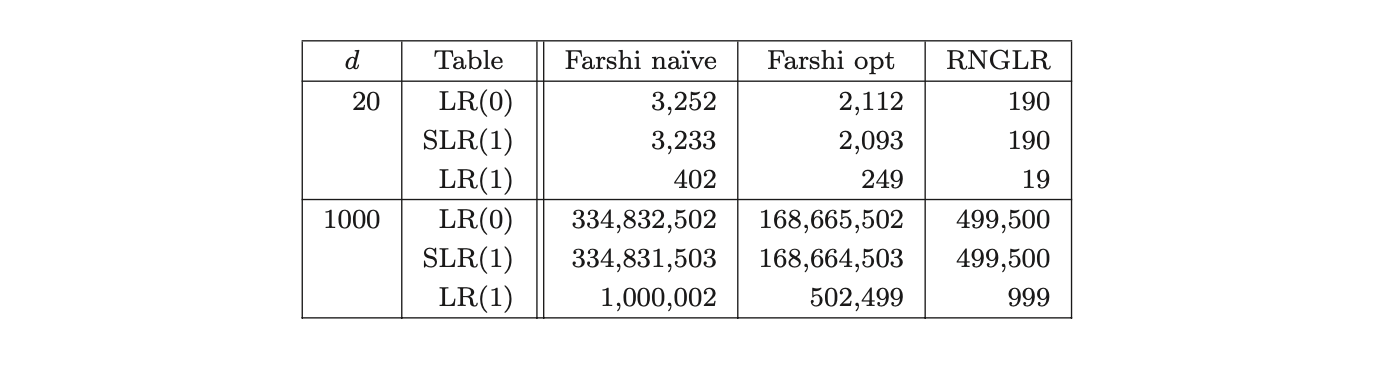Table 10.14: Edge visits performed parsing strings of the form bd in Grammar 10.1. 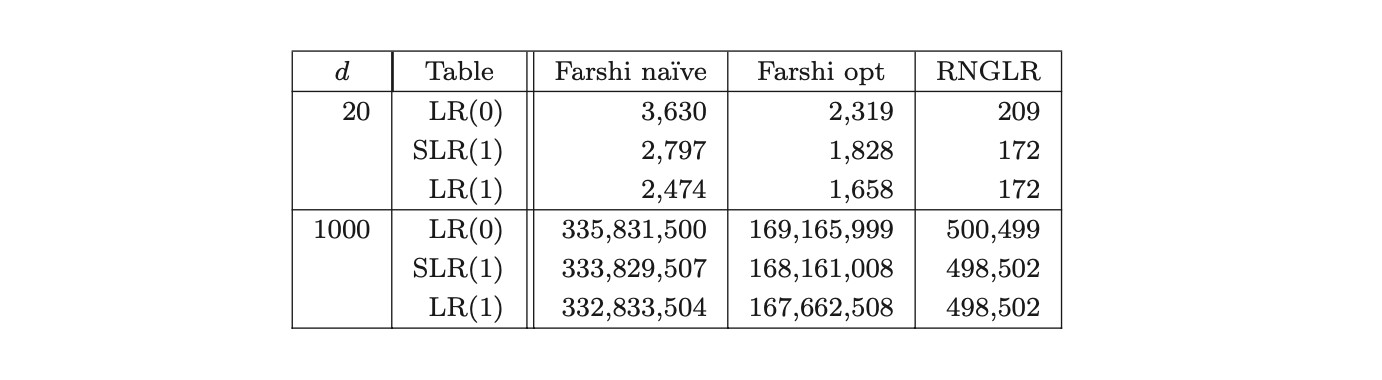Table 10.15: Edge visits performed parsing strings of the form \(b^d\) in Grammar 10.2.

10.6.3 The performance of Farshi’s algorithms

Although we expected the RNGLR algorithm to carry out significantly fewer edge visits than the either of the Farshi algorithms, it was surprising that the number of edge visits for the naive version of Farshi were so similar to the optimised version for ANSI-C and Pascal. To get a better understanding of the results, PAT was used to output diagnostics of the algorithm’s performance.

The optimised version of Farshi only triggers a saving when a new edge is added to an existing node in the current level of the GSS and the length of the reduction that is reapplied is greater than one. Therefore, if the majority of reductions performed have a length less than two, it is likely that the saving will not be as good as expected. To help reason about this behaviour PAT was used to create histograms of the number of times a reduction of length \(i\) was added to the set \(\mathcal{R}\) for the ANSI-C and Pascal experiments. The two histograms are shown in Figures 10.2 and 10.3. Their x-axis represents the reduction length and the y-axis the number of times a reduction was added to the set \(\mathcal{R}\).

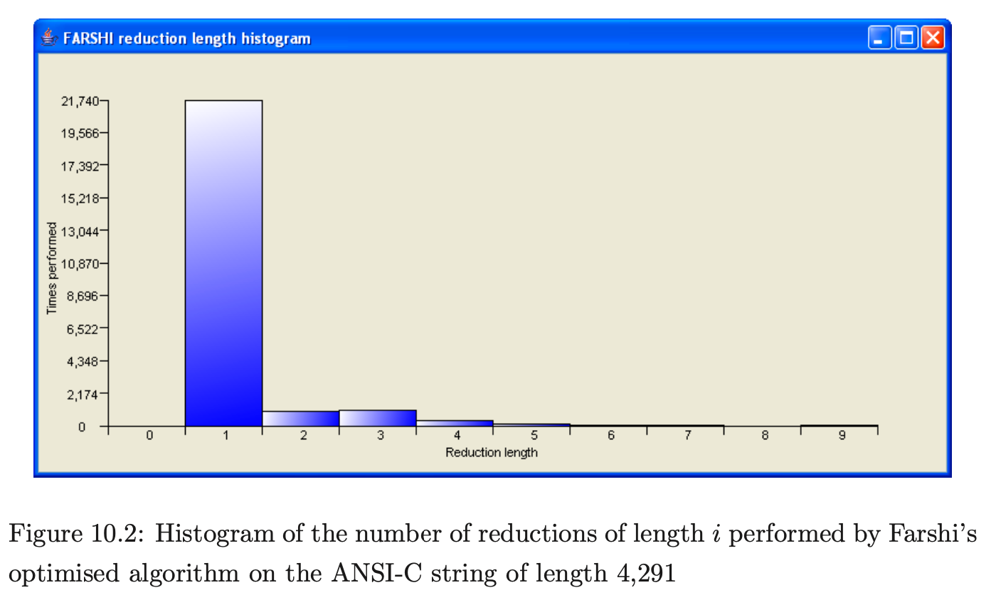
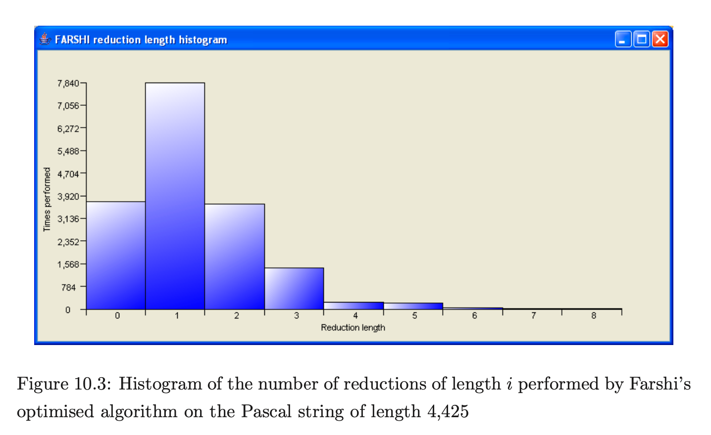
Both histograms show that the majority of reductions performed are of length one which explains why the results are so similar.

The number of edge visits performed parsing strings in Grammar 6.1 differ greatly between the two Farshi algorithms. By counting the number of edge visits contributed by reductions of a certain length, we can see where the optimised version of Farshi is making a saving. We used PAT to generate the histograms in Figures 10.4 and 10.5 that show the number of edge visits performed for reductions of length in Grammar 6.1. The x-axis represents the different reduction lengths and the y-axis the number of edge visits performed.

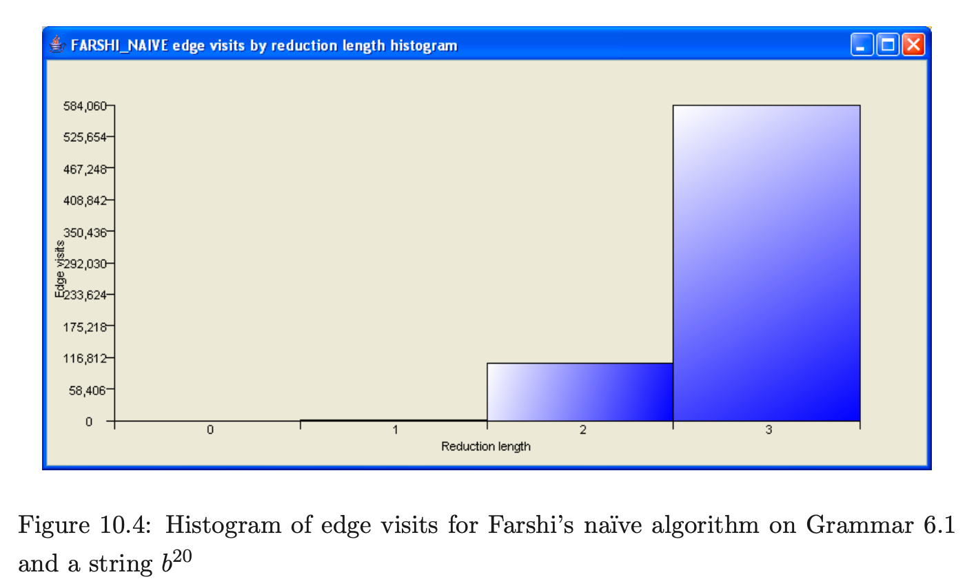
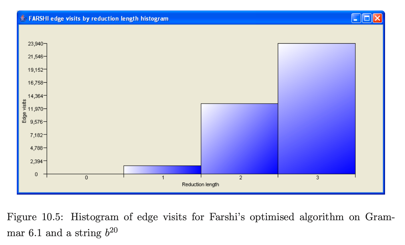
For Grammar 6.1 there is a difference of 653,620 edge visits because there are few reductions of length one and none of length zero and the other reductions have triggered a significant saving.

In this section we have shown that the RNGLR algorithm is the most efficient of the algorithms compared. However, its worst case complexity is still \(O(n^{k+1})\) whereas other algorithms that effectively modify the grammar into 2-form claim cubic worst case complexity. The BRNGLR algorithm presented in Chapter 6 is one such technique. Next we compare the efficiency between the RNGLR and BRNGLR algorithms.

10.7 The performance of the BRNGLR algorithm

This section compares the performance of the BRNGLR and RNGLR parsing algorithms discussed in Chapters 5 and 6 respectively. We present the results of parses for our three programming languages and Grammar 6.1. We begin by discussing the results of the latter experiment which generates worst case behaviour for the BRNGLR algorithm and supra cubic behaviour for the RNGLR algorithm.

10.7.1 GSS construction

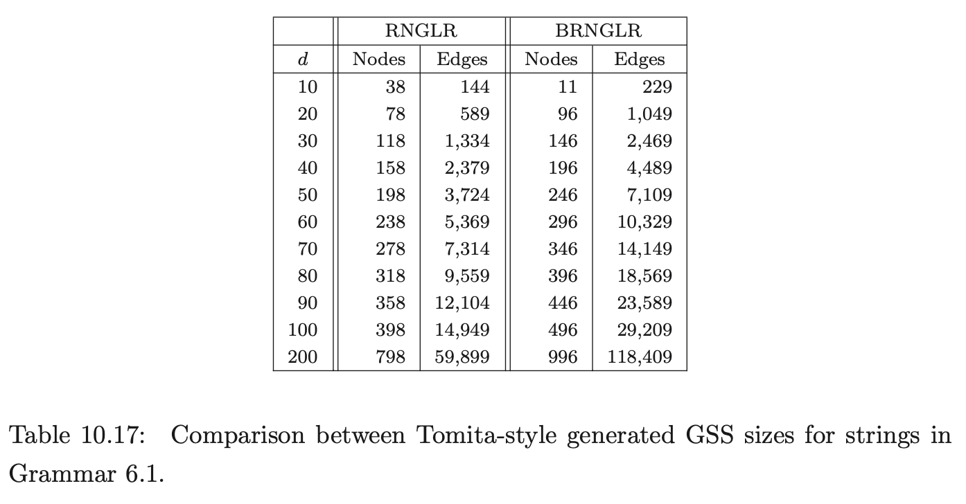
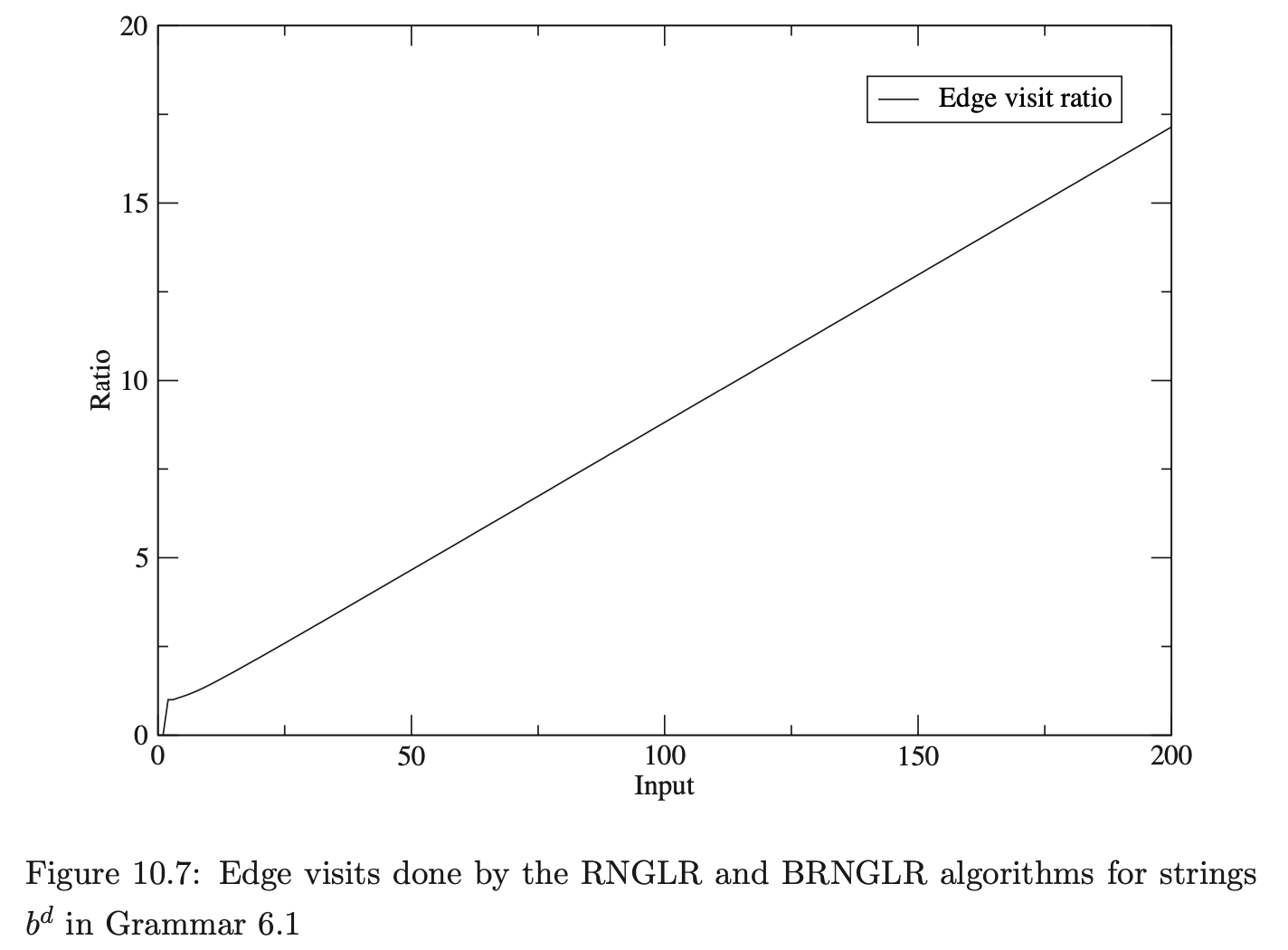
The number of edge visits performed by each algorithm are shown in Table 10.16. Recall that, for both algorithms, the creation of an edge is not counted as an edge visit and the first edge in a reduction path is not visited because of the way pending reductions are stored in the set \(\mathcal{R}\). As it is sometimes difficult to distinguish between data that has been generated by a cubic, quartic or other polynomial function, the edge visit ratio, which we expect to be linear, is also presented. 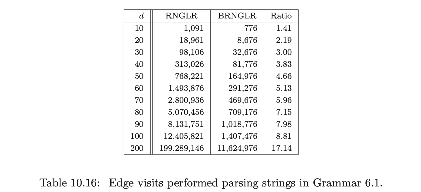Because of the regularity of Grammar 6.1 we can compute by hand, the number of edge visits made by the BRNGLR algorithm on \(b^{d}\). For \(d\geq 3\), the number is

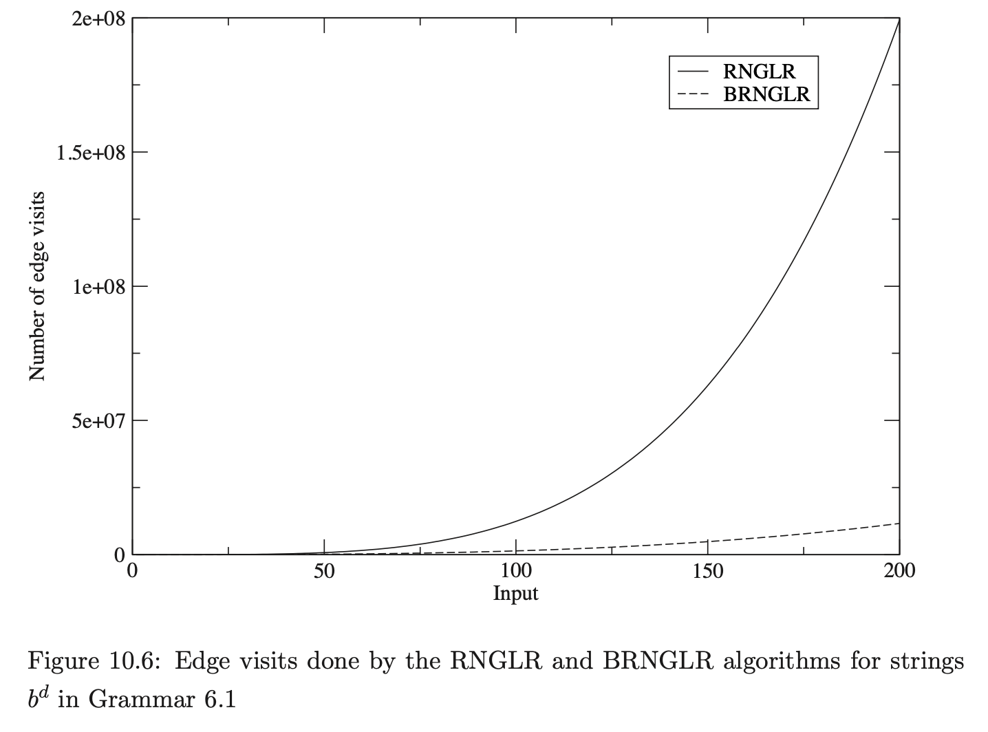
The experimental results do indeed fit this formula. Table 10.16 only shows a sample of the data gathered. In fact the algorithm was run for all strings \(b^{d}\) for lengths from 1 to 200. This data was exported to Microsoft Excel and used to generate two polynomial trend-lines for the data gathered for both algorithms. Using the RNGLR trend-line we have generated the following formula for the number of RNGLR edge visits, which matches the 201 data points exactly. As expected it is a quartic polynomial.

It is worth noting here that the BRNGLR algorithm implementation parsed \(b^{1000}\) in less than 20 minutes, while the ‘GLR’ version of Bison could not parse \(b^{20}\).

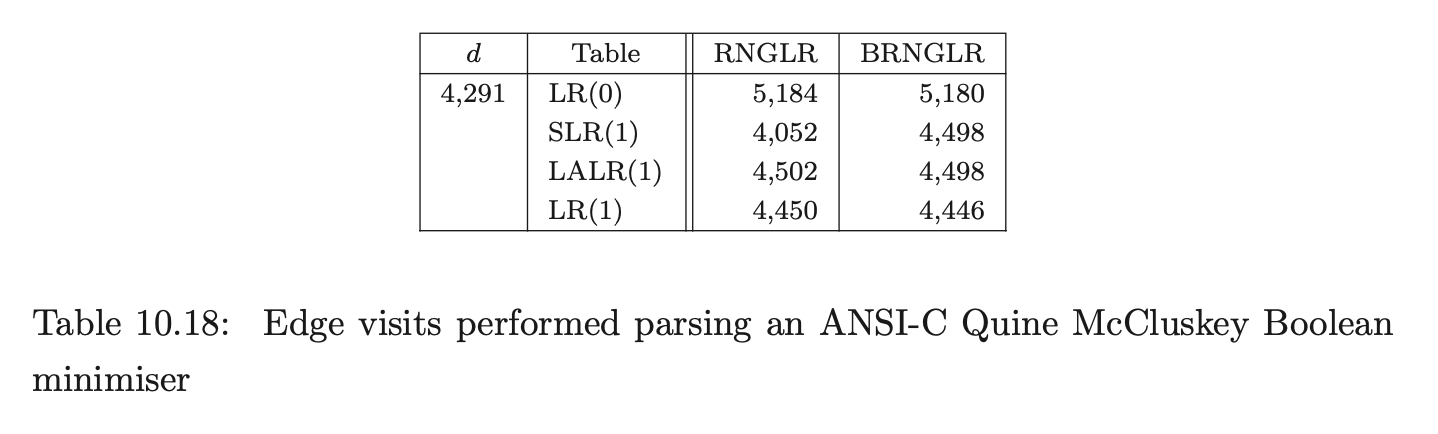
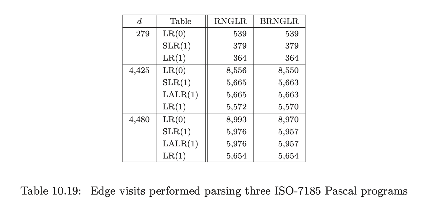
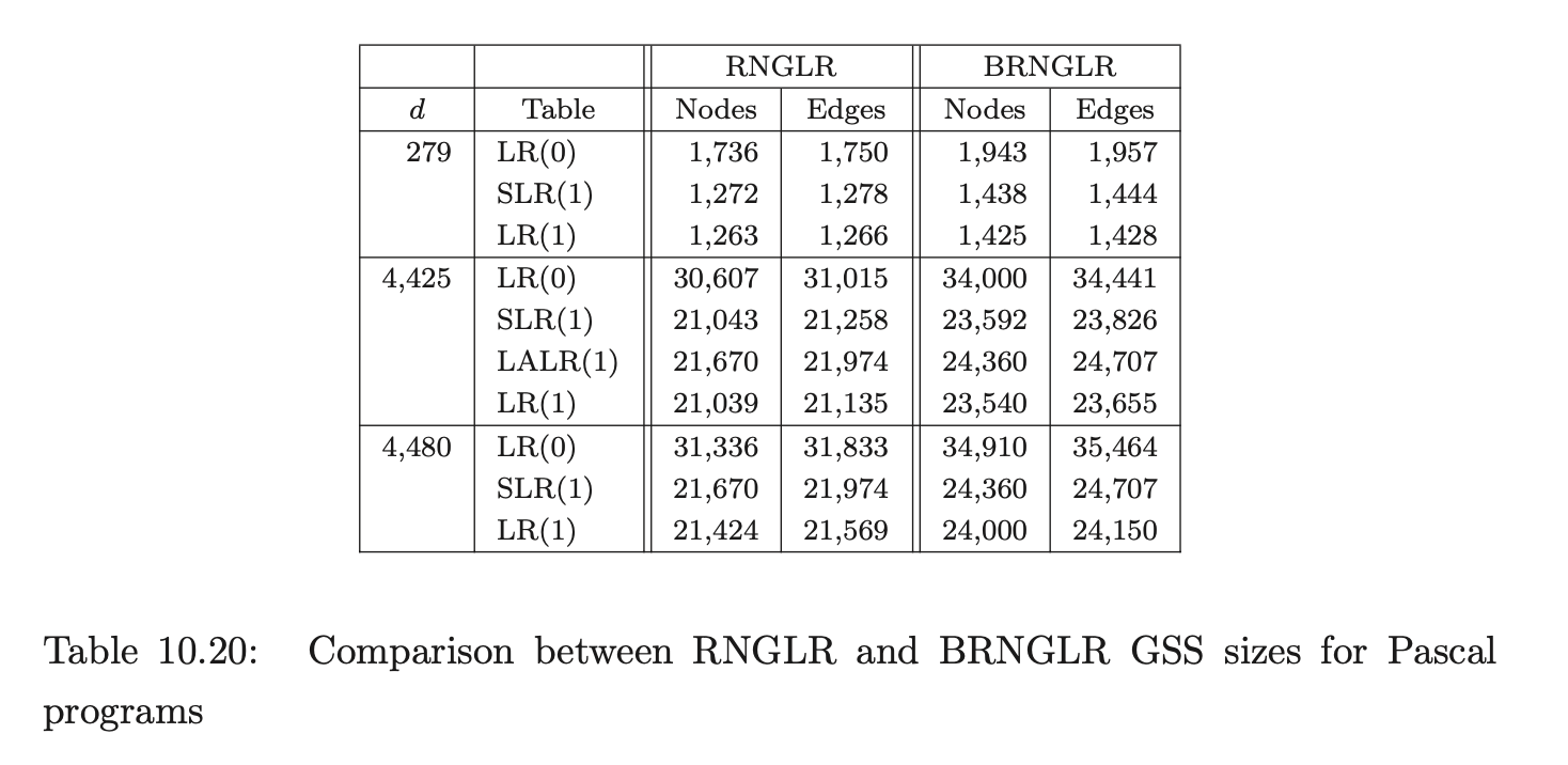
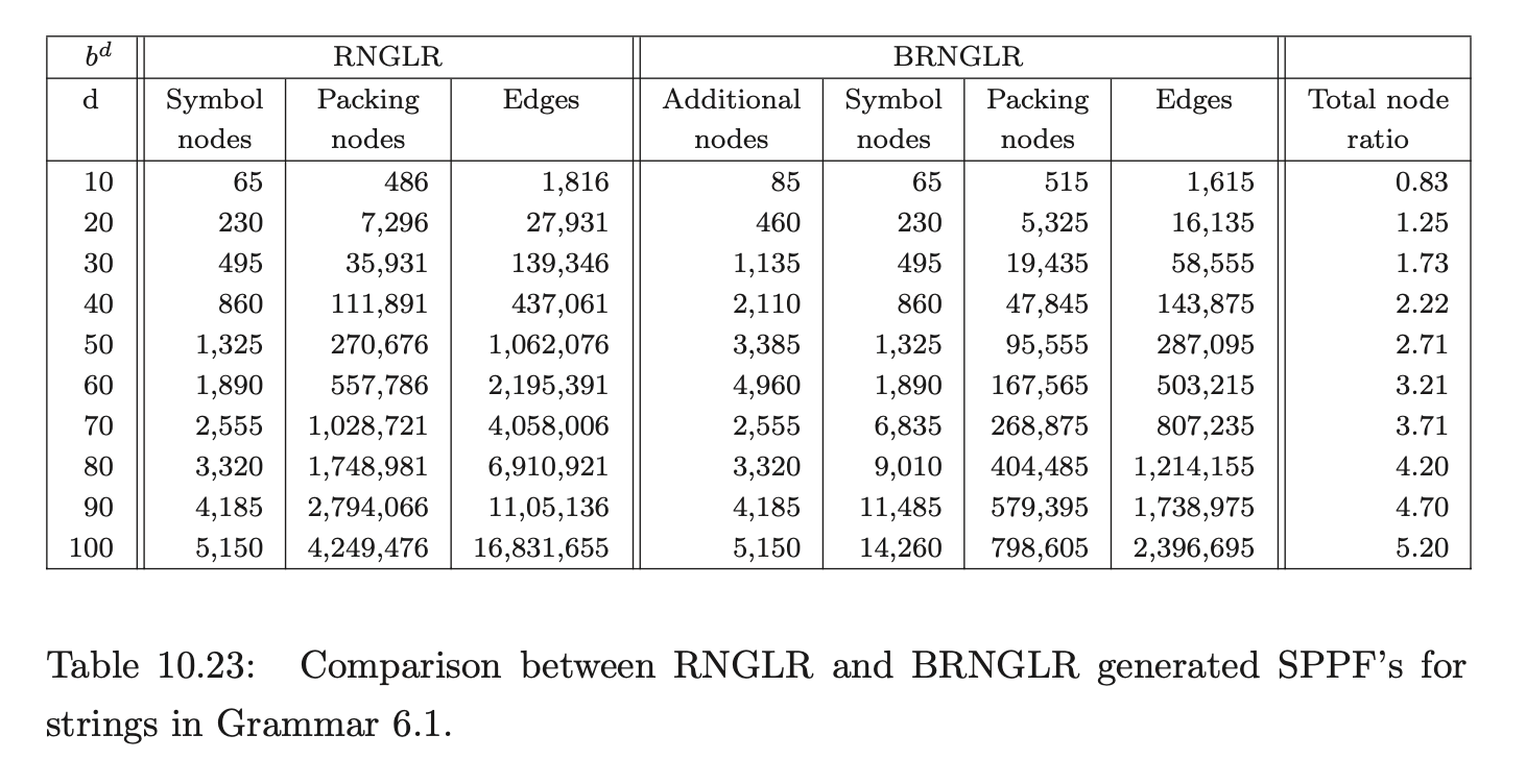
Whilst the BRNGLR algorithm improves the worst case performance, it is of course important that this improvement is not at the expense of average case behaviour. To demonstrate that the BRNGLR algorithm is not less practical than the RNGLR algorithm we have run both algorithms with all three of our programming language grammars. We expect a similar number of edge visits to be performed for both algorithms.

10.7.2 SPPF construction

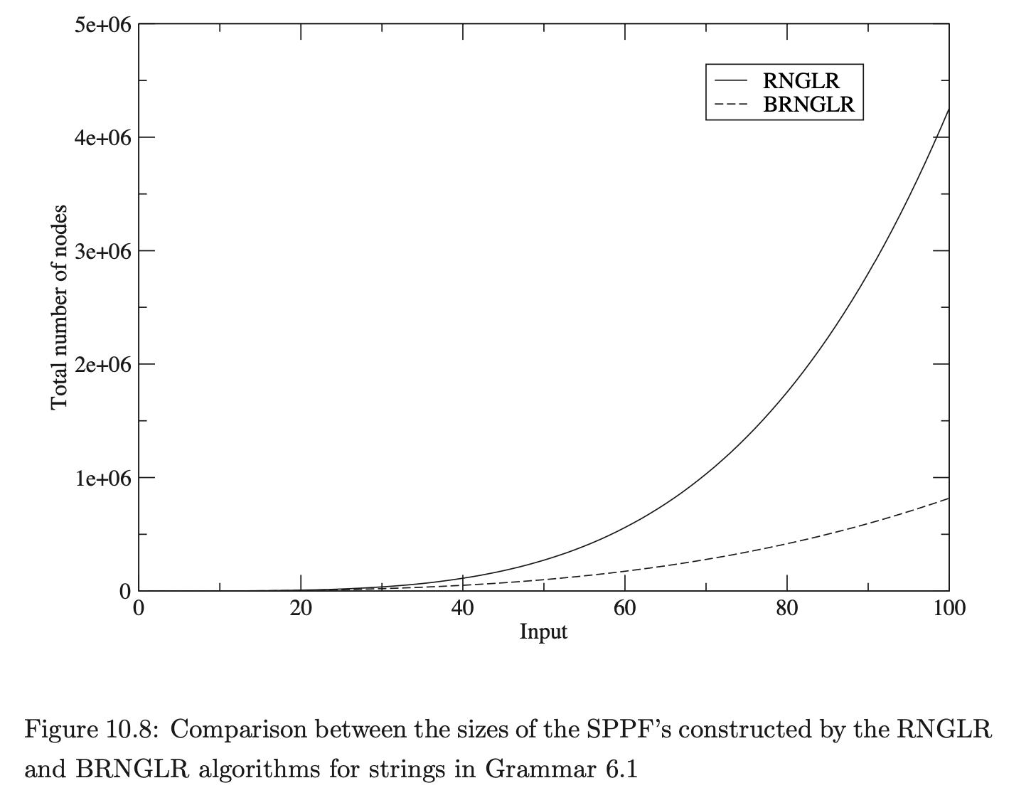
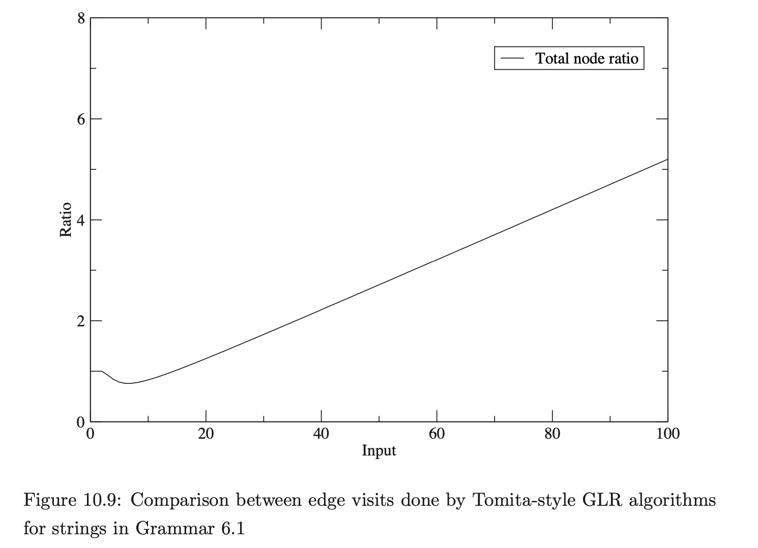
As we discussed in Section 6.6, the parser version of the BRNGLR algorithm must retain the cubic order of the underlying recogniser. To illustrate this, data was also collected about the space required for the SPPF’s of Grammar 6.1. The number of symbol nodes, additional nodes, packing nodes and edges in the SPPF were recorded. We expect the size of the SPPF generated for Grammar 6.1 by the RNGLR algorithm to be quartic and cubic for the BRNGLR algorithm. To highlight the difference between the two algorithms, the total node ratio, which we expect to be linear, has also been calculated.

The BRNGLR algorithm generates SPPF’s an order of magnitude smaller than the RNGLR algorithm for strings in the language of Grammar 6.1. Microsoft Excel was used to generate the following charts of the data.

The Excel generated equation for the number of packing nodes created by the RNGLR algorithm is

The Microsoft Excel generated equation for the number of packing nodes created by the RNGLR algorithm is

Because of the irregular way packing nodes are created for \(d<4\), approximation errors occur in the Excel generated charts. By replacing the decimal coefficients with more precise fractions, the correct equation for the number of packing nodes in the RNGLR SPPF can be determined. For \(d>3\) the equation is

Similarly the correct equation for the number of packing nodes in the SPPF generated by the BRNGLR algorithm, for \(d>3\), is

To show that the average case performance for the generation of SPPF’s is not compromised, SPPF’s were also generated for the ANSI-C, Pascal and Cobol programs previously described.

The results presented in this section complement the theoretical analysis of the BRNGLR algorithm. In the next section we compare BRNGLR with Earley’s recognition algorithm that is known to also have cubic worst case complexity.

10.8 The performance of Earley algorithm

We discussed Earley’s algorithm in Chapter 8. We have implemented his recognition algorithm within PAT and generated statistical data on its performance. We compare the size of the Earley sets with the size of the GSS constructed by the RNGLR and BRNGLR algorithm using an RNLR(1) parse table (except for the Cobol parse which uses an RNSLR(1) table) and the number of symbol comparisons required to construct the Earley sets with the number of edge visits performed by the RNGLR and BRNGLR algorithms.

Earley’s algorithm is known to be cubic in the worst case, quadratic for unambiguous grammars and linear on the class of linear bounded grammars [1]. We begin by comparing the performance of the three algorithms during the parse of strings \(b^{d}\) for Grammar 6.1. Recall that this grammar triggers supra cubic behaviour for the RNGLR algorithm and cubic behaviour for the BRNGLR algorithm. Since it is ambiguous we expect Earley’s algorithm to display at least quadratic behaviour.

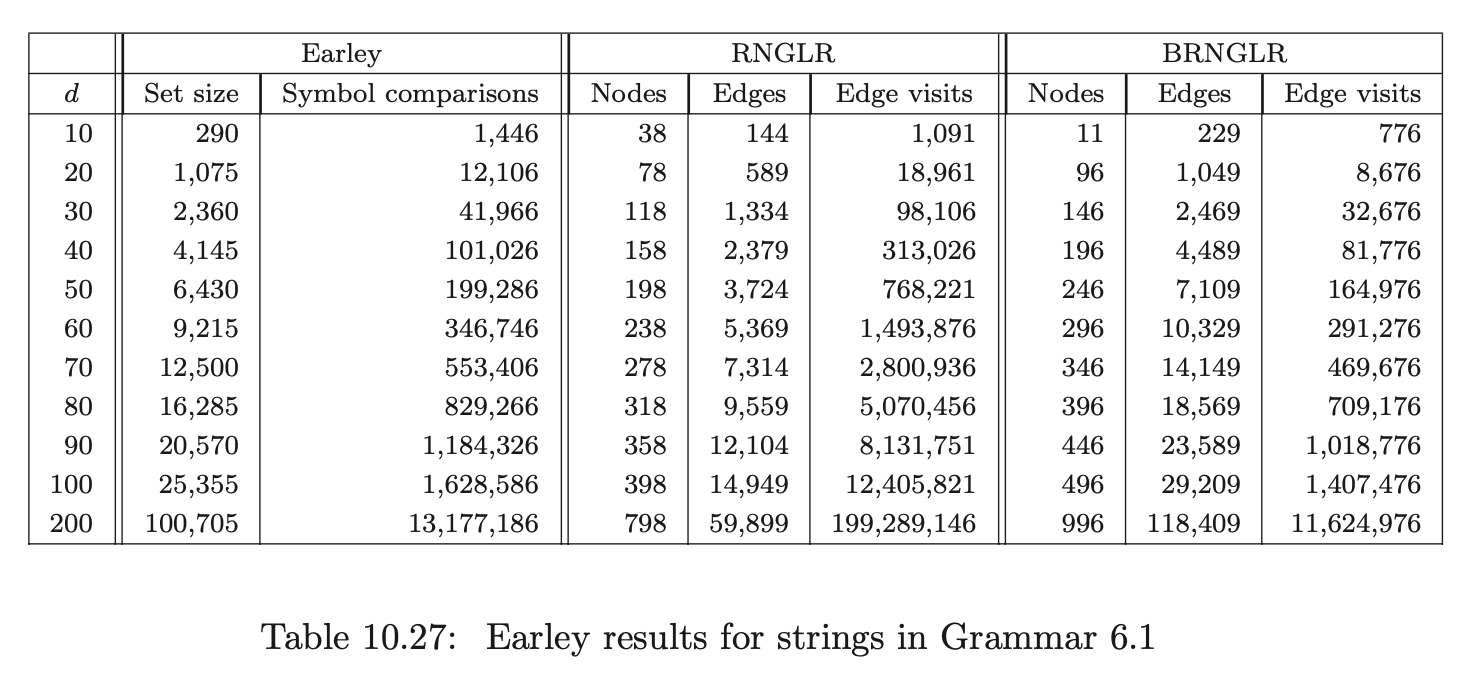As expected Earley’s algorithm performs an order of magnitude fewer symbol comparisons than the RNGLR algorithm’s edge visits. It compares well to the BRNGLR algorithm. Next we present the results of the parses for our three programming languages.

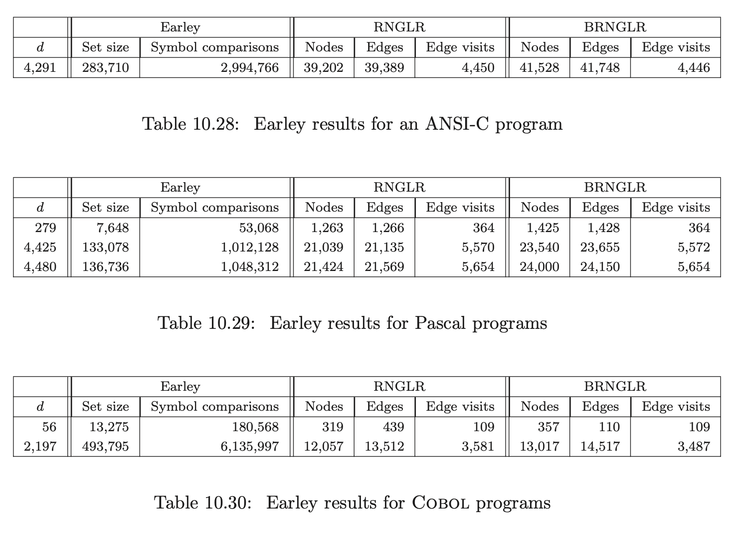
Both the RNGLR and the BRNGLR algorithms compare very well to Earley’s algorithm for all of the above experiments.

All of the algorithms that we have compared so far have focused on efficiently performing depth-first searches for non-deterministic sentences. In Chapter 7 we presented the RIGLR algorithm which attempts to improve the parsers’ efficiency by restricting the amount of stack activity. The next section presents the results collected for the parses of the RIGLR algorithm on our four grammars. We compare the performance of the RIGLR algorithm to the RNGLR and BRNGLR algorithms.

10.9 The performance of the RIGLR algorithm

The asymptotic and typical actual performance of the RIGLR algorithm is demonstrated by comparing it to the RNGLR and BRNGLR algorithms. We use the grammars for ANSI-C, Pascal and Cobol as well as Grammar 6.1. We begin this section by discussing the size of the RIA’s and RCA’s constructed by GTB and used by PAT for the experiments.

10.9.1 The size of RIA and RCA

Part of the speed up of the RIGLR algorithm over the RNGLR algorithm is obtained by effectively unrolling the grammar. In a way this is essentially a back substitution of alternates for instances of non-terminals on the right hand sides of the grammar rules. Of course, in the case of recursive non-terminals the back substitution process does not terminate, which is why such instances are terminalised before the process begins.

We terminalised and then built the RIA’s and RCA’s for ANSI-C, Pascal, Cobol and Grammar 6.1 described above. In each case the grammars were terminalised so that all but non-hidden left recursion was removed before constructing the RIA’s. Table 10.31 shows the number of terminalised non-terminals, the number of instances of these terminalised non-terminals in the grammar, the number of symbol labelled transitions in RCA(\(\Gamma\)) and the number of reduction labelled transitions in RCA(\(\Gamma\)). (It is a property of RCA(\(\Gamma\)) that the number of states is equal to the number of symbol labelled transitions + the number of terminalised nonterminal instances + 1.)

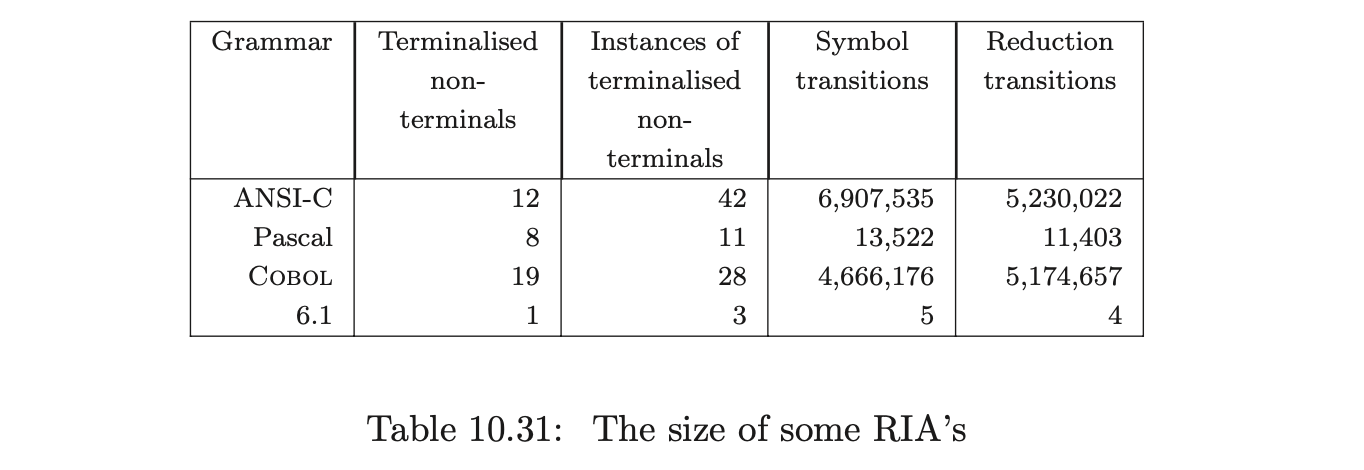
The size of some RIA’sThe size of the RCA’s for ANSI-C and Cobol are impractically large. The potential explosion in automaton size is not of itself surprising: we know it is possible to generate an LR(0) automaton which is exponential in the size of the grammar. The point is that the examples here are not artificial. Some properties of grammars that cause this kind of explosion to occur are discussed in detail in [13]. The construction of these automata is made difficult because of their size. In particular, the approach of constructing the RCA by first constructing the IRIA’s and RIA, as presented in Chapter 7, can be particularly expensive. A more efficient construction approach that involves performing some aspects of the subset construction ‘on-the-fly’ is presented in [JSE04a].

Ultimately the way to control the explosion in the size of RCA is to introduce more non-terminal terminalisations. In order for the RIGLR algorithm to be correct, it is necessary to terminalise the grammar so that no self embedding exists, but the process is still correct if further terminalisations are applied.

Although this will reduce the size of parser for some grammars, it comes at the cost of introducing more recursive calls when the parser is run and hence the (practical but not asymptotic) run time performance and space requirements of the parser will be increased. Thus there is an engineering tradeoff to be made between the size of the parser and its performance.

10.9.2 Asymptotic behaviour

To measure the run-time performance of the RNGLR and BRNGLR algorithms we count the number of edge visits performed for the application of reductions, in the way described in Section 10.6. For the space required we count the number of state nodes and edges in the GSS as well as the maximum size of the set \(\mathcal{R}\). For the RIGLR algorithm we measure the run-time performance by counting the number of RCA edge visits performed during the execution of pop actions and the space by the total number of elements added to the set \(U_{i}\).

Figure 10.11 and Table 10.33 present the number of edge visits performed by RNGLR, BRNGLR and RIGLR algorithms for parses of the string \(b^{d}\) in Grammar 6.1. The RIGLR and BRNGLR algorithms display cubic time complexity whereas the RNGLR algorithm displays quartic time complexity.

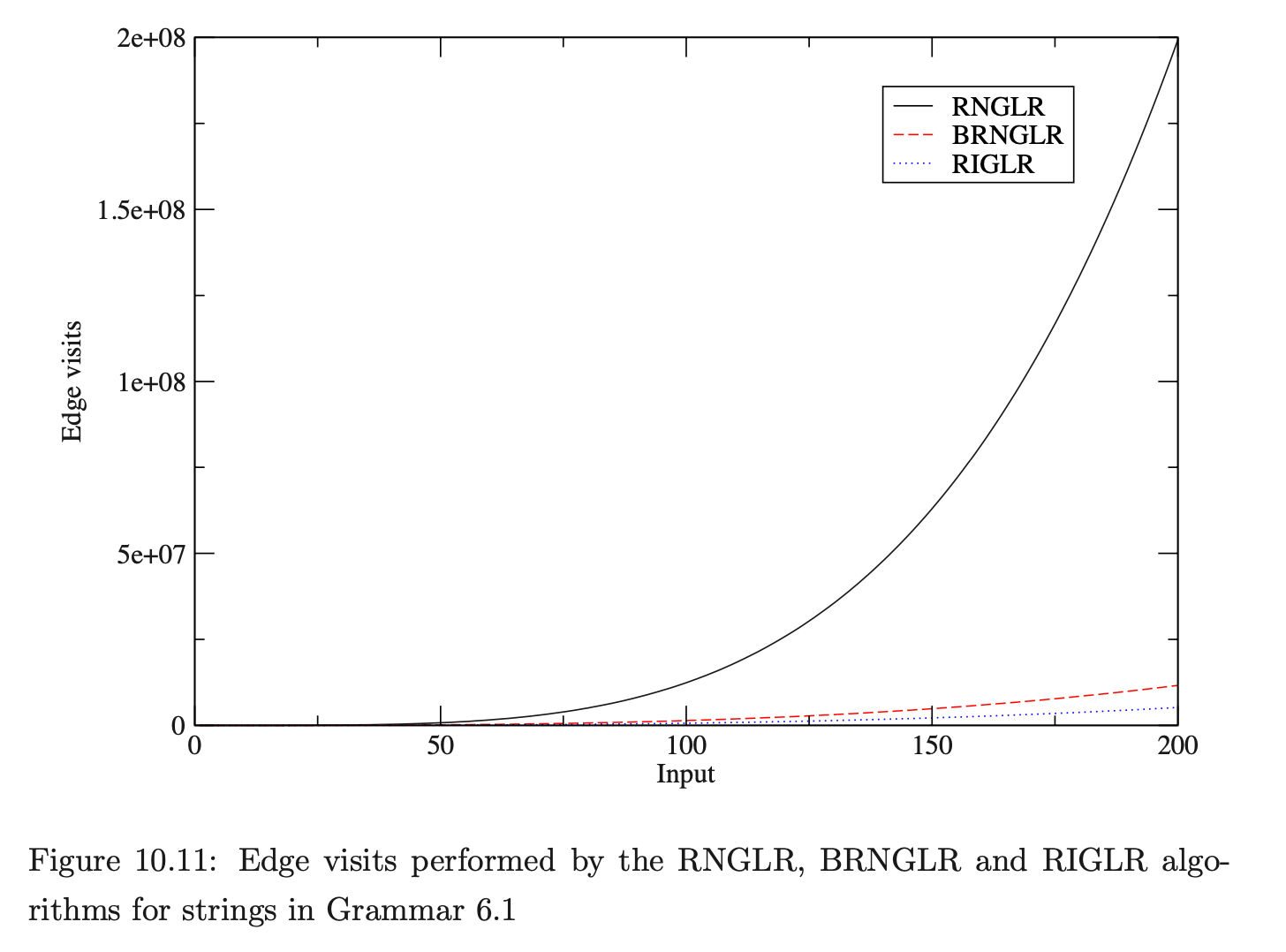
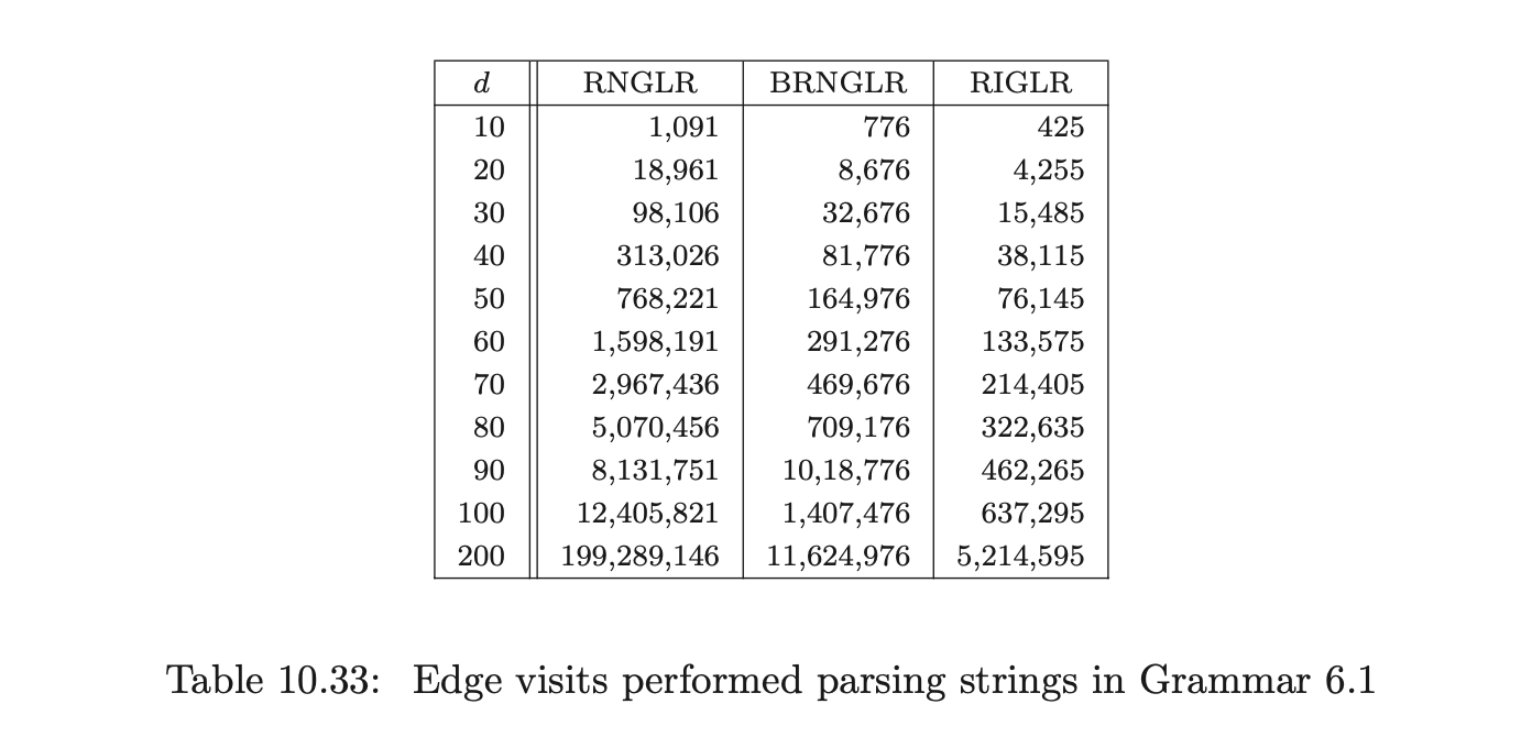
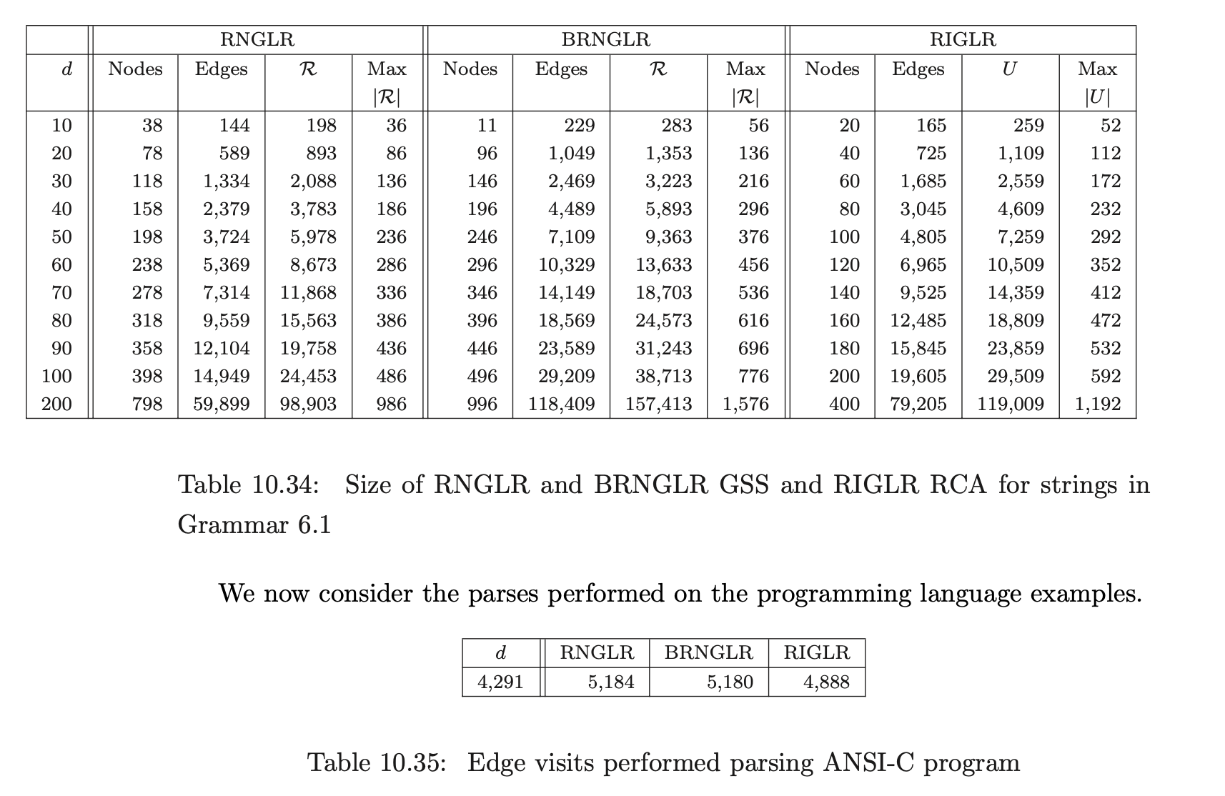
The size of the structures constructed during the parses by the separate algorithms indicate that the RIGLR algorithm achieves an order of magnitude reduction of space compared to the RNGLR and BRNGLR algorithms. The examples also show that the number of edge visits performed by the RIGLR algorithm compare well to the results of the RNGLR and BRNGLR algorithms.