4. Generalised LR parsing¶

As we have already discussed in earlier chapters, context-free grammars were developed by Noam Chomsky in the 1950’s in an attempt to capture the key properties of human languages. Computer scientists took advantage of their declarative structure and used them to define the syntax of programming languages. Many parsing algorithms capable of parsing all context-free grammars were developed, but their poor worst case performance often made then impractical. As a result more efficient parsing algorithms which worked on a subclass of the context-free grammars were developed.

The efficiency of the contemporary generalised parsing techniques (CYK, Earley, etc.) were disappointing when compared to Knuth’s deterministic LR parsing algorithm. Its popularity had soared, but the class of grammars it accepted was too restrictive for the practical applications that interested Tomita - natural language processing. In 1985, he developed the GLR parsing algorithm by extending the LR algorithm to work on non-LR grammars.

This chapter presents Tomita’s GLR recognition and parsing algorithms [Tom86, Tom91]. Although these algorithms work for a larger class of grammars than the LR parsers they cannot correctly parse all context-free grammars. We discuss the modification due to Farshi [NF91], that extends Tomita’s recognition algorithm to work for all context-free grammars and then discuss Rekers’ [Rek92] parser extension.

4.1 Using the LR algorithm to parse all context-free grammars¶

In Chapter 2 we described the standard LR parsing algorithm. LR parsers are extremely efficient, but are restricted by the class of grammars they accept. Although they work for a useful subset of the context-free grammars, they cannot cope with non-determinism.

A naive approach to dealing with non-determinism in an LR parser is to duplicatea stack when a conflict in the parse table is encountered. An approach presented in [12] uses a stack list to represent the different stacks of a non-deterministic parse. Each stack in the stack list is controlled by a separate LR parsing process that works in the same way as the standard LR algorithm. However, each process essentially works in parallel by synchronising on the shift actions.

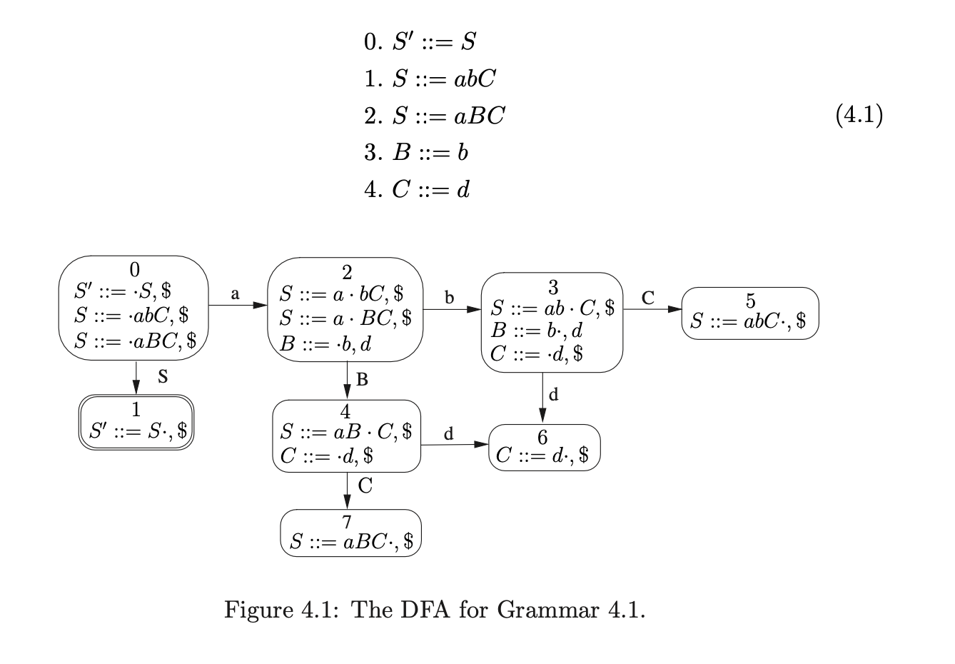
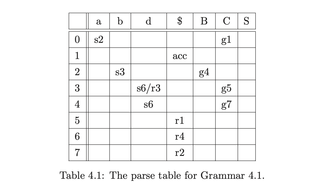
Each stack in the stack list is represented by a graph, where the nodes are labelled with a state number and the edges are labelled with the symbol parsed. The right-most nodes are the tops of each stack. For example, consider the parse of the string $abd$ for the ambiguous Grammar 4.1 and the DFA in Figure 4.1. The associated LR(1) parse table, with conflicts, is shown in Table 4.1.

We begin the parse by creating the start node, $v_{0}$, of the stack list, labelled by the start state of the DFA. We read the first input symbol, $a$, and then perform the shift from state $0$ to state $2$. We create a new node, $v_{1}$ in the stack list, labelled $2$, and add an edge, labelled $a$ back to $v_{0}$.

We then proceed to read the next input symbol, $b$, and create the node, $v_{2}$, labelled $3$ with an edge back to $v_{1}$. At this point we are in state $3$ of the DFA which contains a shift/reduce conflict. Since we do not know which action to perform, we duplicate the stack and perform both actions. We synchronise the stack list on shift actions, so we perform the reduce $B::=b$ on the bottom stack first. This involves popping the node $v_{5}$ off the stack and adding a new node $v_{6}$, labelled $4$, with an edge labelled $B$ back to $v_{4}$.

We then read the next input symbol, $d$, and perform the synchronised shift action, $s6$, for both stacks. We create the new nodes $v_{7}$ and $v_{8}$, with edges labelled $d$, back to $v_{2}$ and $v_{6}$ respectively. Since there is a reduce on rule $C::=d$ from both states at the top of the stack list we can perform both to get the new stack list shown below.

From state 5 there is a reduce on $S::=abC$ so we pop the top 3 nodes off the first stack and create the new node, $v_{11}$, labelled 1, with an edge from $v_{11}$ to $v_{0}$.

From state 7 there is a reduction on rule $S::=aBC$, so we pop the top 3 nodes off the second stack as well and create the new node, $v_{12}$ as shown below. Since all the input has been consumed and $v_{10}$ and $v_{11}$, which are labelled by the accept state of the DFA, are at the top of the stack list the parse has succeeded.

Using a stack list to follow all parses of an ambiguous sentence can be very inefficient. If a state can be reached in several different ways, because of non-determinism, then there will be several duplicate stacks. Unfortunately, this can cause the number of stacks created to grow exponentially. In addition to this, because the stacks do not share any information with each other, if the tops of several stacks contain the same state then they continue to parse the remaining input in the same way until the duplicate states are popped off each stack.

Such redundant actions can be prevented with the use of a slightly modified structure called a Tree Structured Stack (TSS) [16]. When the tops of two or more stacks contain the same state, a single state is shared between each stack. This prevents duplicate parses of the same input being done.

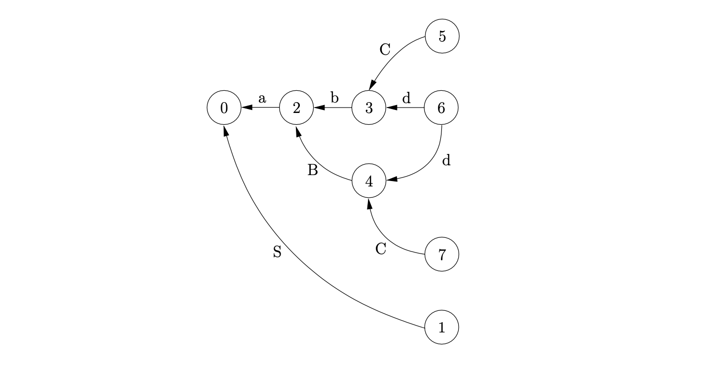
For example, consider the parse of the string $abd$ shown above. After duplicating the stack and performing the first reduction the next action is a shift on $d$. Since both stacks reach state 6 on the shift we can merge the nodes $v_{8}$ and $v_{9}$ to combine the stack list into a TSS. Although this approach significantly improves the efficiency of the algorithm, it is still far from ideal - the number of stacks created can still grow exponentially. In both approaches discussed above, when a conflict in the parse table is encountered the entire stack is duplicated. However, it is often the case that separate stacks have the same nodes towards the bottom of the stack (the leaves of the TSS). Instead of duplicating a stack when a non-deterministic point in the parse is reached, the space required can be reduced by only splitting the necessary part of the stack. The resulting structure is called a Graph Structured Stack (GSS) [16]. The GSS constructed for the parse of the string $abd$ is shown below.

The next section presents Tomita’s Generalised LR (GLR) algorithm that extends the standard LR parser by constructing a GSS during a parse.

4.2 Tomita’s Generalised LR parsing algorithm¶

In [16], Tomita presents five separate GLR algorithms which we shall refer to as Algorithms 0-4. The first four algorithms are recognisers and the fifth algorithm is the extension of Algorithm 3 to a parser. Algorithm 0 is defined to work for LR(1) grammars and is used to introduce the construction of the GSS. Algorithm 1 extends Algorithm 0 to work for non-LR(1) grammars without $\epsilon$-rules. Algorithm 2 introduces a complex approach to deal with $\epsilon$-rules and forms the basis of Algorithm 3 - the full version of the recognition algorithm. Algorithm 4 is the parser version of the GLR algorithm which constructs a shared packed parse forest representation of parse trees.

This section introduces Tomita’s recognition Algorithms 1 and 2. We begin by defining the central data structure that underpins all of Tomita’s algorithms - the GSS. We demonstrate the construction of the GSS for both algorithms and highlight some of the problems associated with each of the approaches. Algorithms 3 and 4 are discussed in Section 4.4.

4.2.1 Graph structured stacks¶

A Graph Structured Stack (GSS) is the central data structure that underpins all of Tomita’s GLR algorithms. An instance of a GSS is related to a specific grammar $\Gamma$ and input string $a_{1}\dots a_{n}$. It is defined as a directed acyclic graph, containing two types of node: state nodes, labelled by the state numbers of the DFA for $\Gamma$ and symbol nodes, labelled by $\Gamma$’s grammar symbols.

The state nodes are grouped together into $n+1$ disjoint sets called levels. The GSS is constructed one level at a time. First all possible reductions are performed for the state nodes in the current level (the frontier), and then the next level is created as a result of applying shift actions. The first level is initialised with a state node labelled by the $DFA's$ start state.

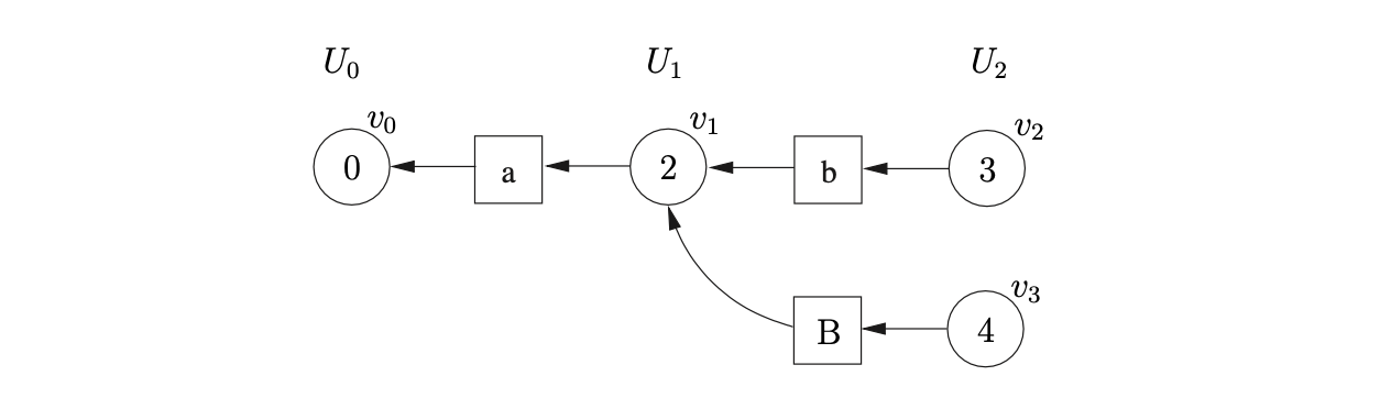
We represent a GSS graphically by drawing the state nodes as circular nodes and the symbol nodes are square nodes. To separate each of the levels we draw the state nodes of a given level in a single column labelled $U_{i}$, where $0\leq i\leq n$. The GSS is drawn from left to right, with the rightmost nodes representing the tops of each of the stacks.

4.2.2 Example - constructing a GSS¶

We shall describe how a GSS is constructed during the parse of a string $abc$ with Grammar 4.1, whose DFA shown in Figure 4.1 and the associated parse table in Table 4.1. We shall refer to the parse table as $\mathcal{T}$.

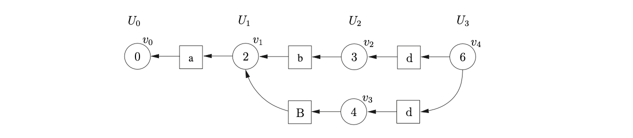
The GSS is initialised with the state node, $v_{0}$, in level $U_{0}$. For each new state node constructed in the GSS we check to see what actions are applicable. We begin the parse by finding the shift action s2 in $\mathcal{T}(0,a)$. This triggers the creation of the next level, $U_{1}$ for which we create the new node, $v_{1}$, labelled 2. We create a new symbol node, labelled $a$, and make it the successor of $v_{1}$ and the predecessor of $v_{0}$.

We process $v_{1}$ and find the shift action s3 in $\mathcal{T}(2,b)$. We construct the new node, $v_{2}$ labelled 3 and add it to level $U_{2}$. We read the $b$ from the input string, construct the new symbol node labelled $b$ and make it the successor of $v_{2}$ and the predecessor of $v_{1}$.

Next we process $v_{3}$. In $\mathcal{T}(3,c)$ there is a shift/reduce conflict, s6/r3. Since the construction of the GSS is synchronised on the shift actions, we queue the shift, and continue by performing the reduction by rule 3, $B::=b$. Unlike the standard LR parser that removes states from the parse stack when a reduction is performed, a GLR algorithm does not remove nodes from the GSS[1]. Instead of popping nodes off the stack, we perform a traversal of all reduction paths of length 2, from node $v_{2}$, to find the target nodes of the reduction. In this case there is only one path, which leads to node $v_{1}$. We find the goto action, g4 $\in\mathcal{T}(2,B)$, and create the new state node, $v_{3}$, labelled 4 in the current level $U_{2}$. We then create the symbol node labelled $B$ and make it the successor of $v_{3}$ and the predecessor of $v_{1}$.

The only action associated with the newly created node, $v_{3}$, is the shift s6. Since we have processed all nodes in $U_{2}$ and performed all possible reductions the current level is complete. So next we construct level $U_{3}$ by performing the shift actions from $v_{2}$ and $v_{3}$. We create the new node, $v_{4}$, labelled 6, in $U_{3}$ and two new symbol nodes labelled $d$. We then add two paths of length 2 from $v_{4}$, one going to $v_{2}$ and the other going to $v_{3}$.

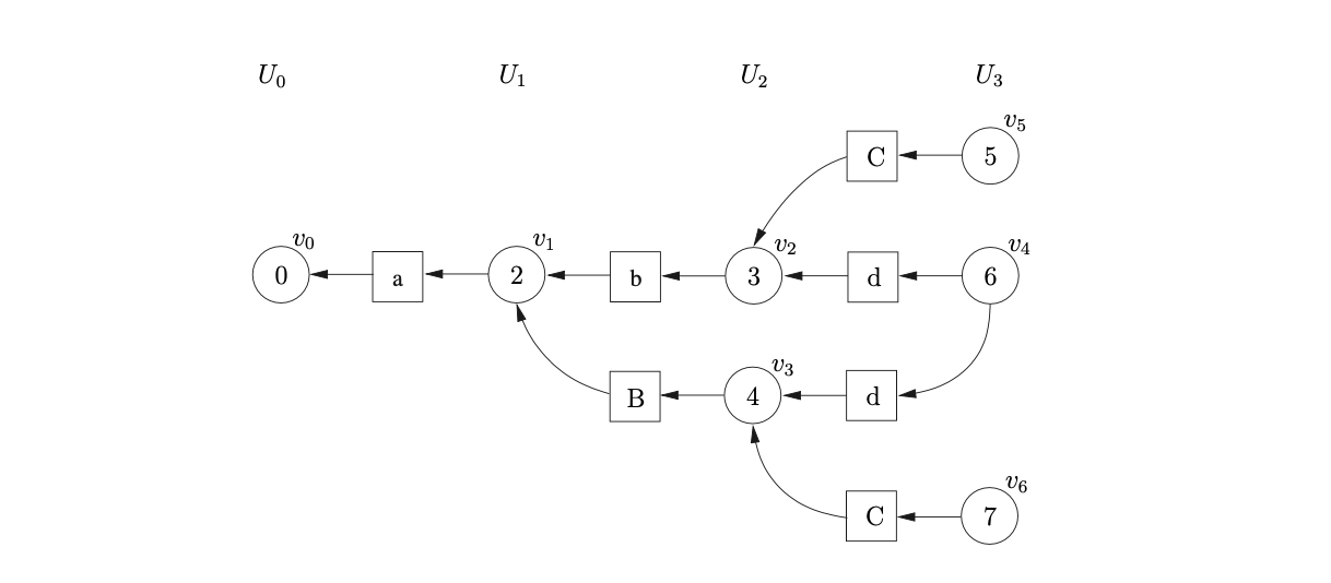
At this point we have consumed all the input symbols and are left with the lookahead symbol $\$$. We process $v_{4}$ and find the reduce action r4 $\in\mathcal{T}(6,\$)$. Since the right hand side of rule 4 contains one symbol we trace back paths of length 2 from $v_{4}$. In this case two possible paths exist; one reaching $v_{2}$ and the other $v_{3}$. We create two new nodes, $v_{5}$ and $v_{6}$, labelled with the goto states found in $\mathcal{T}(3,C)$ and $\mathcal{T}(4,C)$ respectively. We create two new symbol nodes, both labelled $C$ and use them to create a path between $v_{5}$ and $v_{2}$ and $v_{6}$ and $v_{3}$. Processing both nodes $v_{5}$ and $v_{6}$ we see that the reduction r1 is applicable. The right hand side of rule 1 consists of 3 symbols, so we need to find the nodes at the end of the paths of length 6. Both reduction paths reach $v_{0}$ and since the associated goto action is the same for both reductions we create one new node, $v_{7}$, labelled 1 in the current level. Only one symbol node labelled $S$ is required, with a path from $v_{7}$ to $v_{0}$.

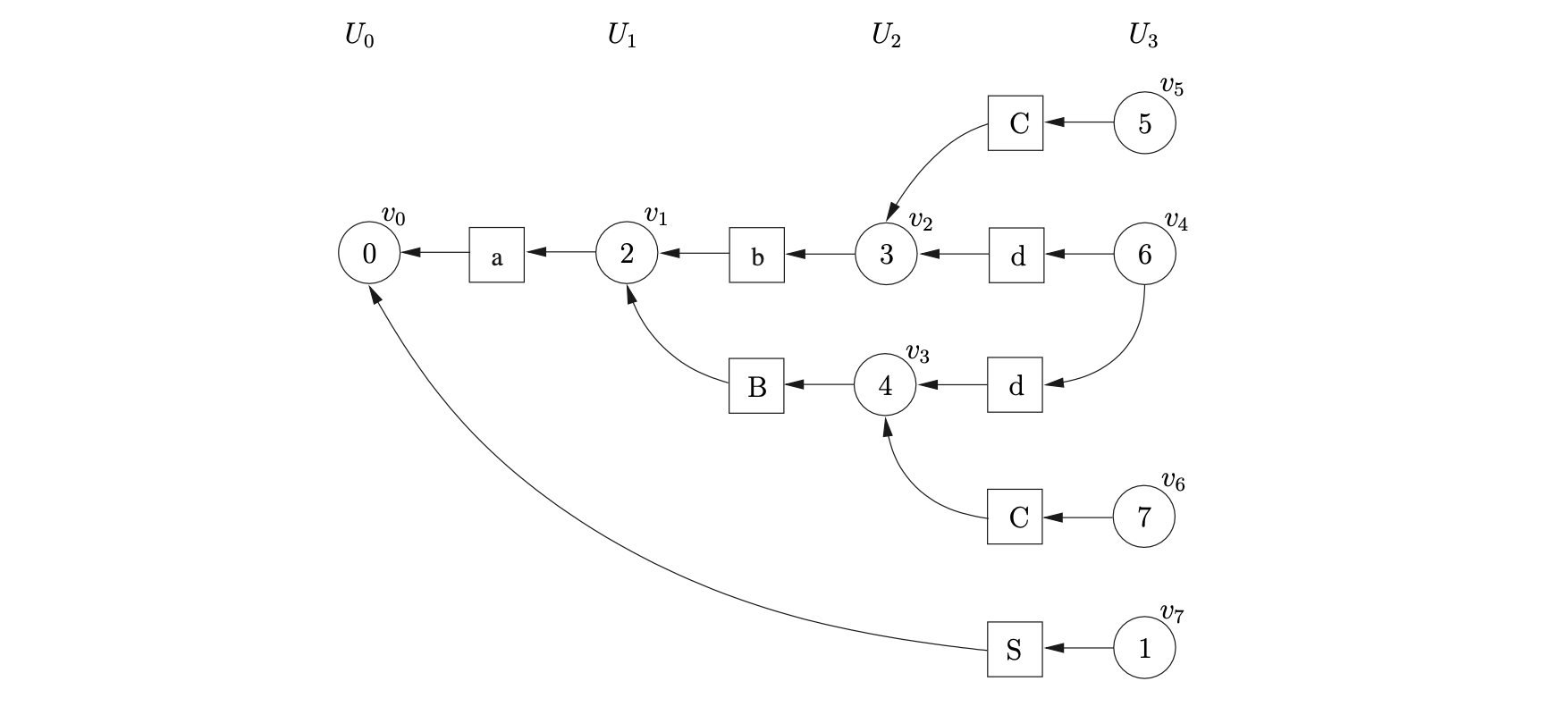
Processing node $v_{7}$ we find the accept action $acc\in\mathcal{T}(1,\$)$. Since we have consumed all of the input and processed all state nodes in the current level the input string $abc$ is accepted.

Note that it is a property of the GSS that all symbol nodes pointed to by a state are labelled by the same grammar symbol.

4.2.3 Tomita’s Algorithm 1¶

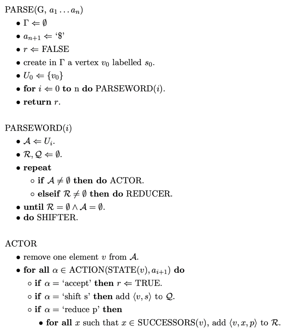
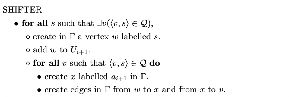
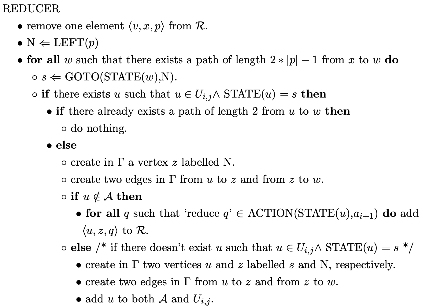
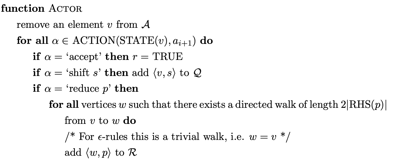
Tomita’s Algorithm 1 basically works by constructing a GSS in the way we have described in the previous section. However, as is shown in the previous example there may be more than one node in the frontier of the GSS waiting to be processed. Tomita uses a special bookkeeping set, $\mathcal{A}$, to keep track of these newly created state nodes. A parse is performed by iterating over this set and finding all applicable actions for a given node. However, as it is possible for a node to have multiple applicable actions (as a result of a conflict in the parse table) two additional bookkeeping sets, $\mathcal{Q}$ and $\mathcal{R}$, are used to store any pending shifts and reductions. The set $\mathcal{Q}$ stores elements of the form $(v,k)$, where $v$ is the node labelled $h$ that has a transition labelled by the next input symbol to a state $k$ in the DFA.

Before describing the elements stored in the set $\mathcal{R}$ we discuss how reductions are performed in the GSS. Recall that the standard LR parser performs a reduction for a rule $A::=X_{1}\ldots X_{j}$ by popping $j$ symbols off the top of the stack. In comparison a reduction in a GLR parser is associated with a node in the frontier and requires all paths of length $2j$ to be traced back from the given node. In the worst case this search may require $O(n^{j})$ time.

The efficiency of Tomita’s algorithms stems from the fact that the same part of the input is not parsed more than once in the same way. In other words, each reduction path is only traversed once for each reduction. However, it is possible for a new edge to be added to an existing node in the frontier that has already performed its associated reductions. This new edge introduces a new reduction path that needs to be traversed for the parse to be correct. So as not to traverse the same path more than once Tomita stores elements of the form $(w,t)$, where $t$ is the rule number of the reduction in the set $\mathcal{R}$ and $w$ is the first edge of the path down which reduction $t$ is to be applied.

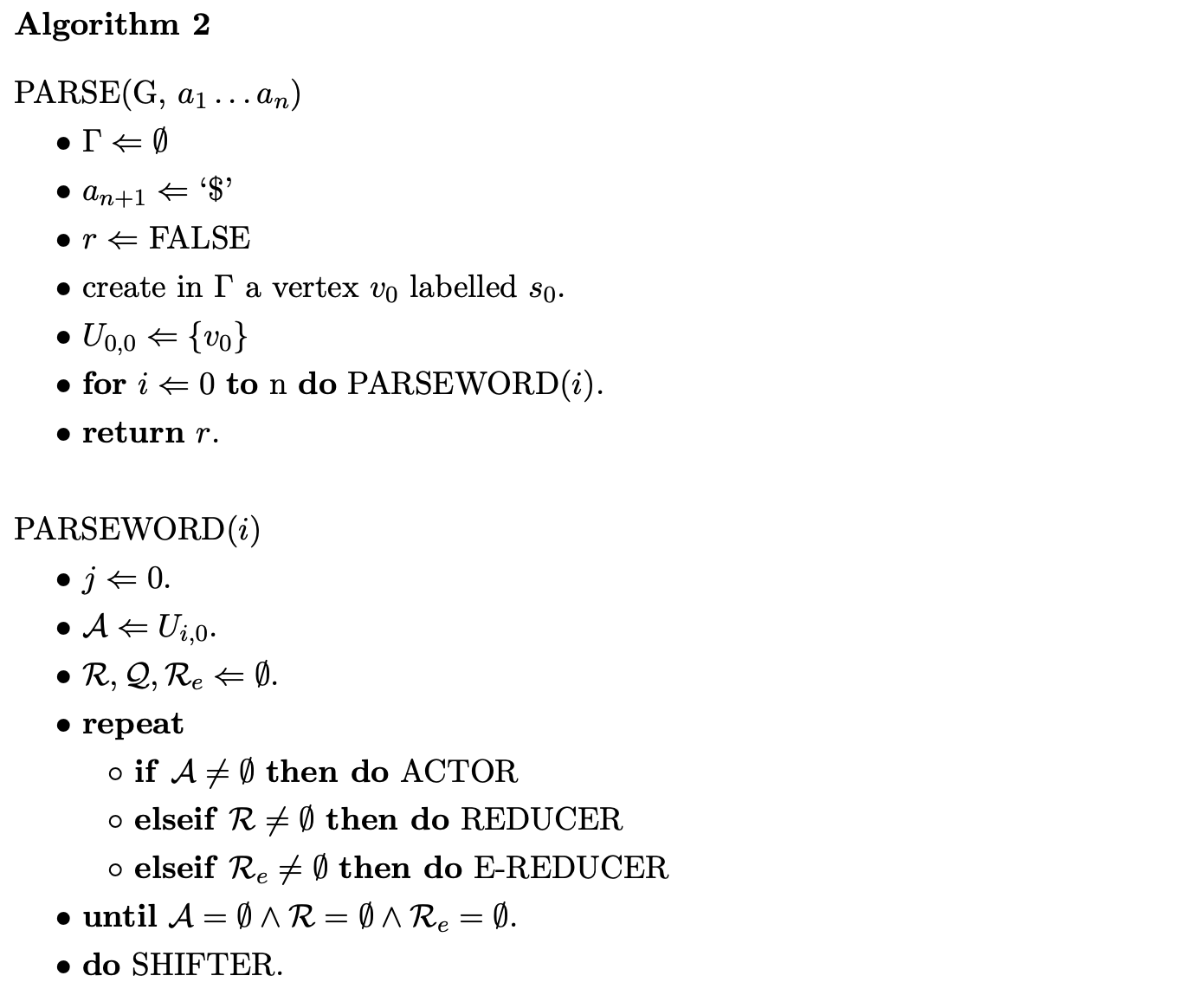
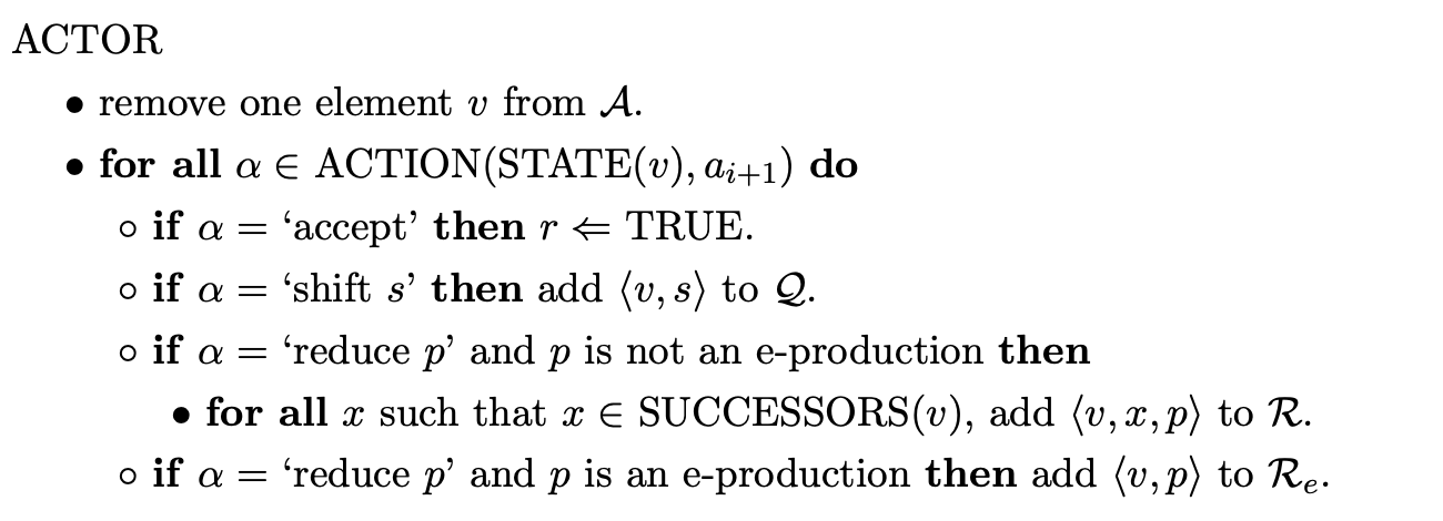
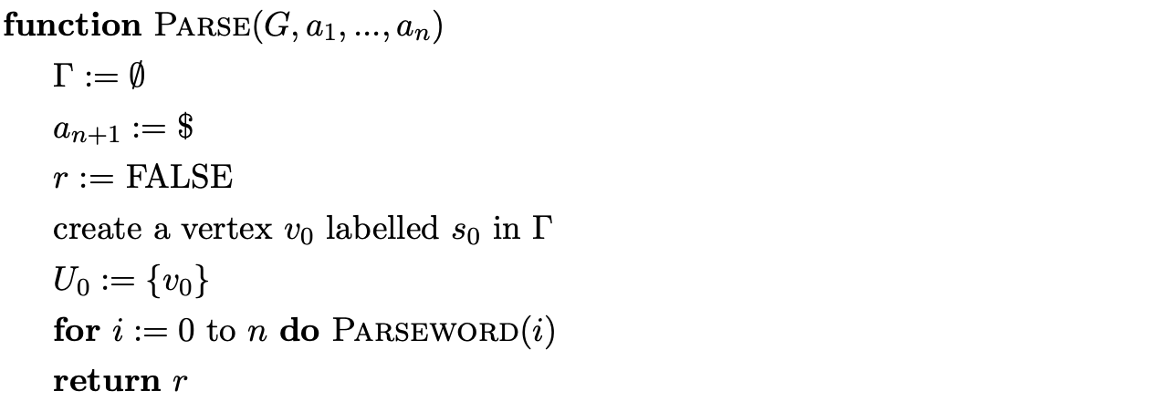
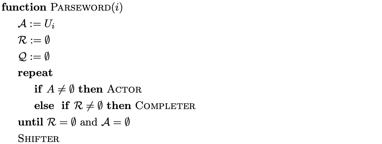
Below is the formal description of Tomita’s Algorithm 1, taken from [Tom86].

4.2.4 Parsing with $\epsilon$-rules¶

Tomita’s Algorithm 1 is defined to work on $\epsilon$-free grammars and hence does not contain the machinery to deal with $\epsilon$-rules. However, by modifying the way reductions are performed, the algorithm can parse grammars containing $\epsilon$-rules. Recall that when a new node, $v$, is created whose state contains an applicable reduction for a rule of the form $A::=\alpha$, the algorithm finds all nodes at the end of the paths of length $2\times|\alpha|-1$ from the successors of $v$. Since $\epsilon$-rules have length zero, an $\epsilon$-reduction does not require a path to be traversed.

Although it is trivial to extend Algorithm 1 to deal with $\epsilon$-rules, the straightforward approach fails to parse certain grammars correctly. For example, consider Grammar 4.2 and the string $aab$. The associated LR(1) DFA is shown in Figure 4.2.

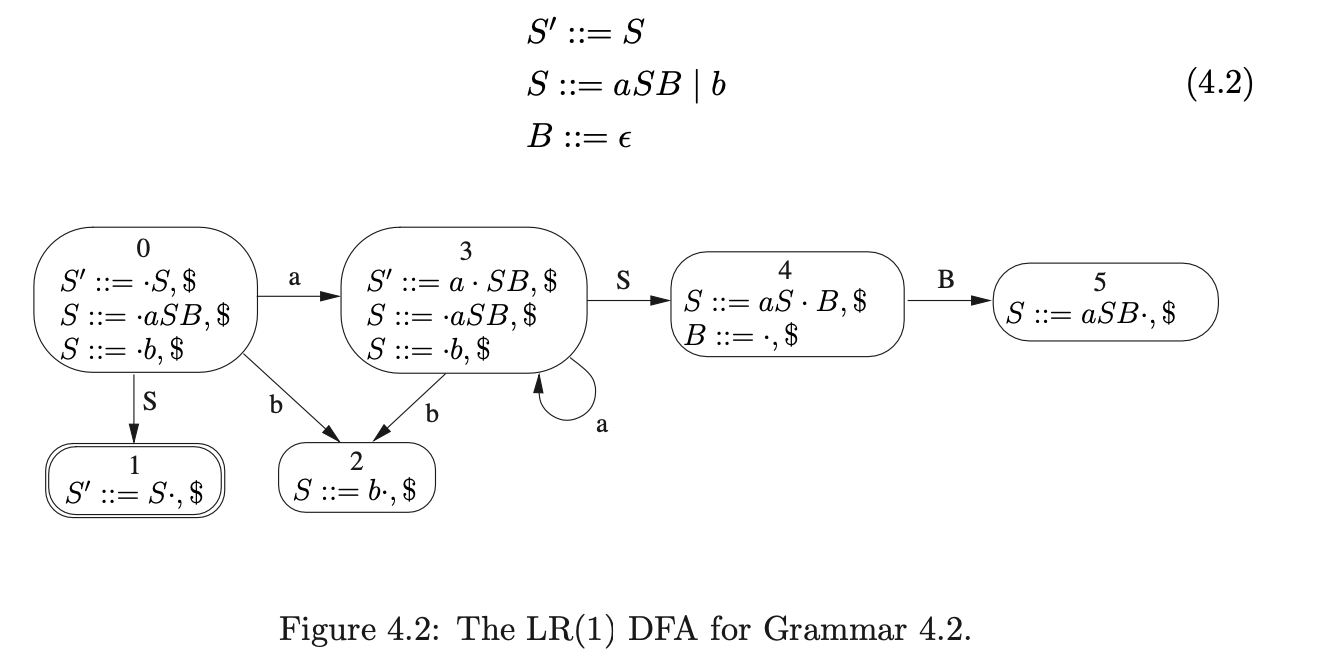
We begin the parse by creating $v_{0}$ and adding it to $U_{0}$ and the set $\mathcal{A}$. When $v_{0}$ is processed in the Actor we only find a shift to state 3 on the first input symbol $a$. We create a new symbol node labelled $a$ which we make a successor of $v_{1}$ and a predecessor of $v_{0}$.

We continue in this way shifting the next two input symbols and constructing the GSS shown below.

Processing $v_{3}$, we find the reduction on rule 2, $S::=b$, which is applicable from state 2. From the only successor of $v_{3}$, the symbol node labelled $b$, we traverse a path of length one to $v_{2}$. We then create the new state node $v_{4}$, labelled $4$, and a new path of length two between $v_{4}$ and $v_{2}$ via a new symbol node labelled $S$.

From state $4$ there is only one applicable reduction on rule $3$, $B::=\epsilon$. Since the right hand side of the rule is $\epsilon$, we do not traverse a reduction path. This results in the creation of $v_{5}$ with a path to $v_{4}$ via a the new symbol node labelled $B$.

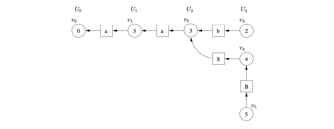Processing $v_{5}$, we find a reduction on rule $1$, $S::=aSB$. We trace back a path of length $5$ to $v_{1}$ from the successor of $v_{5}$. Since the node $v_{4}$, which is labelled by the goto state of the reduction, already exists in the frontier of the GSS a new path of length two is added from $v_{4}$ to $v_{1}$ via a new symbol node labelled $S$.

At this point there are no nodes waiting to be processed and no actions are queued in either of the bookkeeping sets $\mathcal{Q}$ or $\mathcal{R}$. Although all the input has been consumed the parse terminates in failure since there is not a state node in the frontier of the GSS that is labelled by the accept state of the DFA. This is clearly incorrect behaviour since the string $aab$ is in the language of Grammar 4.2.

It turns out that the problem is caused by the new reduction paths created by nullable reductions. Recall that when a new edge is added from an existing node in the GSS, Algorithm 1 re-performs any reductions that have already been applied from $v$. However, in the above example the new path of length two from $v_{4}$ to $v_{1}$ did not create a new reduction path from $v_{4}$, but it did from $v_{5}$.

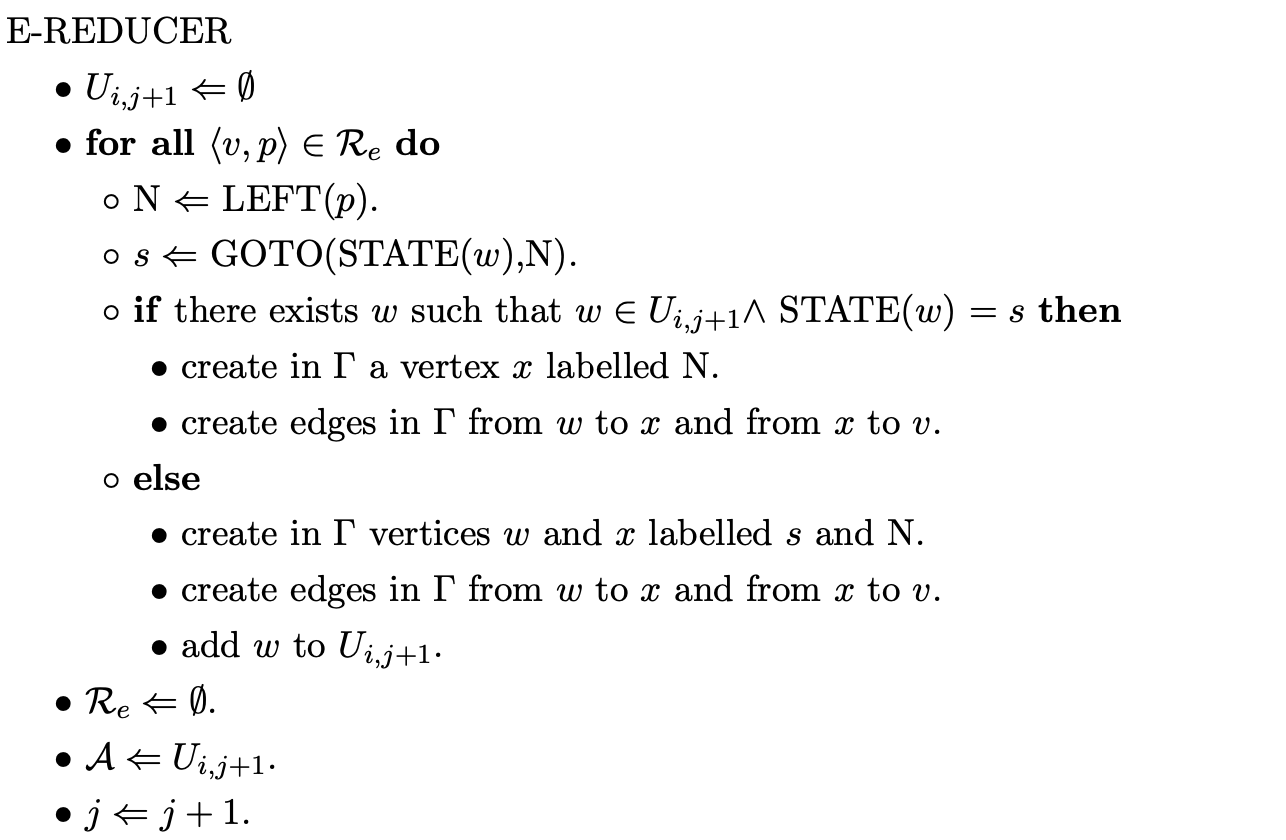
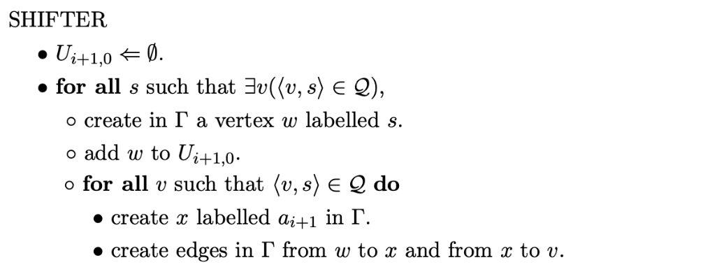
We discuss this problem in more detail in Chapter 5. Tomita deals with this problem in Algorithm 2 by introducing sub-levels to the GSS. When an $\epsilon$-reduction is performed a new sub-frontier is created and the node labelled by the goto state of the reduction is created in this new sub-frontier. Before presenting the formal specification of Algorithm 2, we demonstrate its operation using the above example once again.

4.2.5 Tomita’s Algorithm 2¶

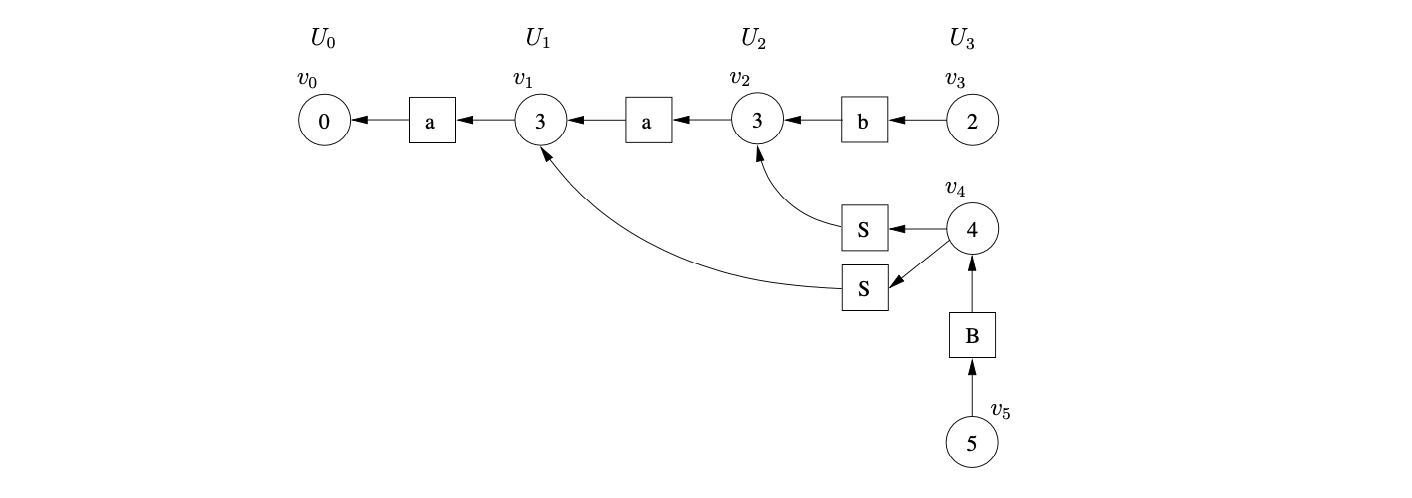
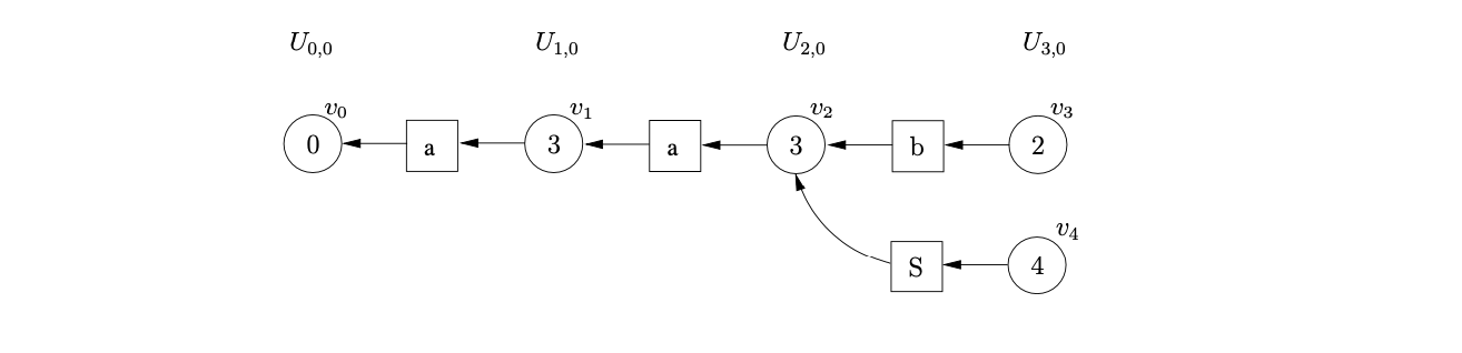
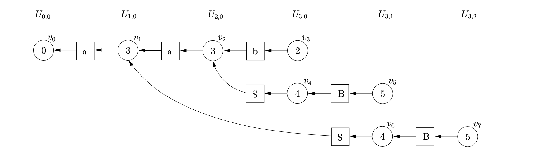
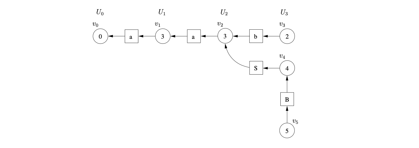
Tomita’s Algorithm 2 creates sub-frontiers $U_{i,j}$ in $U_{i}$ when $\epsilon$-reductions are applied. To parse the string $aab$ we begin by creating $v_{0}$, labelled with the start state of the DFA, in level $U_{0,0}$. The only applicable action from state 0 of the DFA is a shift to state 3 on the first input symbol, $a$. We read the $a$ from the input string, create the symbol node labelled $a$ and the state node $v_{1}$, labelled 3. We make the new symbol node a successor of $v_{1}$ and a predecessor of $v_{0}$. The GSS constructed up to this point is shown below.

We continue in this way, reading the next two input symbols and constructing the GSS shown below.

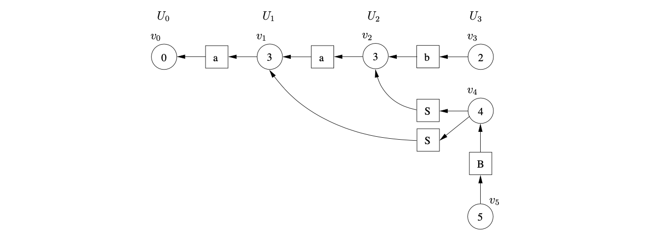
At this point state 2 contains a reduction on rule $S::=b$. We perform the reduction by traversing a path of length two from $v_{3}$ to $v_{2}$. Since there is no node labelled by the goto state of the reduction we create $v_{4}$, the symbol node labelled $S$ and the new path from $v_{4}$ to $v_{2}$.

The only applicable action in state 4 is the nullable reduction on rule $B::=\epsilon$. Since it is nullable reductions that cause new edges to be added to existing nodes, a new sub-frontier $U_{3,1}$ is created. We create the symbol node labelled $B$ and the state node, $v_{5}$, in $U_{3,1}$. We make the new symbol node a successor of $v_{5}$ and a predecessor of $v_{4}$.

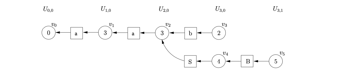
We then continue as normal processing any applicable actions from state 5. We trace back a path of length six for the reduction on rule $S::=aSB$. Because the reduction is performed from a state node in the sub-frontier $U_{3,1}$ we also create the state node $v_{6}$, labelled by the goto state of the reduction in $U_{3,1}$.

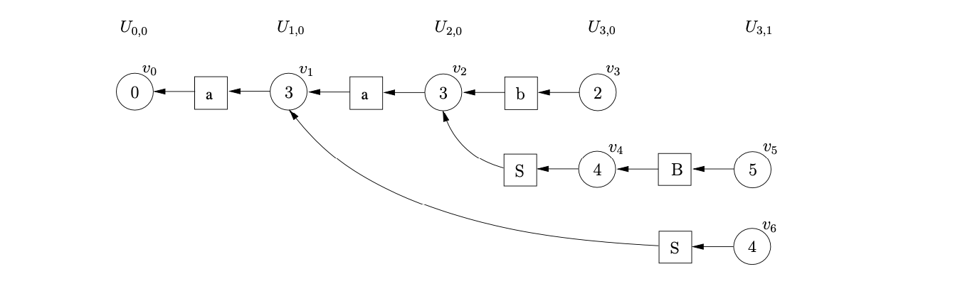
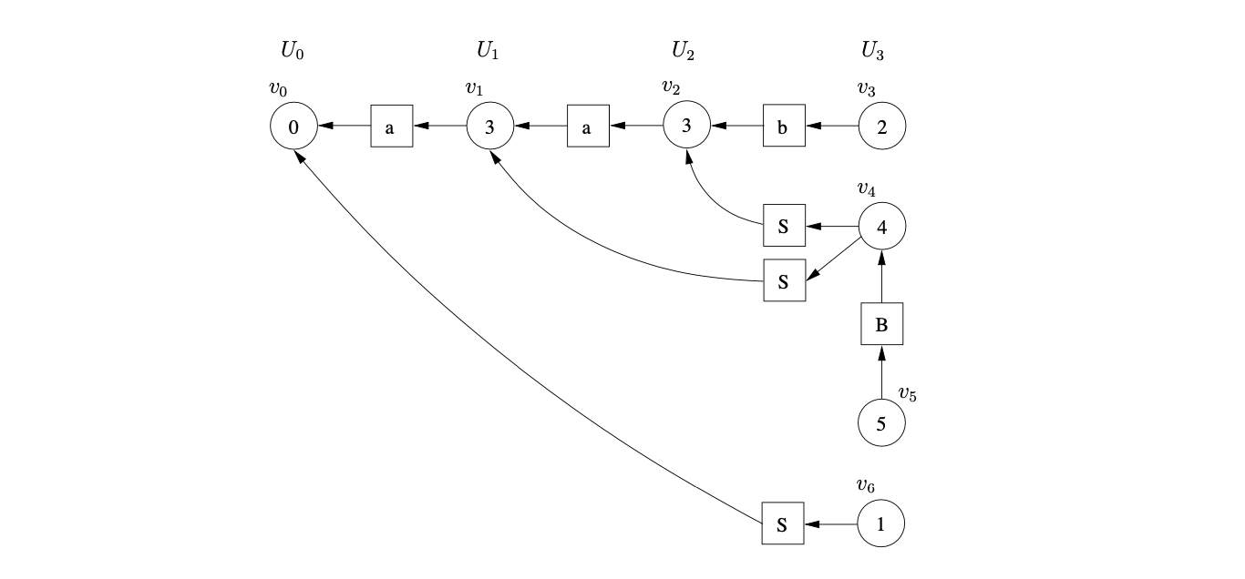
From state 4 we can perform another nullable reduction on rule $B::=\epsilon$. As a result we create a new sub-frontier, $U_{3,2}$, and add, $v_{7}$, the state node labelled by the goto state of the reduction to it.

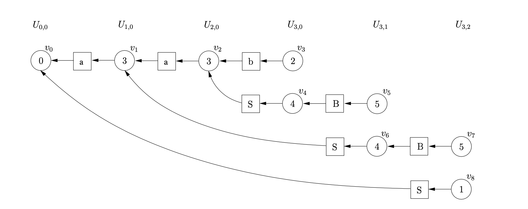
Performing the reduction from $v_{7}$ on rule $S::=aSB$, we trace back a path to $v_{0}$. We create, $v_{8}$, labelled 1, and the symbol node labelled $S$. We make the symbol node a successor of $v_{8}$ and a predecessor of $v_{0}$. Since $v_{8}$ is labelled by the accept state of the DFA and we have consumed all the input string, the parse is successful. The final GSS constructed is shown below.

The non-termination of Algorithm 2¶

Although Algorithm 2 is defined to work on grammars containing $\epsilon$-rules, it can fail to terminate when parsing strings with hidden-left recursive grammars. For example, consider the parse for the string $ab$ with Grammar 4.3 and the LR(1) DFA in Figure 4.3.

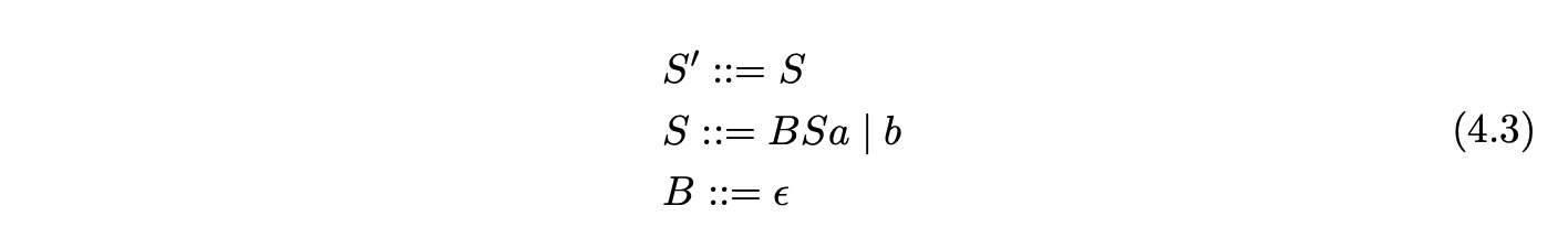
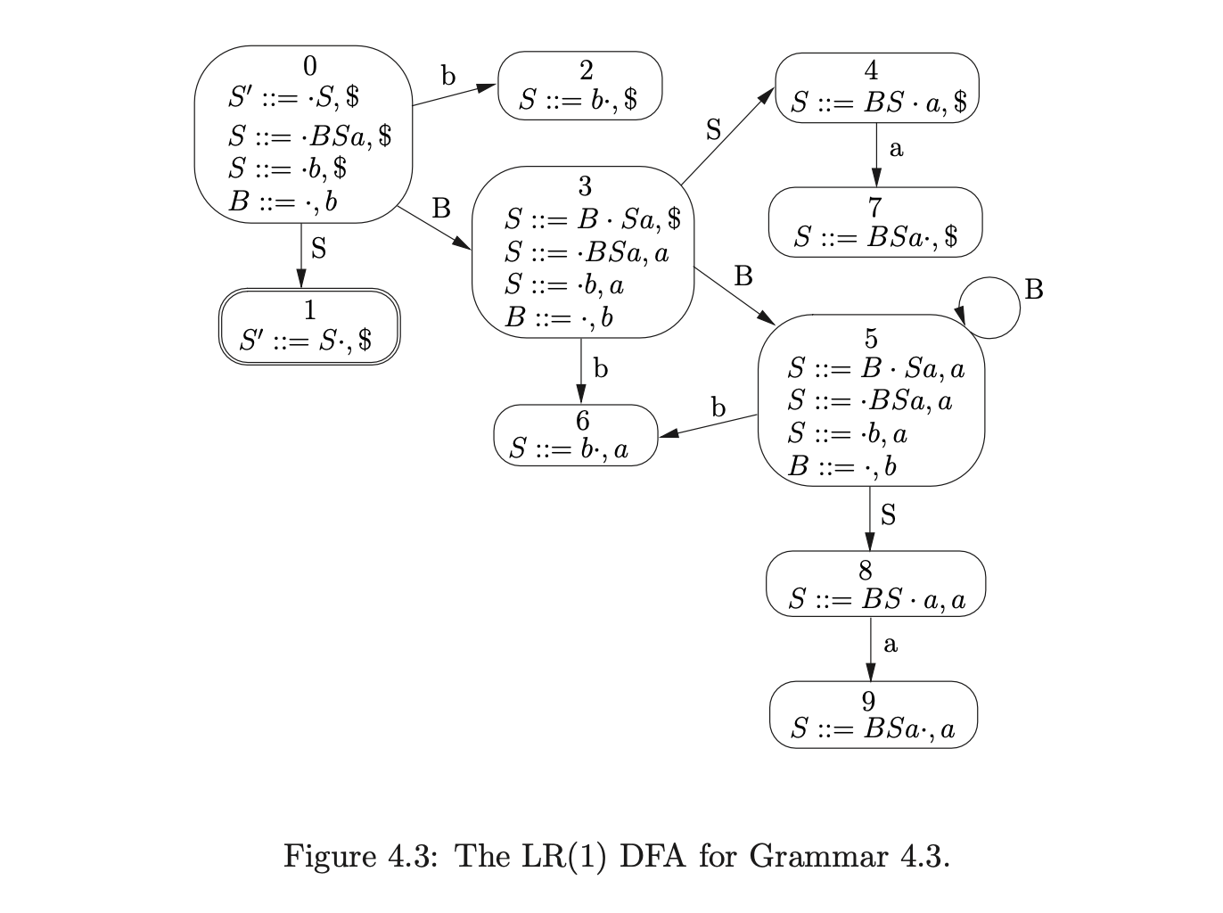We begin the parse, as usual, by creating $v_{0}$ in level $U_{0,0}$. Since state $0$ contains a shift/reduce conflict, we queue the shift and perform the reduction on rule $B::=\epsilon$. Since the reduction is nullable we construct a new sub-frontier $U_{0,1}$ with the new state node, $v_{1}$, labelled $3$ and a path of length two from $v_{1}$ to $v_{0}$, via the new intermediate symbol node labelled $B$.

State 3 contains another shift/reduce conflict, so we queue the shift and perform the reduction $B::=\epsilon$ once again. Since this reduction is also nullable we create $U_{0,2}$, $v_{2}$ and a path of length two from $v_{2}$ to $v_{1}$ via the intermediate symbol node $B$.

Processing $v_{2}$, we find the same shift/reduce conflict in state 5; a shift on $b$ and the nullable reduction on rule $B::=\epsilon$. Performing this reduction results in yet another new sub-frontier and another state node labelled 5. This process continues indefinitely preventing the algorithm from terminating.

In the next section we discuss a modification of Algorithm 2 that enables the parser to work for all context-free grammars.

4.3 Farshi’s extension of Algorithm 1¶

The non-termination of Tomita’s Algorithm 2 was first reported by Nozohoor-Farshi. In [10], Farshi attributes the problem of Algorithm 2 to the false assumption that only a finite number of nullable reductions can be applied between the shift of two consecutive input symbols. Instead of creating sub-frontiers for nullable reductions, Farshi introduces extra searching when a new edge is added from an existing node in the frontier of the GSS.

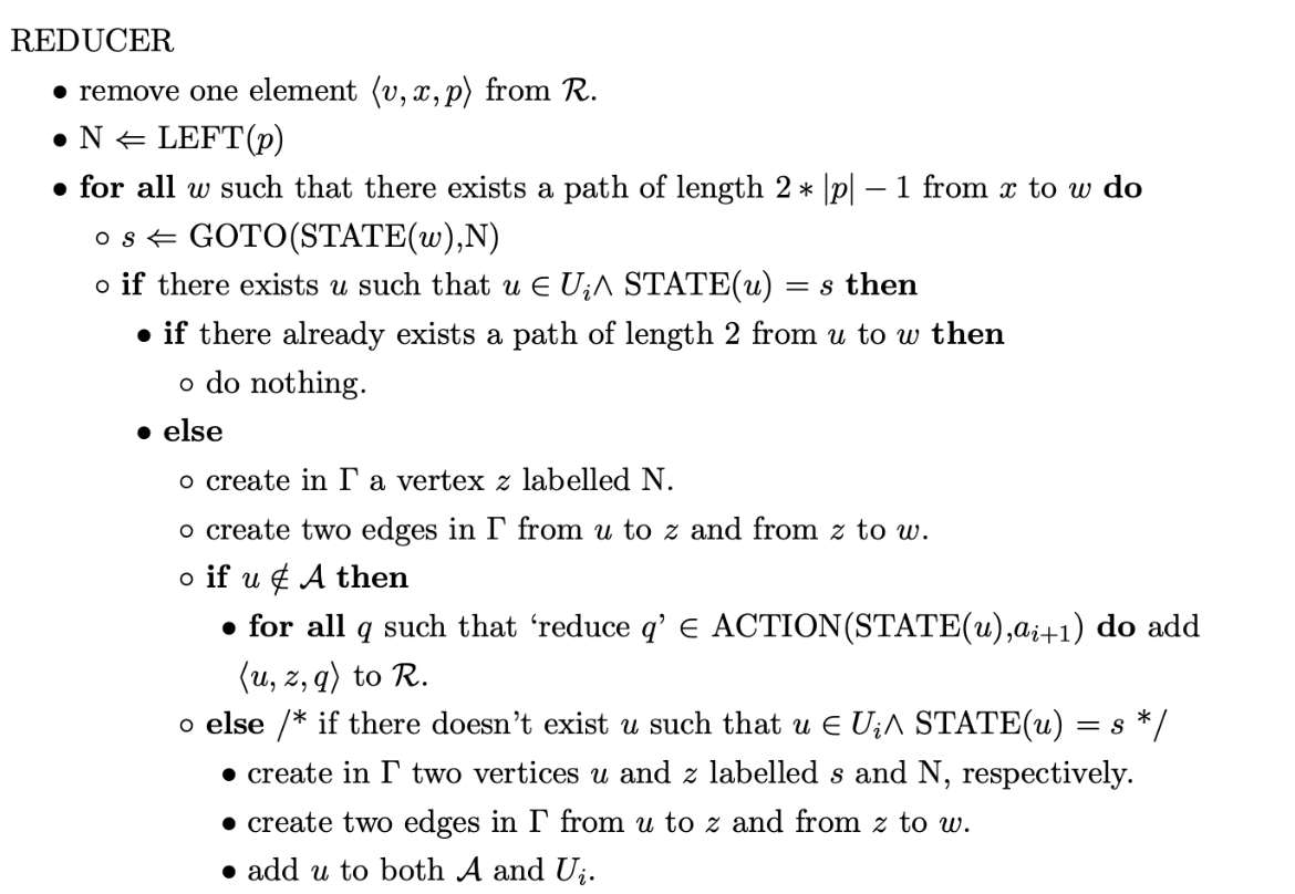
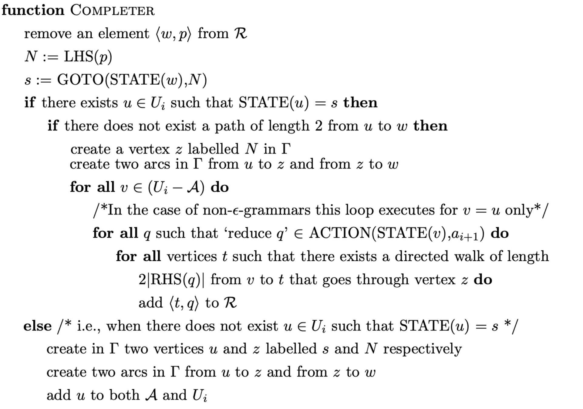
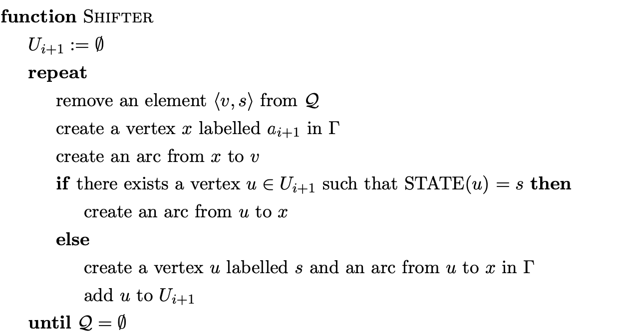
In this section we describe the operation of Farshi’s correction and highlight the extra costs involved. The formal specification of the algorithm is taken from [10]. The layout and notation of the algorithm is similar to that of Tomita’s, apart from the Reducer function which is renamed to Completer.

Farshi’s recogniser¶

Variables $$ \begin{array}{l} \Gamma: \ \text{The parse graph.} \\ U_{i}: \text{The set of state vertices created just before shifting the input word } a_{i+1} .\\ s_{0}: \ \text{The initial state of the parser.} \\ \mathcal{A}: \ \text{The set of active nodes on which the parser will act.} \\ \mathcal{Q}: \ \text{The set of shift operations to be carried out.} \\ \mathcal{R}: \ \text{The set of reductions to be performed.} \\ \end{array} $$

4.3.1 Example - a hidden-left recursive grammar¶

Consider the parse of the string $ba$ (with Grammar 4.3) that caused $\text{Tomita's Algorithm} 2$ to fail to terminate in the previous section. We demonstrate how Farshi’s algorithm deals with hidden-left recursive grammars by tracing the construction of the $GSS$.

We create $v_{0}$, labelled by the start state of the $DFA$, in level $U_{0}$. Since there is a shift/reduce conflict in state 0, we queue the shift and perform the reduction on rule $B::=\epsilon$. The reduction is nullable so we create the new state node, $v_{1}$ labelled 3, in the current level, and a path of length two from $v_{1}$ to $v_{0}$ via the new intermediate symbol node $B$.

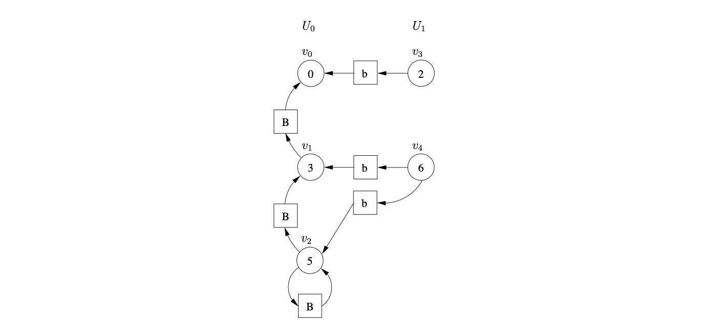
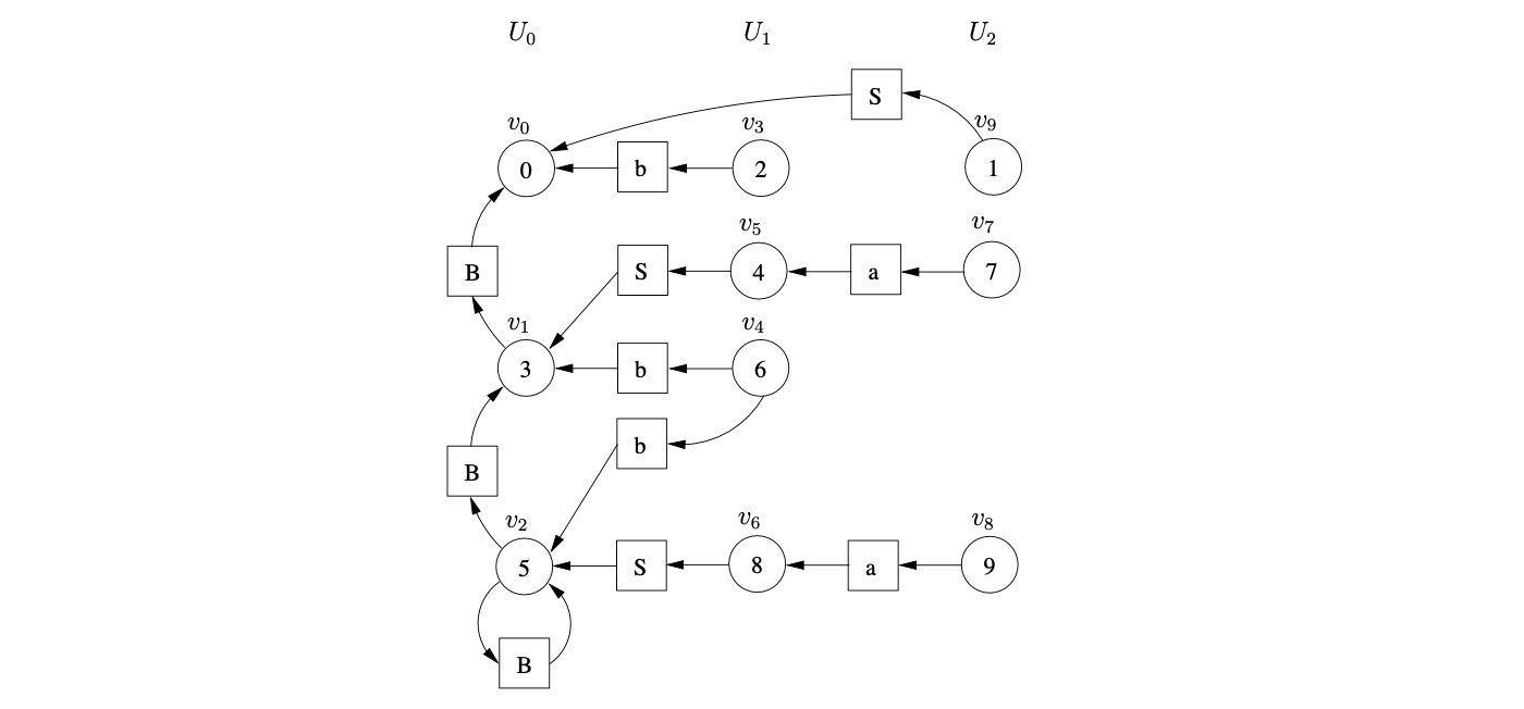
There is another shift/reduce conflict in state 3, so we queue the shift once again and perform the reduction on rule $B::=\epsilon$. As a result we create $v_{2}$ in the current level and another symbol node labelled $B$. We make this new symbol node a successor of $v_{2}$ and a predecessor of $v_{1}$. There is the same shift/reduce conflict in state 5, so we perform the nullable reduction and queue the shift action again. However, because of the loop in state 5 of the DFA, caused by the hidden-left recursive rule $S::=BSa$, we create a cyclic path of length two from $v_{2}$ to itself via a new symbol node labelled $B$.

There are no further reductions that can be performed from any of the state nodes in level $U_{0}$, so we proceed to carry-out the queued shift actions. This results in two new state nodes, $v_{3}$ and $v_{4}$, being created in level $U_{1}$, with paths of length two, via three separate symbol nodes labelled $b$, back to the appropriate nodes in level $U_{0}$.

From this point on Farshi’s algorithm behaves in the same way as Tomita’s Algorithm 2. Once all actions have been performed the GSS shown below is constructed.

Since $v_{9}$ is labelled by the accept state of the DFA and we have consumed all the input string, we have successfully recognised $ba$ as being in the language of Grammar 4.3.

4.3.2 Example - a hidden-right recursive grammar¶

It is claimed that Farshi’s algorithm “…works exactly like the original one [Tomita’s] in case of grammars that have no $\epsilon$-productions… [and] has no extra costs beyond that of the original algorithm.” [NF91, p.74].

Although it is possible to implement the algorithm so as not to incur the extra searching costs for $\epsilon$-free grammars the algorithmic description presented in [NF91] does not include any functionality to achieve it. The only indication that this is possible comes from the comment in the Completer function.

The extra searching costs introduced by Farshi’s modification can be high if done naively. The algorithm, as described in [15], searches all nodes in the current frontier that are not waiting to be processed, and finds any reduction paths that pass through the new node created as part of the original reduction. This extra searching to correct Tomita’s error for grammars containing right nullable rules effectively defeats the core of Tomita’s idea - reduced graph searching. This fix can be thought of as a brute force way to fixing the problem.

To highlight the extra searching introduced by Farshi’s algorithm we demonstrate its operation for the parse of the string $aab$ with Grammar 4.2 shown on page 4.2. We begin by creating the start state, $v_{0}$, in $U_{0}$. We add $v_{0}$ to the set $\mathcal{A}$ and process it in the Actor. As there is only a shift to state $3$, from state $0$ on an $a$, $(v_{0},3)$ is added to $\mathcal{Q}$. We then create the state node $v_{1}$ in $U_{1}$, the symbol node labelled $a$ and a path of length two from $v_{1}$ to $v_{0}$ via the symbol node.

We parse the next two input symbols in this way, creating the two new state nodes $v_{2}$ and $v_{3}$.

When we process $v_{3}$ in the Actor we find the reduction on rule $2$, ($S::=b\cdot$), in state $2$. We trace back a path of length two from $v_{3}$ to $v_{2}$ and add $(v_{2},2)$ to $\mathcal{R}$. We process the contents of $\mathcal{R}$ in the Completer which results in the new node, $v_{4}$, labelled $4$, being created in $U_{3}$, with a path of length two to $v_{2}$ through a new symbol node labelled $S$.

Processing $v_{4}$ in the Actor we find an applicable reduction on rule $3$, ($B::=\cdot$). Since the reduction is nullable, we do not traverse any edges and add $(v_{4},3)$ to the set $\mathcal{R}$. When we process $(v_{4},3)$ in the Completer we create the new node, $v_{5}$, labelled $5$, and add it to the set $\mathcal{A}$ and $U_{3}$. We create the symbol node labelled $B$ and a path of length two from $v_{5}$ to $v_{4}$ via the new symbol node.

When we process $v_{5}$ we find the reduction on rule 1, $(S::=aSB\cdot)$, in state 5. We trace back a path of length six to $v_{1}$ and add $(v_{1},1)$ to $\mathcal{R}$. When we process $(v_{1},1)$ in the Completer, we find that there is already a node labelled 4 in the frontier of the GSS. As there is not a path of length two to $v_{1}$ from $v_{4}$, we create one via a new symbol node labelled $S$. However, because we have added a new edge to an existing node of the GSS we need to ensure that no new reduction paths have been introduced from the other nodes in the frontier. This is achieved by effectively traversing all reduction paths from the existing nodes in the frontier and re-performing any reductions that go through the new edge.

It is not necessary to re-trace reduction paths from nodes that are still waiting to be processed, as they will be carried out later. However, since there are no nodes in the set $\mathcal{A}$ at this point of our example, the set difference $U_{3}-\mathcal{A}$, results in all nodes in $U_{3}$ being considered. We trace the paths:

$v_{3},v_{2}$ for reduction $(S::=b\cdot)$;
$v_{5},v_{4},v_{2},v_{1}$ for reduction $(S::=aSB\cdot)$;
$v_{5},v_{4},v_{1},v_{0}$ for reduction $(S::=aSB\cdot)$.

Only the last traversal goes through the new edge between $v_{4}$ and $v_{1}$, so we add $(v_{0},1)$ to $\mathcal{R}$ for the reduction on rule 1.

When we perform the reduction in the Completer we create the new node, $v_{6}$, labelled 1, and the symbol node labelled $S$ with a path from $v_{6}$ to $v_{0}$. Since $v_{6}$ is labelled by the accept state of the DFA and we have consumed all the input string, the parse terminates in success. The final GSS constructed is shown below.

In practice this searching can trigger considerable extra work, see Chapter 10 where we discuss some experiments. It turns out that it is trivial to improve the efficiency of the algorithm by limiting the searching to paths within the current level. This is possible as the new path created from the reduction has to leave the current frontier. As soon as a path being searched goes to a previous level and does not go through the new edge, that particular search can be terminated.

We have implemented both the naive and optimised versions of Farshi’s algorithm. We compare both versions to each other in Chapter 10.

In the next section we discuss the construction of derivations by GLR parsers, specifically focusing on Tomita’s approach and Rekers’ modifications.

4.4 Constructing derivations¶

The GLR algorithm finds all possible parses of an input string. This is because Tomita was interested in natural language processing which often has “temporarily or absolutely ambiguous input sentences” and hence requires this approach to deal with it. Tomita recognised the problem of ambiguous parsing leading to exponential time requirements. The number of parses of a sentence with an ambiguous grammar may grow exponentially with the size of the sentence [10]. Therefore an efficient parsing algorithm would still require exponential time just to print the exponential number of possible parse trees. The key is to use an efficient representation of the parse trees. Tomita achieved this through subtree sharing and local ambiguity packing of the parse forest.

In this section we define the structure used by Tomita to represent all derivations of an input string and then discuss his parsing algorithm and Rekers’ subsequent extension.

4.4.1 Shared packed parse forests¶

Local ambiguity occurs when there is a reduce/reduce conflict in the parse table. This makes it possible to reduce the same substring in more than one way which manifests itself in the parse tree as two or more nodes with the same label that have leaf nodes representing the same part of the input. A lot of local ambiguity can cause an exponential number of parse trees to be created. However, this can be controlled by combining all parse trees into one structure, taking advantage of sharing and packing of certain nodes, called a Shared Packed Parse Forest (SPPF). The parent nodes are merged into a new node and a packing node is made the parent of each of the subtrees.

For example, consider the ambiguous Grammar 4.4 (previously encountered on page 29), which defines the syntax of simple arithmetic expressions.

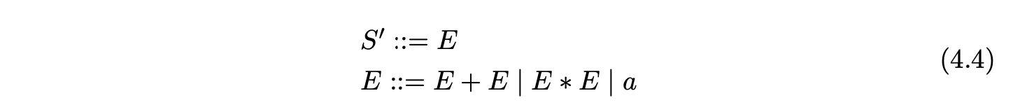
We can parse the string $a+a*a$ in two different ways that represents the left and right associativity of the $*$ symbol. The two parse trees are shown in Figure 4.4.

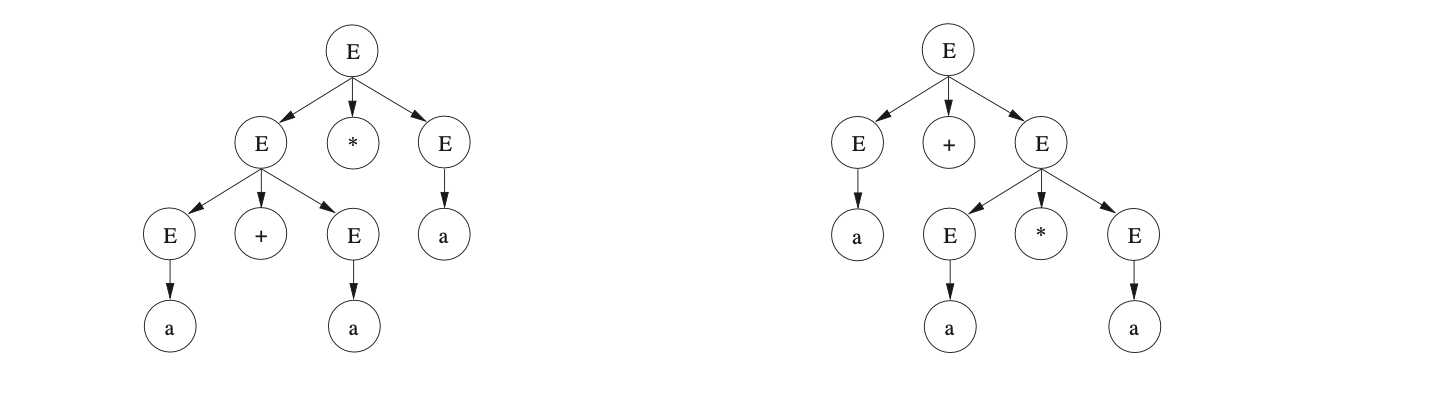
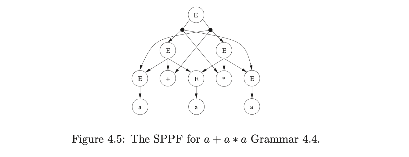
The amount of space required to represent both trees can be significantly reduced by using the SPPF shown in Figure 4.5.

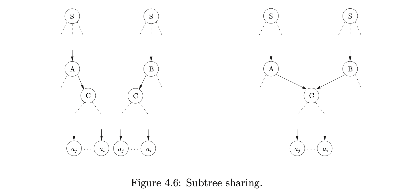
If two trees have the same subtree for a substring $a_{j}\dots a_{i}$ then that subtree can be shared, as is shown in Figure 4.6.

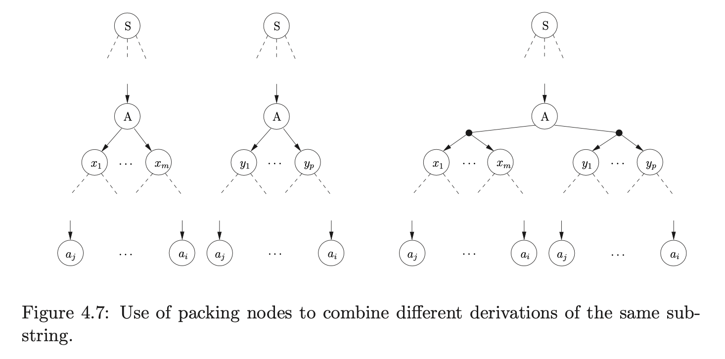
If two trees have a node labelled by the same non-terminal that derives the same substring, $a_{j}\ldots a_{i}$, in two different ways then that node can be packed and the two subtrees added as alternates under the newly packed node. For example, see Figure 4.7 below.

Although the SPPF provides an efficient representation of multiple parse trees it is not the most compact representation possible. It has been shown that maximal sharing can be achieved by “sharing the corresponding prefixes of right hand sides” [1]. This approach involves sharing all nodes that are labelled by the same symbol and derive terminals that are lexicographically the same. However, with this representation the yield of the derivation tree may not be the input string. This technique has been successfully adopted by the SGLR parser in the $\text{Asf+Sdf}$ Meta-Environment [$vdBvDH^{+}01$]. A description of the ATerm library, the data structure that efficiently implements the maximally shared SPPF, is given in [10].

Cyclic grammars

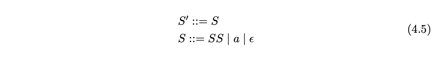
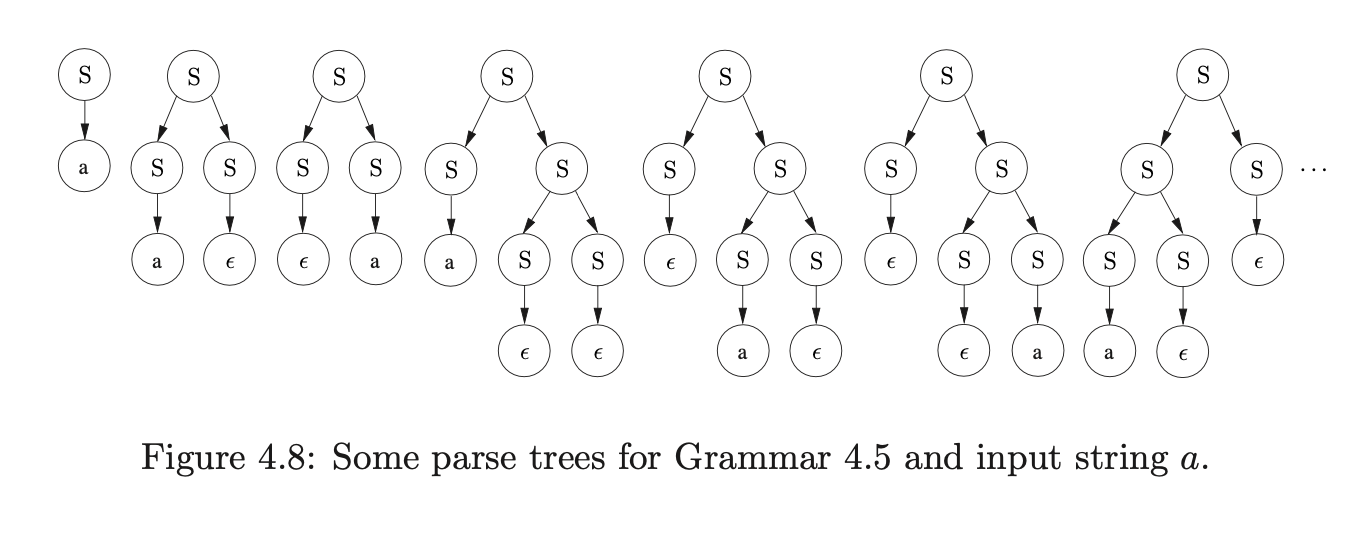
A cyclic grammar contains a nonterminal that can derive itself, $A\stackrel{{*}}{{\Rightarrow}}A$. Cyclic grammars can have an infinite number of derivations for certain strings in their language. For example, the parse of the string $a$ with Grammar 4.5 results in the construction of an infinite number of parse trees of the form shown in Figure 4.8.

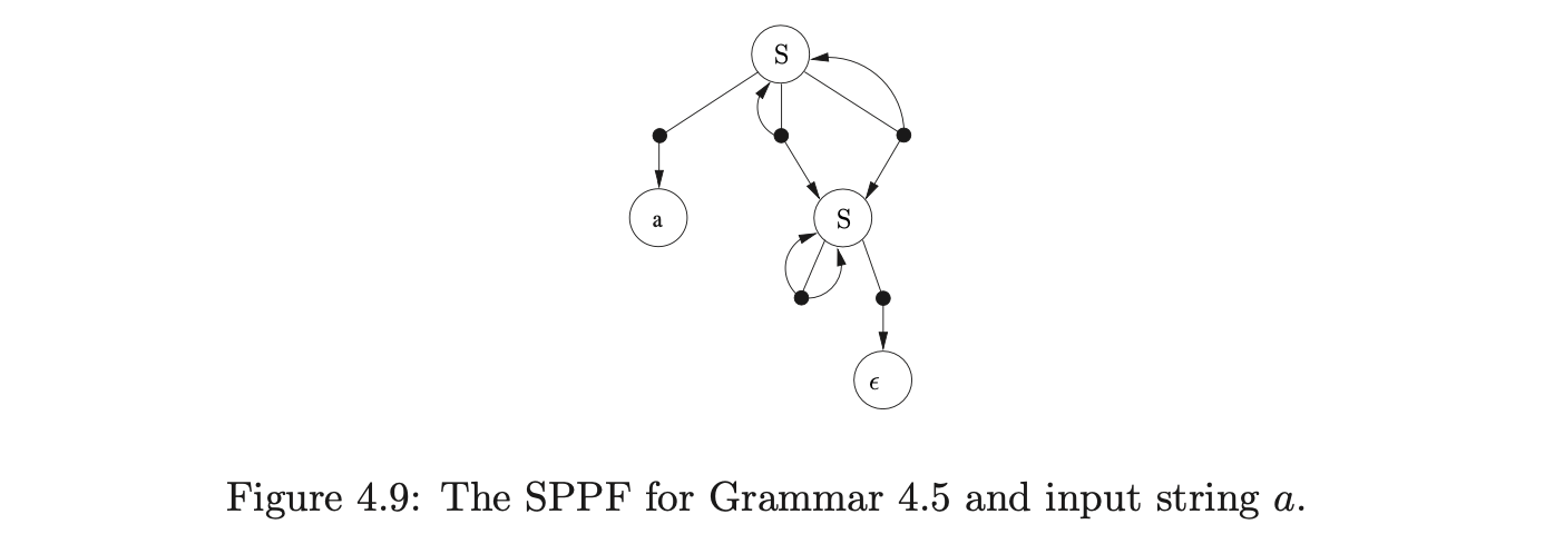
Farshi introduced cycles into the GSS so that his algorithm could be used to parse strings with cyclic grammars. We introduce cycles into the SPPF so that they can be used to represent an infinite number of parse trees. The SPPF representing the parse trees of the above parse is shown in Figure 4.9.

4.4.2 Tomita’s Algorithm 4¶

Tomita’s Algorithm 3 is a recogniser, based on Algorithm 2, that incorporates sharing of symbol nodes into the GSS. Tomita extends Algorithm 3 to a parser, Algorithm 4, by introducing the necessary SPPF construction. Recall that Algorithm 2 can fail to terminate on hidden-left recursive grammars. This behaviour is inherited by Algorithm 4. We discuss the operation of Algorithm 4 to illustrate Tomita’s approach to SPPF generation.

The GSS’s constructed by Tomita’s algorithms contain exactly one symbol node between every connected pair of state nodes. Although the symbol nodes do not perform any specific function in the recognition algorithms, they play an important role in Algorithm 4 - they correspond directly to the nodes in the SPPF.

The amount of space required to represent all derivations of an ambiguous sentence is controlled by the sharing and packing of the nodes in the SPPF. Since the GSS symbol nodes have a one-to-one correspondence with the nodes in the SPPF, some of the symbol nodes in the GSS need to be shared. We demonstrate the construction of an SPPF for the string $abd$ whose Grammar 4.1 and associated LR(1) DFA are shown on page 4.1.

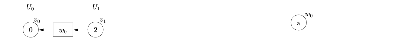
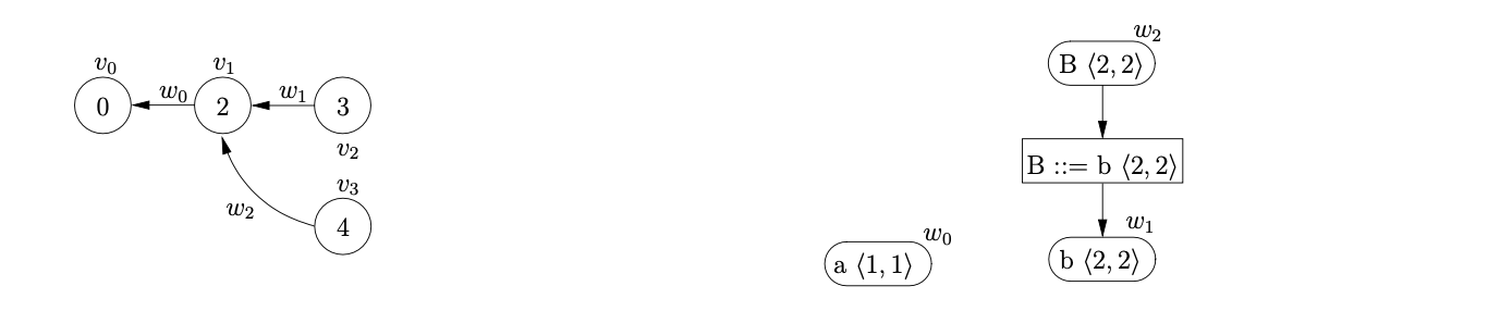
We begin the parse by creating the node $v_{0}$, labelled by the start state of the DFA. The only applicable action from state $0$ is a shift to state $2$ for the first symbol on the input string, $a$. We perform the shift by creating the new state node, $v_{1}$, and the new SPPF node, $w_{0}$, labelled $a$. We use $w_{0}$ as the symbol node on the path from $v_{1}$ to $v_{0}$. To make the example easier to read we draw the SPPF separately from the GSS and only label the GSS symbol nodes with the node of the SPPF.

We continue the parse by processing $v_{1}$ and performing the associated shift to state $3$. We create the new state node, $v_{2}$, labelled $3$, and the new SPPF node, $w_{1}$, labelled $b$, which we use as the symbol node between $v_{1}$ and $v_{2}$.

From state $3$ there is a shift and a reduce action applicable. We queue the shift to state $6$ and perform the reduction on rule $3$, $B::=b$. We begin by tracing back a path of length one from the symbol node $w_{1}$ to $v_{1}$. We then create a new state node, $v_{3}$, labelled $4$ and the new SPPF node, $w_{2}$, labelled $B$. We make $w_{1}$ the child of $w_{2}$ and use $w_{2}$ as the symbol node on the path between $v_{3}$ and $v_{1}$. We process $v_{3}$ and queue the applicable shift action to state $6$ which completes the construction of $U_{2}$.

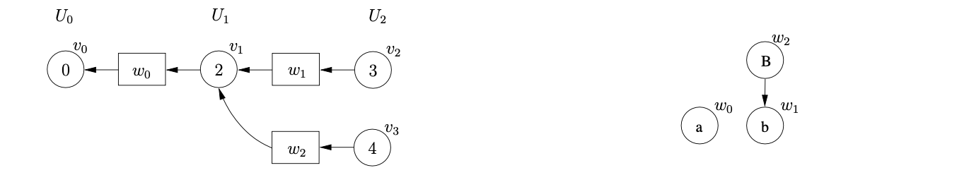
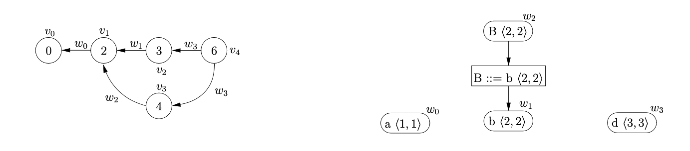
When we perform the two queued shift actions to state $6$, we create a new state node, $v_{4}$, and a new SPPF node $w_{3}$, labelled $d$. We use $w_{3}$ as the symbol node on the path between both $v_{4}$ and $v_{2}$, and $v_{4}$ and $v_{3}$.

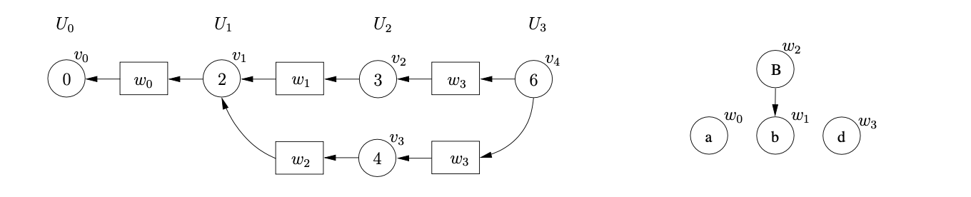
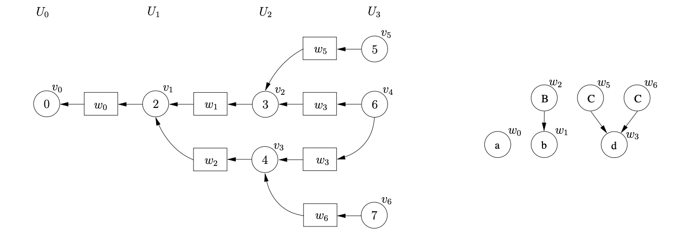
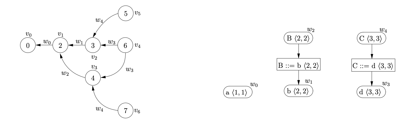
From state 6 there is a reduction on rule 4, $C::=d$, applicable. We trace back the two separate paths of length one from the symbol nodes labelled $w_{3}$ which lead to $v_{2}$ and $v_{3}$ respectively. For the reduction path that leads to $v_{2}$ we create the new state node $v_{5}$, labelled 5, and the new SPPF node, $w_{5}$, labelled $C$. We make the symbol node, $w_{3}$, the child of $w_{5}$ and use $w_{5}$ as the symbol node between $v_{5}$ and $v_{2}$. For the second reduction path we create the state node $v_{6}$ and another SPPF node $w_{6}$, also labelled $C$ with $w_{3}$ as its child.

Processing $v_{5}$ we find that the reduction on rule 1, $S::=abC$, is applicable. We trace back a path of length five from $w_{5}$ to $v_{0}$ and collect the SPPF nodes $w_{1}$ and $w_{0}$ encountered on the traversal. We create the new state node $v_{7}$, labelled 1, and the new SPPF node, $w_{7}$, labelled $S$. We make $w_{0},w_{1}$ and $w_{5}$ the children of $w_{7}$ and use $w_{7}$ as the symbol node on the path between $v_{7}$ and $v_{0}$.

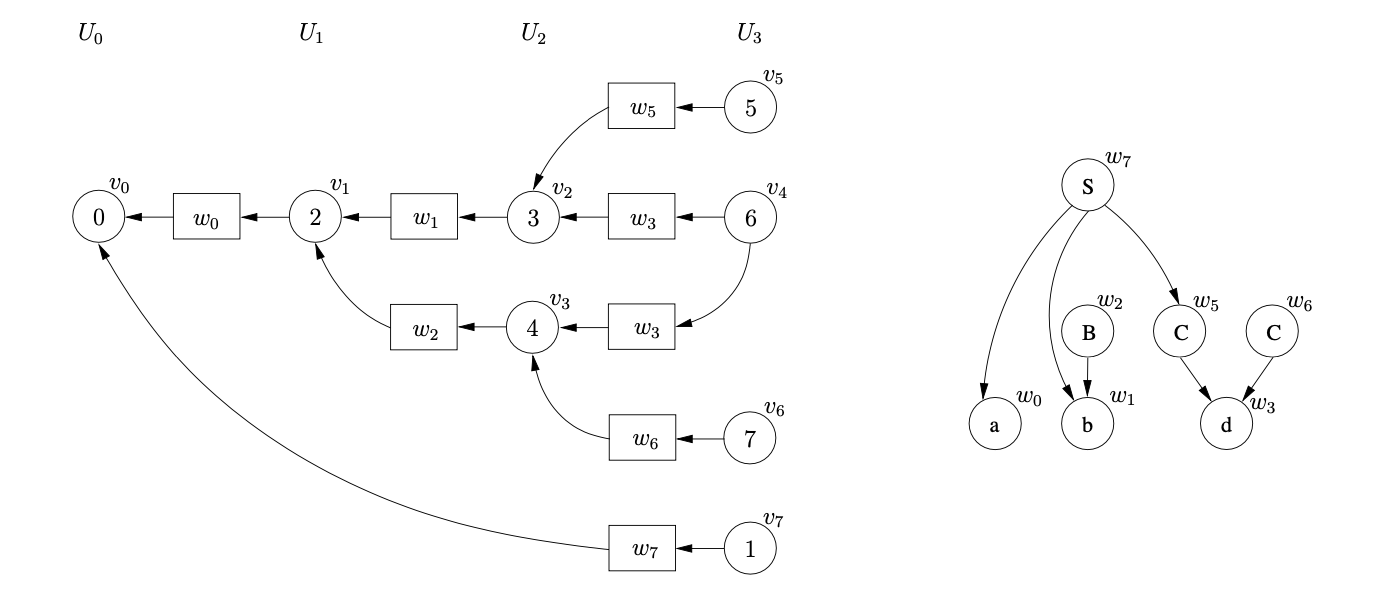
Then we process $v_{6}$ and find the reduction on rule 2, $S::=aBC$ that needs to be performed. We trace back a path of length five from $w_{6}$ to $v_{0}$ and collect the SPPF nodes $w_{2}$ and $w_{0}$. Because there is already the state node $v_{7}$ that is labelled 1, with an edge to $v_{0}$ we have encountered an ambiguity in the parse. Since the SPPF node, $w_{7}$, that is used as the symbol node on the path between $v_{7}$ and $v_{0}$ is labelled $S$ and derives the same portion of input as this reduction, we can use packing nodes below $w_{7}$ to represent both derivations.

We have parsed all the symbols on the input string and since $v_{7}$ is labelled by the accept state of the DFA, the parse terminates in success.

Although the parse was successful the final SPPF is not as compact as possible; there are still several nodes that can be shared. Since the SPPF is encoded into the symbol nodes of the GSS, sharing can only be incorporated into the SPPF if the symbol nodes are shared in the GSS. Recall that two nodes in the SPPF can be shared if the are labelled by the same symbol and have the same subtree below them.

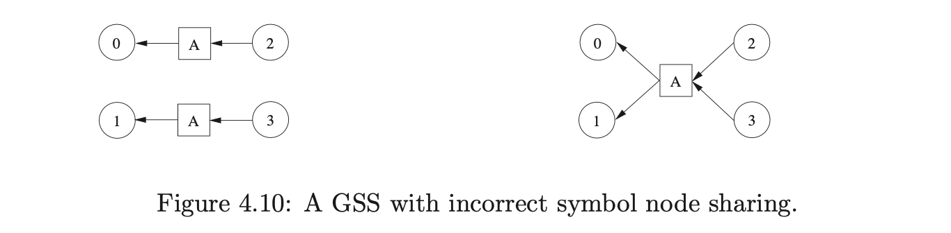
If a symbol node $v$ has a parent node in level $U_{i}$ and a child node in a level $U_{j}$ then it derives $a_{j+1}\ldots a_{i}$ of the input string $a_{1}\ldots a_{n}$[15]. Although such SPPF nodes can always be shared, it is not always possible to share the corresponding symbol node in the GSS. For example, if the two symbol nodes labelled $A$ in the GSS below are shared, then two spurious reduction paths will be introduced

Although the increased sharing of symbol nodes reduces the size of the GSS and SPPF, it comes at a cost. Before creating a new symbol node with a parent node $v$, all symbol nodes directly linked to $v$ must be searched to see if one reaches the same level as the one we want to create. So as to reduce the amount of searching performed in this way, Tomita only shares symbol nodes that are created during the same reduction. Specifically only symbol nodes that share the same reduction path up to the penultimate node are merged.

We shall now describe Rekers’ parser version of Farshi’s algorithm which generates more node sharing in the SPPF. It is this approach that we use in the RNGLR version of Tomita’s algorithm described in Chapter 5.

4.4.3 Rekers’ SPPF construction¶

It is often assumed that one of Rekers’ contributions was a correction of Tomita’s Algorithm 2. However, upon closer inspection it is clear that it is Farshi’s and not Tomita’s algorithm that forms the basis of Rekers’ parser. Rekers’ true contribution

Figure 4.10: A GSS with incorrect symbol node sharing.

is the extension of Farshi’s algorithm to a parser and the improved sharing of nodes in the SPPF.

Farshi only provides his algorithm as a recogniser, but he claims it is possible to extend it to a parser “…in a way similar to that of [Tomita]…” [11]. However, it is not straightforward to incorporate all the sharing as defined by Algorithm 3. For example, Farshi’s algorithm finds the target of a reduction path as soon as a reduction is encountered which prevents the sharing of the non-terminal symbol nodes.

In order to achieve better sharing of nodes in the SPPF Rekers does not use symbol nodes in the GSS. Instead of having a one-to-one correspondence between the GSS and SPPF, Rekers labels each of the edges in the GSS with a pointer to the associated SPPF node. This enables more nodes in the SPPF to be shared without worrying about spurious reduction paths being introduced as a result.

To achieve this sharing, it is necessary to remember the SPPF nodes that are constructed at the current step of the algorithm. Recall that nodes in the SPPF can only be shared if they are labelled by the same symbol and derive (or cover) the same portion of the input string. A naive approach to ensuring that a given node derives the same portion of the input would involve the traversal of its entire sub-tree. Rekers presents a more efficient approach that requires the SPPF nodes to be labelled by the start and end position of the string covered. This reduces the cost of the check to a comparison of the start and end positions.

Rekers’ SPPF representation contains three types of node: symbol nodes, term nodes and rule nodes. The term nodes are labelled by terminal symbols and form the leaves of the SPPF. The symbol nodes are labelled by non-terminals and have edges to rule nodes. The rule nodes are labelled by grammar rules and are equivalent to Tomita’s packing nodes. A major difference to Tomita’s representation is that every symbol node has at least one rule node as a child, even if the symbol node only has one set of children. As a result the SPPF produced by Rekers for a non-ambiguous parse is larger than that produced by Tomita.

Rekers’ parser with improved sharing in the SPPF¶

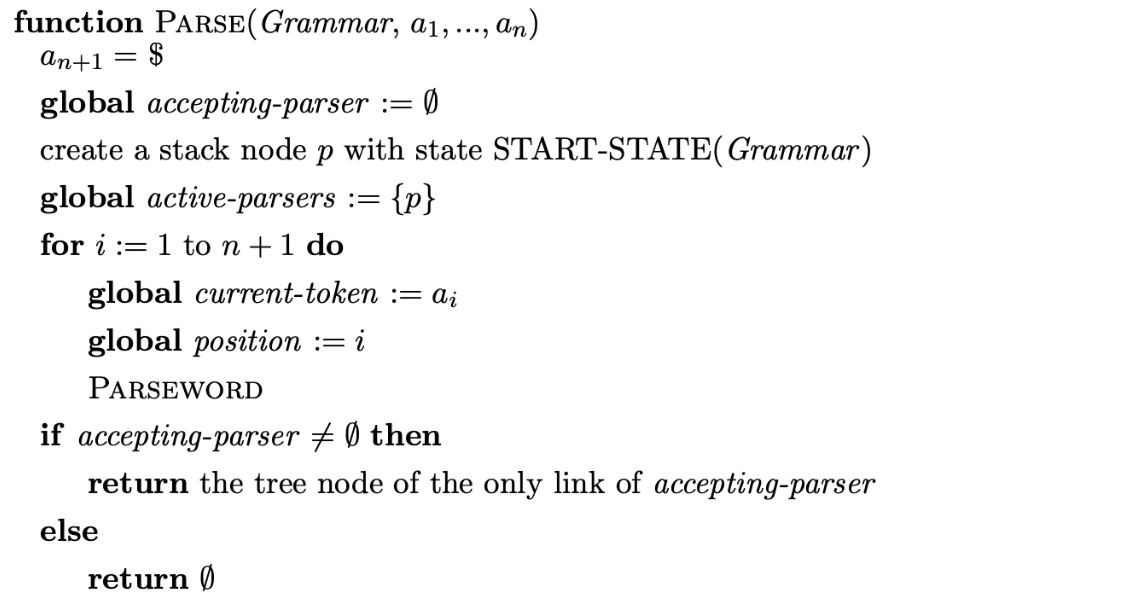
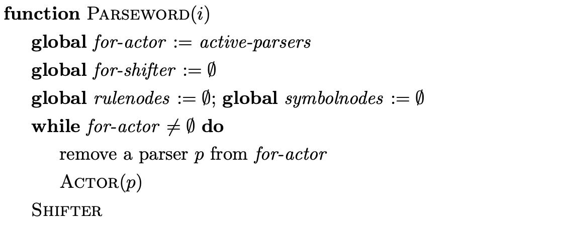
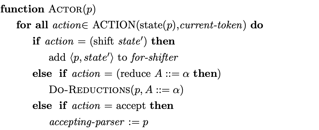
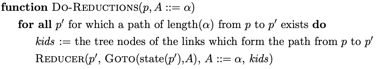
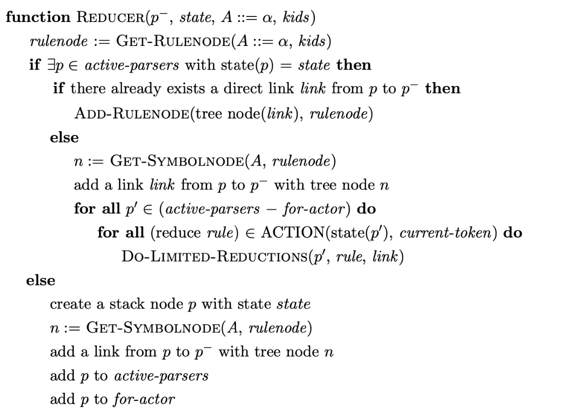
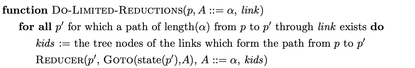
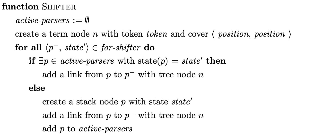
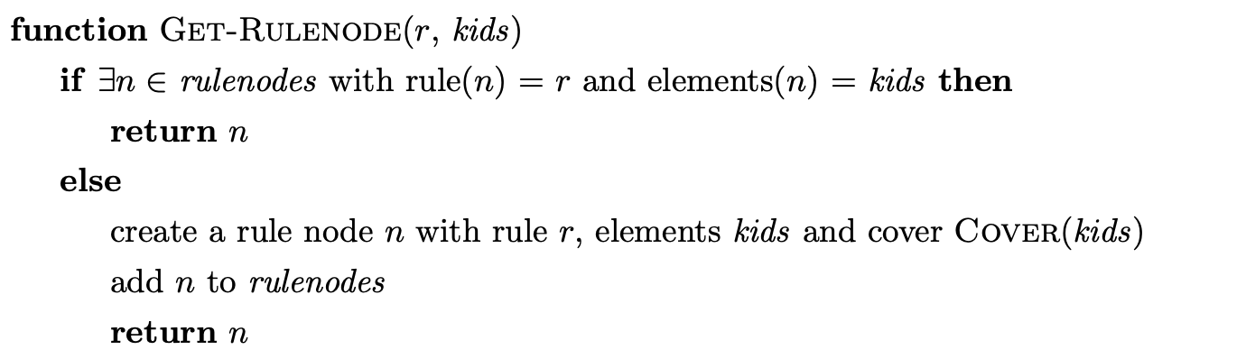
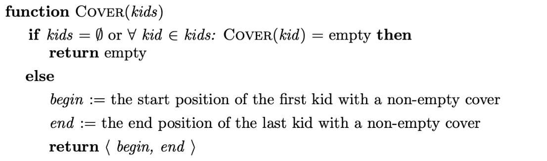
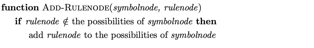
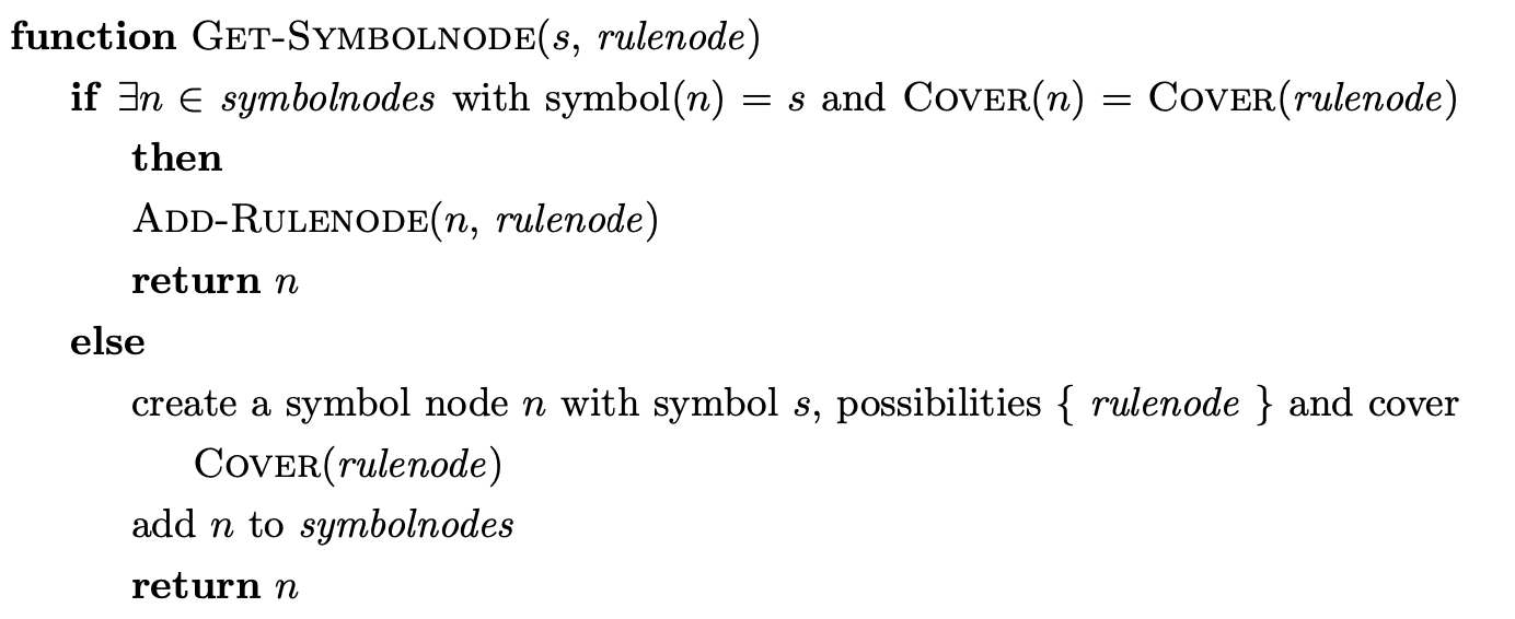
The formal description of Rekers’ parsing algorithm is taken from [10]. Although the core of Rekers’ algorithm is similar to Farshi’s, it uses slightly different notation. The sets for-actor and for-shifter are used instead of $\mathcal{A}$ and $\mathcal{Q}$ respectively and the set $\mathcal{R}$ is not used explicitly. Also, the functions Get-Rulenode, Cover, Add-Rulenode and Get-Symbolnode are added to achieve the increased sharing in the SPPF. Note that trees that derive $\epsilon$ do not cover any part of the input string. The function Cover handles this situation by always returning a non-empty position.

We demonstrate the operation of Rekers’ algorithm on the parse of the string $abd$ whose Grammar 4.1 and associated LR(1) DFA are shown on page 52.

To begin the parse we create the new state node $v_{0}$, labelled by the start state of the DFA, and add it to active-parsers. We set the current-token to $a$ and the position to 1. Then we execute the Parseword function, which leads us to copy $v_{0}$ into the for-actor and process it in the Actor function. Since there is shift to state 2 from state 0 in the DFA we add $\langle v_{0},2\rangle$ to for-shifter. We then perform the shift action in the Shifter which results in a new SPPF node $w_{0}$, labelled $a$$\langle 1,1\rangle$ being created and used to label the edge between the new node $v_{1}$ and $v_{0}$.

We continue by setting the current-token to $b$ and the position to 2 and then follow the same process as before to shift the input symbol $b$.

When we come to process $v_{2}$ in the Actor we find a shift/reduce conflict associated with state 3 on the current lookahead symbol $d$. We add $\langle v_{2},6\rangle$ to for-shifter, but before applying the shift, we perform the reduction on rule $B::=b$ by executing the Do-Reductions function.

We trace a path of length one from $v_{2}$ to $v_{1}$, collecting the SPPF node that labels the edge traversed, and then execute the Reducer function. In the Reducer we use the Get-Rulenode function to find any existing rule nodes in the SPPF that derive the same portion of the input string. Since there is none, the new rule node labelled $B::=b\ \langle 2,2\rangle$ is created. We continue by creating the new GSS node $v_{3}$ labelled $4$.

Before we create a new symbol node in the SPPF we execute the Get-Symbolnode function to ensure that a node does not already exist that can be shared. No node is found so we create the new node $w_{2}$ and use it to label the edge between $v_{3}$ and $v_{1}$.

To ensure that the new node $v_{3}$ is processed we add it to active-parsers and for-actor.

Processing $v_{3}$ in the Actor func1tion we find another shift action to state $6$. We add $\langle v_{3},6\rangle$ to for-shifter and then proceed to perform the two queued shifts in the Shifter function. This results in the creation of the new GSS node $v_{4}$ labelled $6$, with two edges back to $v_{2}$ and $v_{3}$ labelled with a pointer to the new SPPF node $w_{3}$.

Processing $v_{4}$ in the Actor function we find a reduction on rule $C::=d$. There are two different paths of length one that can be traced back from $v_{4}$ in the Do-Reductions function. For each path we collect the SPPF node that labels the edge traversed and execute the Reducer function.

In the first execution of the Reducer we create a new rule node labelled $C::=d\ \langle 3,3\rangle$ using the Get-Rulenode function and then create the new GSS node, $v_{5}$, labelled $5$. Since there does not already exist an SPPF symbol node labelled $C\ \langle 3,3\rangle$ we create $w_{4}$ and use a pointer to it to label the edge between $v_{5}$ and $v_{2}$. We also add $v_{5}$ to the active-parsers and for-actor sets.

In the second execution of the Reducer we find the rule node labelled $C::=d\ \langle 3,3\rangle$ that has the same set of children as the reduction we are performing. We create the new GSS node $v_{6}$, labelled $7$ and pass the existing rule node into the Get-Symbolnode function. However, since there is already the symbol node $w_{4}$ that is labelled by the same non-terminal and derives the same portion of the input, we do not create a new node. We use a pointer to $w_{4}$ to label the new edge between $v_{6}$ and $v_{3}$.

At this point the for-actor contains the two GSS nodes $v_{5}$ and $v_{6}$. Processing the first of the nodes we find the reduction on rule $S::=abC$. We trace back a path of length three from $v_{5}$ and collect the SPPF nodes $w_{4},w_{1},w_{0}$ that label the edges traversed. We then create a new rule node labelled $S::=abC$$\langle 1,3\rangle$ and make it the parent of the nodes previously collected. We create the new node $v_{7}$, labelled $1$, and the new symbol node $w_{5}$, labelled $S$$\langle 1,3\rangle$, as a parent of the new rule node created. We use a pointer to $w_{5}$ to label the edge between $v_{7}$ and $v_{0}$ and add $v_{7}$ to the active-parsers and for-actor sets.

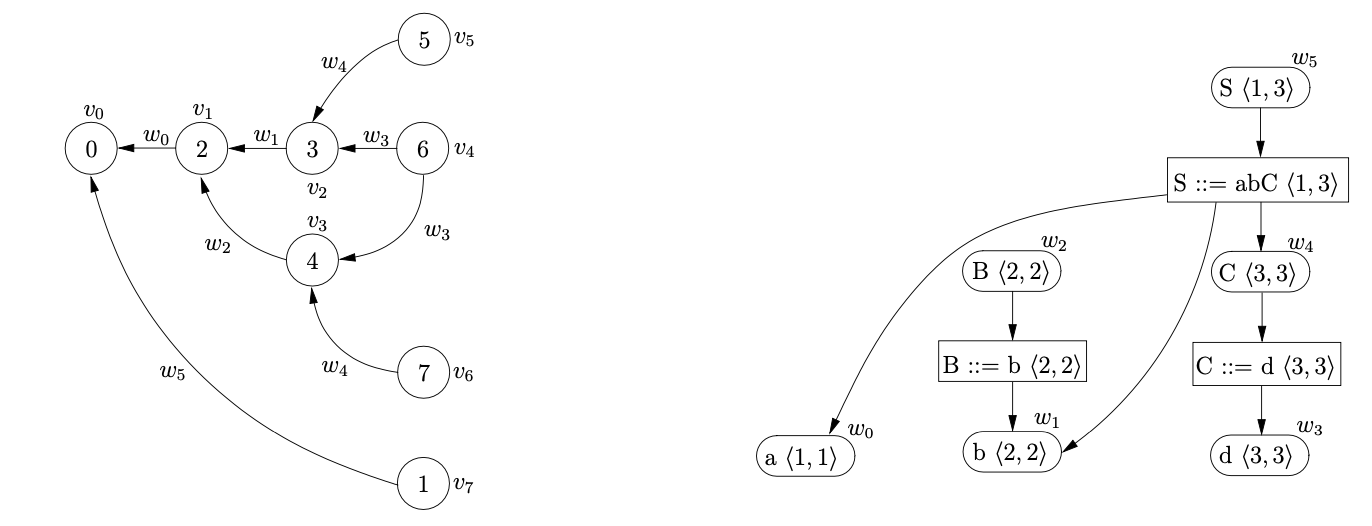
When we process $v_{6}$ we find another reduction on rule $S::=aBC$. We trace back a path of length three to $v_{0}$ and collect the SPPF nodes $w_{0},w_{2},w_{4}$ that label the edges traversed. We create the new rule node labelled $S::=aBC$$\langle 1,3\rangle$ and make it the parent of the previously collected SPPF nodes. However, we do not create a new state node in the GSS since $v_{7}$ is labelled by the goto state of the current reduction. The existence of an edge from $v_{7}$ to $v_{0}$ indicates an ambiguity in the parse. As a result we add the rule node created for this reduction as a child of $w_{5}$.

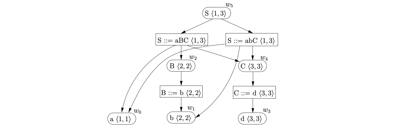
The only action associated to the state that labels $v_{7}$ is the accept action. Since all the input has been consumed the parse terminates in success and returns $w_{5}$ as the root of the SPPF.

It is clear that Rekers’ SPPF construction produces more compact SPPF’s than Tomita’s Algorithm 4. This is because Rekers’ algorithm is able to share more symbol nodes in the GSS than Tomita’s algorithm. However, to achieve this extra sharing more searching is required which causes a significant overhead in the parsing process.

4.5 Summary¶

In this chapter we have introduced Tomita’s $\text{GLR}$ parsing technique. The recognition Algorithms 1 and 2 were discussed in detail. We demonstrated the construction of the $\text{GSS}$ using Algorithm 1, and illustrated how a straightforward extension to deal with grammars containing $\epsilon$-rules fails to parse certain grammars correctly. The operation of Algorithm 2 was then examined and its non-termination for hidden-left recursive grammars was demonstrated. The extension of Algorithm 1 due to Farshi was discussed in detail and the extra costs involved were highlighted.

Finally, Tomita’s Algorithm 4 was presented that constructs an SPPF representation of multiple derivation trees and Rekers’ extension of Farshi’s algorithm was introduced.

Chapter 10 presents the experimental results of a naive and optimised implementation of Farshi’s recogniser for grammars which trigger worst case behaviour and several programming language grammars and strings.

The next chapter presents the $\text{RNGLR}$ algorithm that correctly parses all context-free grammars using a modified $\text{LR}$ parse table. The $\text{RNGLR}$ parser incorporates some of Rekers’ sharing into the $\text{SPPF}$, but reduces the amount of searching required.