Perface

CHANGES IN THE THIRD EDITION

The changes introduced in the third edition of Engineering a Com- piler (EaC3e) arise from two principal sources: changes in the way that programming-language translation technology is used and changes in the technical backgrounds of our students. These two driving forces have led to continual revision in the way that we teach compiler construction. This third edition captures those classroom-tested changes.

EaC3e reorganizes the material, discarding some topics from prior editions and introducing some topics that are new—at least in this book. EaC2e included major changes to the material on optimization (Chapters 8, 9, and 10); those chapters are largely intact from the second edition. For EaC3e, we have made changes throughout the book, with a particular focus on re- organization and revision in the middle of the book: Chapters 4 through 7. The widespread use of just-in-time (JIT) compilers prompted us to add a chapter to introduce these techniques. In terms of specific content changes:

The chapter on intermediate representations now appears as Chapter 4, before syntax-driven translation. Students should be familiar with that material before they read about syntax-driven translation.
The material on attribute grammars that appeared in Chapter 4 of the first two editions is gone. Attribute grammars are still an interesting topic, but it is clear that ad-hoc translation is the dominant paradigm for translation in a compiler’s front end.
Chapter 5 now provides a deeper coverage of both the mechanism of syntax-driven translation and its use. Several translation-related topics that were spread between Chapters 4, 6, and 7 have been pulled into this new chapter.
Chapter 7 has a new organization and structure, based on extensive in- class experimentation.

Earlier editions called Best’s algorithm the “bottom-up local” algorithm.

Chapter 13 now focuses on two allocators: a local allocator based on Best’s algorithm and a global allocator based on the work of Chaitin and Briggs. The Advanced Topics section of Chapter 13 explores modifica- tions of the basic Chaitin-Briggs scheme that produce techniques such as linear scan allocators, SSA-based allocators, and iterative coalescing allocators.
Chapter 14 provides an overview of runtime optimization or JIT- compilation. JIT compilers have become ubiquitous. Students should understand how JIT compilers work and how they relate to classic ahead-of-time compilers.

Our goal continues to be a text and a course that expose students to critical issues in modern compilers and provide them with the background to tackle those problems.

We usually omit Chapters 9 and 10 in the undergraduate course. Chapter 14 elicits, in our experience, more student interest.

ORGANIZATION

EaC3e divides the material into four roughly equal pieces:

■ The first section, Chapters 2 and 3, covers the design of a compiler’s front end and the algorithms that go into tools that automate front-end construction. In teaching the algorithms to derive scanners from regular expressions and parsers from context-free grammars, the text introduces several key concepts, including the notion of a fixed-point algorithm.

■ The second section, Chapters 4 through 7, explores the mapping of source code into the compiler’s intermediate form. These chapters ex- amine the kinds of code that the front end can generate for the optimizer and the back end.

We usually omit Chapters 9 and 10 in the undergraduate course. Chapter 14 elicits, in our experience, more student interest.

■ The third section, Chapters 8, 9, 10, and 14, presents an overview of code optimization. Chapter 8 provides a broad look at the kinds of op- timization that compilers perform. Chapters 9 and 10 dive more deeply into data-flow analysis and scalar optimization. Chapter 14 fits themati- cally into this section; it assumes knowledge of the material in the fourth section.

■ The fourth section, Chapters 11 through 13, focuses on the major algo- rithms found in a compiler’s back end: instruction selection, instruction scheduling, and register allocation. In the third edition, we have revised the material on register allocation so that it focuses on fewer ideas and covers them at greater depth. The new chapter provides students with a solid basis for understanding most of the modern allocation algo- rithms.

Our undergraduate course takes a largely linear walk through this material. We often omit Chapters 9 and 10 due to a lack of time. The material in Chapter 14 was developed in response to questions from students in the course.

APPROACH

Compiler construction is an exercise in engineering design. The compiler writer must choose a path through a design space that is filled with di- verse alternatives, each with distinct costs, advantages, and complexity. Each decision has an impact on the resulting compiler. The quality of the end product depends on informed decisions at each step along the way.

Thus, there is no single right answer for many of the design decisions in a compiler. Even within “well-understood” and “solved” problems, nuances in design and implementation have an impact on both the behavior of the compiler and the quality of the code that it produces. Many considerations play into each decision. As an example, the choice of an intermediate repre- sentation for the compiler has a profound impact on the rest of the compiler, from time and space requirements through the ease with which different al- gorithms can be applied. The decision, however, is often given short shrift. Chapter 4 examines the space of intermediate representations and some of the issues that should be considered in selecting one. We raise the issue again at several points in the book—both directly in the text and indirectly in the exercises.

EaC3e explores the compiler construction design space and conveys both the depth of problems and the breadth of the possible solutions. It presents some of the ways that problems in compilation have been solved, along with the constraints that made those solutions attractive. Compiler writers need to understand both the parameters of the problems and their solutions. They must recognize that a solution to one problem can affect both the opportu- nities and constraints that appear in other parts of the compiler. Only then can they make informed and intelligent design choices.

PHILOSOPHY

This text exposes our philosophy for building compilers, developed during more than forty years each of research, teaching, and practice. For example, intermediate representations should expose those details that matter in the final code; this belief leads to a bias toward low-level representations. Val- ues should reside in registers until the allocator discovers that it cannot keep them there; this practice leads to compilers that operate in terms of virtual registers and that only store values to memory when it cannot be avoided. This approach also increases the importance of effective algorithms in the compiler’s back end. Every compiler should include optimization; it simpli- fies the rest of the compiler. Our experiences over the years have informed the selection of material and its presentation.

A WORD ABOUT PROGRAMMING EXERCISES

A class in compiler construction offers the opportunity to explore complex problems in the context of a concrete application—one whose basic func- tions are well understood by any student with the background for a compiler construction course. In most versions of this course, the programming exer- cises play a large role.

We have taught this class in versions where the students build a simple com- piler from start to finish—beginning with a generated scanner and parser and ending with a code generator for some simplified RISC instruction set. We have taught this class in versions where the students write programs that address well-contained individual problems, such as register allocation or instruction scheduling. The choice of programming exercises depends heavily on the role that the course plays in the surrounding curriculum.

In some schools, the compiler course serves as a capstone course for seniors, tying together concepts from many other courses in a large, practical, design and implementation project. Students in such a class might write a complete compiler for a simple language or modify an open-source compiler to add support for a new language feature or a new architectural feature. This ver- sion of the class might present the material in a linear order that closely follows the text’s organization.

In some schools, that capstone experience occurs in other courses or in other ways. In this situation, the teacher might focus the programming exercises more narrowly on algorithms and their implementations, using labs such as a local register allocator or a tree-height rebalancing pass. This version of the course might skip around in the text and adjust the order of presenta- tion to meet the needs of the labs. We have found that students entering the course understand assembly-language programming, so they have no prob- lem understanding how a scheduler or a register allocator should work.

In either scenario, the course should make connections to other classes in the undergraduate curriculum. The course has obvious ties to computer or- ganization, assembly-language programming, operating systems, computer architecture, algorithms, and formal languages. Less obvious connections abound. The material in Chapter 7 on character copying raises performance issues that are critical in protocol-stack implementation. The material in Chapter 2 has applications that range from URL-filtering through specify- ing rules for firewalls and routers. And, of course, Best’s algorithm from Chapter 13 is an earlier version of Belady’s offline page replacement algo- rithm, MIN.

ADDITIONAL MATERIALS

Additional resources are available to help you adapt the material pre- sented in EaC3e to your course. These include a complete set of slides from the authors’ version of the course at Rice University and a set of solutions to the exercises. Visit https://educate.elsevier.com/book/details/ 9780128154120 for more information.

ACKNOWLEDGMENTS

Many people were involved in the preparation of this third edition of Engi- neering a Compiler. People throughout the community have gently pointed out inconsistencies, typographical problems, and errors. We are grateful to each of them.

Teaching is often its own reward. Two colleagues of ours from the class- room, Zoran Budimlic ́ and Michael Burke, deserve special thanks. Zoran is a genius at thinking about how to abstract a problem. Michael has deep insights into the theory behind both the front-end section of the book and the optimization section. Each of them has influenced the way that we think about some of this material.

The production team at Elsevier, specifically Beth LoGiudice, Steve Merken, and Manchu Mohan, played a critical role in the conversion of a rough manuscript into its final form. All of these people improved this volume in significant ways with their insights and their help. Aaron Keen, Michael Lam, and other reviewers provided us with valuable and timely feedback on Chapter 14.

Finally, many people have provided us with intellectual and emotional sup- port over the last five years. First and foremost, our families and our col- leagues at Rice have encouraged us at every step of the way. Christine and Carolyn, in particular, tolerated myriad long discussions on topics in compiler construction. Steve Merken guided this edition from its inception through its publication with enthusiasm, extreme patience, and good humor. To all these people go our heartfelt thanks.

Chapter 4 Intermediate Representations

ABSTRACT

The central data structure in a compiler is its representation of the program being compiled. Most passes in the compiler read and manipulate this intermediate representation or IR. Thus, decisions about what to represent and how to represent it play a crucial role in both the cost of compilation and its effectiveness. This chapter presents a survey of IRs that compilers use, including graphical IRs, linear IRs, and hybrids of these two forms, along with the ancillary data structures that the compiler maintains, typified by its symbol tables.

KEYWORDS

Intermediate Representation, Graphical IR, Linear IR, SSA Form, Symbol Table, Memory Model, Storage Layout

4.1 Introduction

Compilers are typically organized as a series of passes. As the compiler derives knowledge about the code it translates, it must record that knowledge and convey it to subsequent passes. Thus, the compiler needs a representation for all of the facts that it derives about the program. We call this collection of data structures an intermediate representation (IR). A compiler may have one IR, or it may have a series of IRs that it uses as it translates from the source code into the target language. The compiler relies on the IR to represent the program; it does not refer back to the source text. The properties of the IR have a direct effect on what the compiler can and cannot do to the code.

Use of an IR lets the compiler make multiple passes over the code. The compiler can generate more efficient code for the input program if it can gather information in one pass and use it in another. However, this capability imposes a requirement: the IR must be able to represent the derived information. Thus, compilers also build a variety of ancillary data structures to represent derived information and provide efficient access to it. These structures also form part of the IR.

Almost every phase of the compiler manipulates the program in its IR form. Thus, the properties of the IR, such as the methods for reading and writing specific fields, for finding specific facts, and for navigating around the program, have a direct impact on the ease of writing the individual passes and on the cost of executing those passes.

Conceptual Roadmap

This chapter focuses on the issues that surround the design and use of IRs in compilation. Some compilers use trees and graphs to represent the program being compiled. For example, parse trees easily capture the derivations built by a parser and Lisp's S-expressions are, themselves, simple graphs. Because most processors rely on a linear assembly language, compilers often use linear IRs that resemble assembly code. Such a linear IR can expose properties of the target machine's native code that provide opportunities to the compiler.

As the compiler builds up the IR form of the program, it discovers and derives information that may not fit easily into a tree, graph, or linear IR. It must understand the name space of the program and build ancillary structures to record that derived knowledge. It must create a plan for the layout of storage so that the compiled code can store values into memory and retrieve them as needed. Finally, it needs efficient access, by name, to all of its derived information. To accommodate these needs, compilers build a set of ancillary structures that coexist with the tree, graph, or linear IR and form a critical part of the compiler's knowledge base about the program.

Overview

Modern multipass compilers use some form of IR to model the code being analyzed, translated, and optimized. Most passes in the compiler consume IR; the stream of categorized words produced by the scanner can be viewed as an IR designed to communicate between the scanner and the parser. Most passes in the compiler produce IR; passes in the code generator can be exceptions. Many modern compilers use multiple IRs during the course of a single compilation. In a pass-structured compiler, the IR serves as the primary representation of the code.

A compiler's IR must be expressive enough to record all of the useful facts that the compiler might need to transmit between passes. Source code is insufficient for this purpose; the compiler derives many facts that have no representation in source code. Examples include the addresses of variables or the register number in which a given parameter is passed. To record all of the details that the compiler must encode, most compiler writers augment the IR with tables and sets that record additional information. These structures form an integral part of the IR.

Selecting an appropriate IR for a compiler project requires an understanding of the source language, the target machine, the goals for the compiler, and the properties of the applications that the compiler will translate. For example, a source-to-source translator might use a parse tree that closely resembles the source code, while a compiler that produces assembly code for a microcontroller might obtain better results with a low-level assembly-like IR. Similarly, a compiler for C might need annotations about pointer values that are irrelevant in a LISP compiler. Compilers for JAVA or C++ record facts about the class hierarchy that have no counterpart in a C compiler.

Common operations should be inexpensive. Uncommon operations should be doable at a reasonable cost.

For example, ILOC's $\Rightarrow$ symbol has one purpose: to improve readability.

Implementing an IR forces the compiler writer to focus on practical issues. The IR is the compiler's central data structure. The compiler needs inexpensive ways to perform the operations that it does frequently. It needs concise ways to express the full range of constructs that might arise during compilation. Finally, the compiler writer needs mechanisms that let humans examine the IR program easily and directly; self-interest should ensure that compiler writers pay heed to this last point.

The remainder of this chapter explores the issues that arise in the design and use of IRs. Section 4.2 provides a taxonomy of IRs and their properties. Section 4.3 describes several IRs based on trees and graphs, while Section 4.4 presents several common linear forms of IRs. Section 4.5 provides a high-level overview of symbol tables and their uses; Appendix B.4 delves into some low-level hash-table implementation issues. The final two sections, 4.6 and 4.7, explore issues that arise from the way that the compiler names values and the rules that the compiler applies to place values in memory.

A Few Words About Time

Intermediate representations are, almost entirely, a compile-time construct. Thus, the compiler writer has control over the IR design choices, which she makes at design time. The IR itself is instantiated, used, and discarded at compile time.

Some of the ancillary information generated as part of the IR, such as symbol tables and storage maps, is preserved for later tools, such as the debugger. Those use cases, however, do not affect the design and implementation of the IR because that information must be translated into some standard form dictated by the tools.

4.2 An ir taxonomy

Compilers have used many kinds of ir. We will organize our discussion of ir along three axes: structural organization, level of abstraction, and mode of use. In general, these three attributes are independent; most combinations of organization, abstraction, and naming have been used in some compiler.

Structural Organization

Broadly speaking, irs fall into three classes:

Graphical IRs: encode the compiler's knowledge in a graph. Algorithms then operate over nodes and edges. The parse trees used to depict derivations in Chapter 3 are an instance of a graphical ir, as are the trees shown in panels (a) and (c) of Fig. 4.1. Linear IRs: resemble pseudocode for some abstract machine. The algorithms iterate over simple, linear sequences of operations. The ILOC code used in this book is a form of linear ir, as are the representations shown in panels (b) and (d) of Fig. 4.1.

Compiler writers use the acronym CFG for both context-free grammar and control-flow graph. The difference should be clear from context.

Hybrid IRs: combine elements of both graphical and linear ir, to capture their strengths and avoid their weaknesses. A typical control-flow graph (CFG) uses a linear ir to represent blocks of code and a graph to represent the flow of control among those blocks.

The structural organization of an ir has a strong impact on how the compiler writer thinks about analysis, optimization, and code generation. For example, tree-structured ir lead naturally to passes organized as some form of treewalk. Similarly, linear ir lead naturally to passes that iterate over the operations in order.

Level of Abstraction

The compiler writer must also choose the level of detail that the ir will expose: its level of abstraction. The ir can range from a near-source form in which a couple of nodes represent an array access or a procedure call to a low-level form in which multiple ir operations must be combined to form a single target-machine operation. To illustrate the possibilities, the drawing in the margin shows a reference to a[i,j] represented in a source-level tree. Below it, the same reference is shown in ILOC. In both cases, a is a $10 \times 10$ array of 4-byte elements.

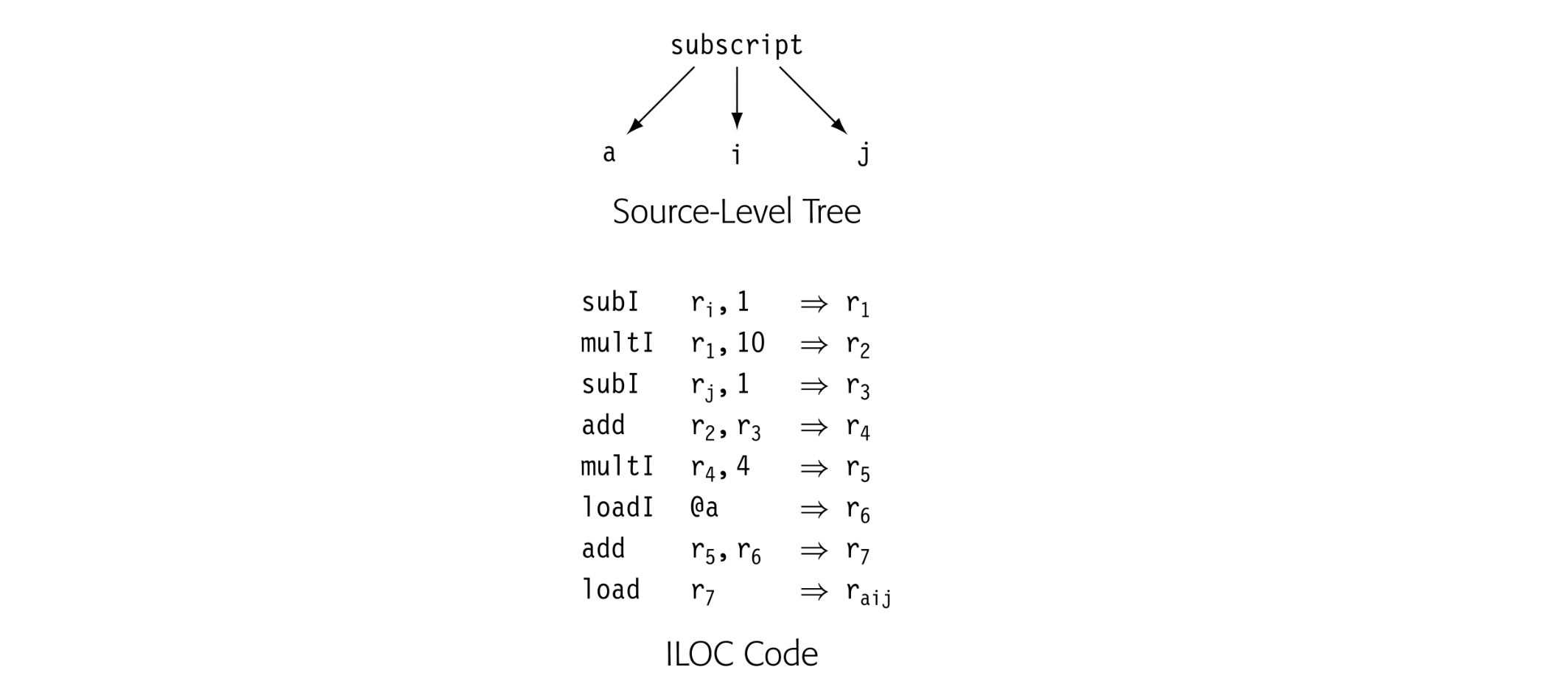
In the source-level tree, the compiler can easily recognize the computation as an array reference, whereas the ILOC code obscures that fact fairly well. In a compiler that tries to determine when two different references can touchthe same memory location, the source-level tree makes it easy to find and compare references. By contrast, the ILOC code makes those tasks hard. On the other hand, if the goal is to optimize the final code generated for the array access, the ILOC code lets the compiler optimize details that remain implicit in the source-level tree. For this purpose, a low-level IR may prove better.

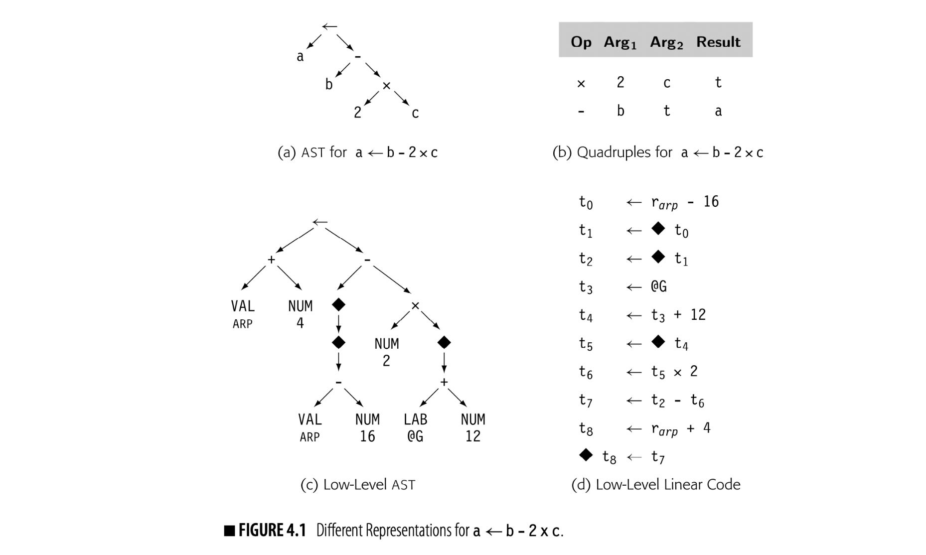
Level of abstraction is independent of structure. Fig. 4.1 shows four different representations for the statement a $\leftarrow$ b - 2 x c. Panels (a) and (c) show abstract syntax trees (ASTs) at both a near-source level and a near-machine level of abstraction. Panels (b) and (d) show corresponding linear representations.

The translation of $⧫$ in the low-level linear code depends on context. To the left of a $\leftarrow$ operator, it represents a store. To the right, it represents a load.

The low-level AST in panel (c) uses nodes that represent assembly-level concepts. A VAL node represents a value already in a register. A NUM node represents a known constant that can fit in an operation's immediate field. A LAB node represents an assembly-level label. The dereference operator, $⧫$ , treats the value as an address and represents a memory reference. This particular AST will reappear in Chapter 11.

Level of abstraction matters because the compiler can, in general, only optimize details that the IR exposes. Facts that are implicit in the IR are hard to change because the compiler treats implicit knowledge in uniform ways, which mitigates against context-specific customization. For example, to optimize the code for an array reference, the compiler must rewrite the IR for the reference. If the details of that reference are implicit, the compiler cannot change them.

Mode of Use

The third axis relates to the way that the compiler uses an IR.

A definitive IR is the primary representation for the code being compiled. The compiler does not refer back to the source code; instead, it analyzes, transforms, and translates one or more (successive) IR versions of the code. These IRs are definitive IRs.
A derivative IR is one that the compiler builds for a specific, temporary purpose. The derivative IR may augment the definitive IR, as with a dependence graph for instruction scheduling (see Chapter 12). The compiler may translate the code into and out of the derivative IR to enable a specific optimization.

In general, if an IR is transmitted from one pass to another, it should be considered definitive. If the IR is built within a pass for a specific purpose and then discarded, it is derivative.

Naming

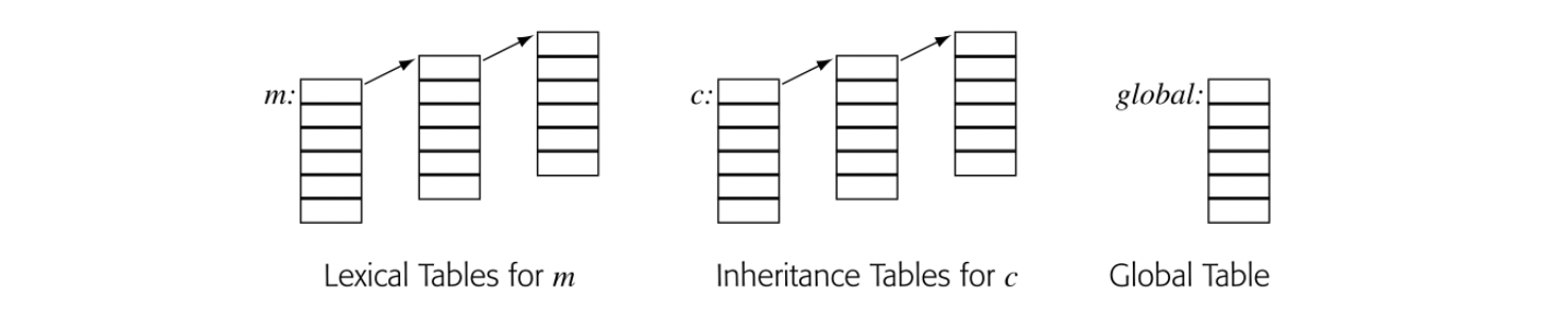
The compiler writer must also select a name space for the IR. This decision will determine which values in the program are exposed to optimization. As it translates the source code, the compiler must choose names and storage locations for myriad distinct values.

Fig. 4.1 makes this concrete. In the ASTs, the names are implicit; the compiler can refer to any subtree in the AST by the node that roots the subtree. Thus, the tree in panel (c) names many values that cannot be named in panel (a), because of its lower level of abstraction. The same effect occurs in the linear codes. The code in panel (b) creates just two values that other operations can use while the code in panel (d) creates nine.

The naming scheme has a strong effect on how optimization can improve the code. In panel (d), t0 is the runtime address of b, t4 is the runtime address of c, and t8 is the runtime address of a. If nearby code references any of these locations, optimization should recognize the identical references and reuse the computed values (see Section 8.4.1). If the compiler reused the name t0 for another value, the computed address of b would be lost, because it could not be named.

REPRESENTING STRINGS

The scanner classifies words in the input program into a small set of categories. From a functional perspective, each word in the input stream becomes a pair ⟨ lexeme, category ⟩, where lexeme is the word’s text and category is its syntactic category. > For some categories, having both lexeme and category is redundant. The categories +, ×, and for have only one lexeme. For others, such as identifiers, numbers, and character strings, distinct words have distinct lexemes. For these categories, the compiler will need to represent and compare the lexemes. > >Character strings are one of the least efficient ways that the compiler can represent a name. The character string’s size is proportional to its length. To compare two strings takes, in general, time proportional to their length. A compiler can do better. >

The compiler should, instead, map the names used in the original code into a compact set of integers. This approach saves space; integers are denser than character strings. This approach saves time; comparisons for equality take $O (1)$ time.

To accomplish this mapping, the compiler writer can have the scanner create a hash table (see Appendix B.4) to hold all the distinct strings used in the input program. Then the compiler can use either the string’s index in this “string table” or a pointer to its record in the string table as a proxy for the string. Information derived from the string, such as the length of a string constant or the value and type of a numerical constant, can be computed once and referenced quickly through the table.

Using too few names can undermine optimization. Using too many can bloat some of the compile-time data structures and increase compile time without benefit. Section 4.6 delves into these issues.

Practical Considerations

As a practical matter, the costs of generating and manipulating an IR should concern the compiler writer, since they directly affect a compiler's speed. The data-space requirements of different IRs vary over a wide range. Since the compiler typically touches all of the space that it allocates, data space usually has a direct relationship to running time.

Last, and certainly not least, the compiler writer should consider the expressiveness of the IR--its ability to accommodate all the facts that the compiler needs to record. The IR for a procedure might include the code that defines it, the results of static analysis, profile data from previous executions, andmaps to let the debugger understand the code and its data. All of these facts should be expressed in a way that makes clear their relationship to specific points in the IR.

4.3 Graphical Irs

Many compilers use IRs that represent the underlying code as a graph. While all the graphical IRs consist of nodes and edges, they differ in their level of abstraction, in the relationship between the graph and the underlying code, and in the structure of the graph.

Parse trees, ASTs, and directed acyclic graphs (DAGs) are all graphs used to represent code. These tree-like IRs have a structure that corresponds to the syntax of the source code.

Parse Trees

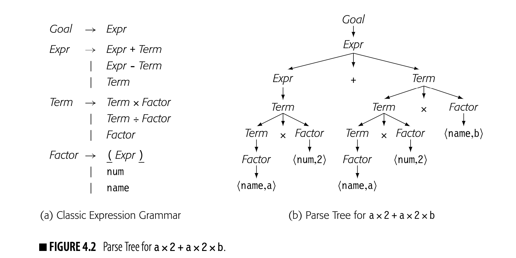
As we saw in Section 3.2, the parse tree is a graphical representation for the derivation, or parse, of the input program. Fig. 4.2 shows the classic expression grammar alongside a parse tree for $a \times 2 + a \times 2 \times b$ . The parse tree is large relative to the source text because it represents the complete derivation, with a node for each grammar symbol in the derivation. Since the compiler must allocate memory for each node and each edge, and it must traverse all those nodes and edges during compilation, it is worth considering ways to shrink this parse tree.

Minor transformations on the grammar, as described in Section 3.6.1, can eliminate some of the steps in the derivation and their corresponding parse-tree nodes. A more effective way to shrink the parse tree is to abstract away those nodes that serve no real purpose in the rest of the compiler. This approach leads to a simplified version of the parse tree, called an abstract syntax tree, discussed below.

Mode of Use: Parse trees are used primarily in discussions of parsing, and in attribute-grammar systems, where they are the definitive ir. In most other applications in which a source-level tree is needed, compiler writers tend to use one of the more concise alternatives, such as an ast or a dag.

Abstract Syntax Trees

Abstract syntax tree a contraction of the parse tree that omits nodes for most nonterminals

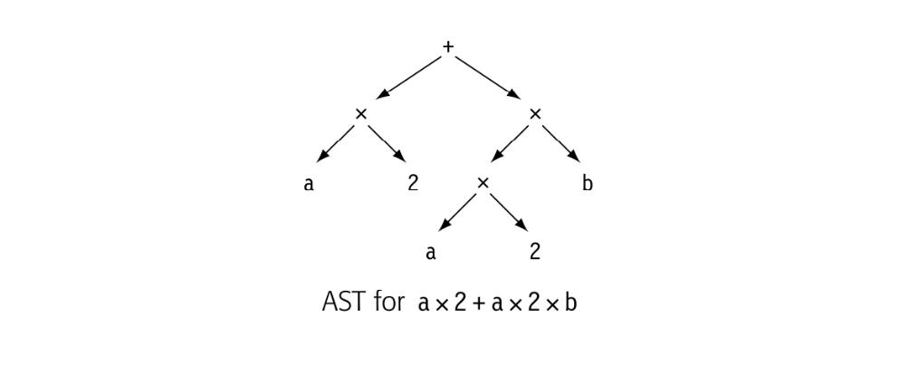
The abstract syntax tree (AST) retains the structure and meaning of the parse tree but eliminates extraneous nodes. It eliminates the nodes for non-terminal symbols that encode the details of the derivation. An ast for a x 2 + a x 2 $\times$ b is shown in the margin.

Mode of Use: ASTs have been used as the definitive ir in many practical compiler systems. The level of abstraction that those systems need varies widely.

Source-to-source systems, including syntax-directed editors, code-refactoring tools, and automatic parallelization systems, often use an ast with near-source abstractions. The structure of a near-source ast reflects the structure of the input program.
Compilers that generate assembly code may use an ast. These systems typically start with a near-source ast and systematically lower the level of abstraction until it is at or below the abstraction level of the target machine's isa. The structure of that final, low-level ast tends to reflect the flow of values between operations.

Ast-based systems usually use treewalks to traverse the ir. Many of the algorithms used in compilation have natural formulations as either a treewalk (see Section 11.4) or a depth-first search (see Section 8.5.1).

Some compilers build asts as derivative ir because conversion into and out of an ast is fast and because it may simplify other algorithms. In particular, optimizations that rearrange expressions benefit from building an ast as a derivative ir because the ast eliminates all of the explicit names for intermediate results. Other algorithms, such as tree-height balancing (Section 8.4.2) or tree-pattern matching (Section 11.4) have "natural" expressions as tree traversals.

CHOOSING THE RIGHT ABSTRACTION

Even with a source level tree, representation choices affect usability. For example, the Rn Programming Environment used the subtree shown in panel (a) below to represent a complex number in FORTRAN, which was written as (c1,c2). This choice worked well for the syntax-directed editor, in which the programmer was able to change c1 and c2 independently; the pair node corresponded to the parentheses and the comma. The pair format, however, proved problematic for the compiler. Each part of the compiler that dealt with constants needed special-case code for complex constants.

All other constants were represented with a single node that contained a pointer to the constant’s lexeme, as shown above in panel (b). Using a similar format for complex constants would have complicated the editor, but simplified the compiler. Taken over the entire system, the benefits would likely have outweighed the complications.

Directed Acyclic Graphs

Directed acyclic graph A DAG is an AST that represents each unique subtree once. DAGs are often called ASTs with sharing.

While an AST is more concise than a parse tree, it faithfully retains the structure of the original source code. For example, the AST for a x 2+ a x 2 x b contains two distinct copies of the expression a x 2. A directed acyclic graph (DAG) is a contraction of the AST that avoids this duplication. In a DAG, nodes can have multiple parents, and identical subtrees are reused. Such sharing makes the DAG more compact than the corresponding AST.

For expressions without assignment or function calls, textually identical expressions must produce identical values. The DAG for $a \times 2 + a \times 2 \times b$ , shown in the margin, reflects this fact by sharing a single copy of a x 2. If the value of a cannot change between the two uses of a, then the compiler should generate code to evaluate $a \times 2$ once and use the result twice. This strategy can reduce the cost of evaluation. The DAG explicitly encodes the redundancy among subexpressions. If the compiler represents such facts in the ir, it can avoid the costs of rediscovering them.

When building the DAG for this expression, the compiler must prove that a's value cannot change between uses. If the expression contains neither assignments nor calls to other procedures, the proof is easy. Since an assignment or a procedure call can change the value associated with a name, the DAG construction algorithm must invalidate subtrees when the values of their operands can change.

STORAGE EFFICIENCY AND GRAPHICAL REPRESENTATIONS

Many practical systems have used abstract syntax trees as their definitive IR. Many of these systems found that the AST was large relative to the size of the input text. In the $R^{n}$ Programming Environment built at Rice in the 1980s, AST size posed two problems: mid-1980s workstations had limited memory, and tree-l/O slowed down all of the $R^{n}$ tools.

$R^{n}$ AST nodes used 92 bytes. The IR averaged 11 nodes per sourcelanguage statement. Thus, the AST needed about 1,000 bytes per statement. On a 4MB workstation, this imposed a practical limit of about 1,000 lines of code in most of the environment's tools.

No single decision led to this problem. To simplify memory allocation, $R^{n}$ ASTs had only one kind of node. Thus, each node included all the fields needed by any node. (Roughly half the nodes were leaves, which need no pointers to children.) As the system grew, so did the nodes. New tools needed new fields.

Careful attention can combat this kind of node bloat. In $R^{n}$ , we built programs to analyze the contents of the AST and how it was used. We combined some fields and eliminated others. (In some cases, it was cheaper to recompute information than to write it and read it.) We used hash-linking to move rarely used fields out of the AST and into an ancillary table. (One bit in the node-type field indicated the presence of ancillary facts related to the node.) For disk I/O, we converted the AST to a linear form in a preorder treewalk, which made pointers implicit.

In $R^{n}$ , these changes reduced the size of ASTs in memory by about 75 percent. On disk, the files were about half the size of their memory representation. These changes let $R^{n}$ handle larger programs and made the tools noticeably more responsive.

Mode of Use: DAGs are used in real systems for two primary reasons. If memory constraints limit the size of programs that the compiler can process, using a DAG as the definitive IR can reduce the IR's memory footprint. Other systems use DAGs to expose redundancies. Here, the benefit lies in better compiled code. These latter systems tend to use the DAG as a derivative IR--build the DAG, transform the definitive IR to reflect the redundancies, and discard the DAG.

4.3.2 Graphs

While trees provide a natural representation for the grammatical structure that parsing discovers in the source code, their rigid structure makes them less useful for representing other properties of programs. To model these aspects of program behavior, compilers often use more general graphs as Its. The DAG introduced in the previous section is one example of a graph.

Control-Flow Graph

Basic block a maximal length sequence of branch-free code

The simplest unit of control flow is a basic block--a maximal length sequence of straight-line, or branch-free, code. The operations in a block always execute together, unless some operation raises an exception. A block begins with a labeled operation and ends with a branch, jump, or predicated operation. Control enters a basic block at its first operation. The operations execute in an order consistent with top-to-bottom order in the block. Control exits at the block's last operation.

Control-flow graph A CFG has a node for each basic block and an edge for each possible transfer of control.

A control-flow graph (CFG) models the flow of control between the basic blocks in a procedure. A CFG is a directed graph, $G = (N$ , $E)$ . Each node $n \in N$ corresponds to a basic block. Each edge $e = (n_{i}, n_{j}) \in E$ corresponds to a possible transfer of control from block $n_{i}$ to block $n_{j}$ .

If the compiler adds artificial entry and exit nodes, they may not correspond to actual basic blocks.

To simplify the discussion of program analysis in Chapters 8 and 9, we assume that each CFG has a unique entry node, $n_{0}$ , and a unique exit node, $n_{f}$ . If a procedure has multiple entries, the compiler can create a unique $n_{0}$ and add edges from $n_{0}$ to each actual entry point. Similarly, $n_{f}$ corresponds to the procedure's exit. Multiple exits are more common than multiple entries, but the compiler can easily add a unique $n_{f}$ and connect each of the actual exits to it.

The CFG provides a graphical representation of the possible runtime control-flow paths. It differs from syntax-oriented Its, such as an AST, which show grammatical structure. Consider the while loop shown below. Its CFG is shown in the center pane and its AST in the rightmost pane.

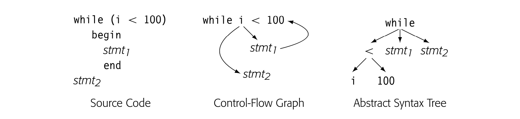
The CFG captures the essence of the loop: it is a control-flow construct. The cyclic edge runs from $stm t_{l}$ back to the test at the head of the loop. Bycontrast, the AST captures the syntax; it is acyclic but puts all the pieces in place to regenerate the source-code for the loop.

For an if-then-else construct both the CFG and the AST would be acyclic, as shown below. 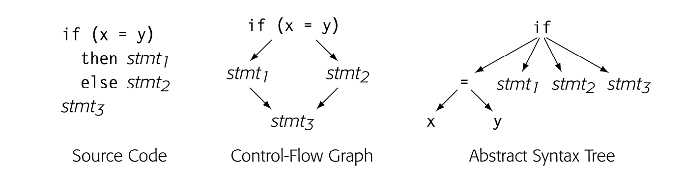Again, the CFG models the control flow; one of stmt1 or stmt2 executes, but not both of them. The AST again captures the syntax but provides little direct intuition about how the code actually executes. Any such connection is implicit, rather than explicit.

Mode of Use: Compilers typically use a CFG in conjunction with another IR, making the CFG a derivative IR. The CFG represents the relationships among blocks, while the operations inside a block are represented with an- other IR, such as an expression-level AST, a DAG, or one of the linear IRs. A compiler could treat such a hybrid IR as its definitive IR, but the complica- tions of keeping the multiple forms consistent makes this practice unusual.

Section 4.4.4 covers CFG construction.

Many parts of the compiler rely on a CFG, either explicitly or implicitly. Program analysis for optimization generally begins with control-flow anal- ysis and CFG construction (see Chapter 9). Instruction schedulers need a CFG to understand how the scheduled code for individual blocks flows to- gether (see Chapter 12). Register allocation relies on a CFG to understand how often each operation might execute and where to insert loads and stores for spilled values (see Chapter 13).

Block Length

Single-statement blocks a scheme where each block corresponds to a single source-level statement

Some authors recommend building CFGs around blocks that are shorter than a basic block. The most common alternative block is a single-statement block. Single-statement blocks can simplify algorithms for analysis and op- timization.

The tradeoff between a CFG built with single-statement blocks and one built with maximal-length blocks involves both space and time. A CFG built on single-statement blocks has more nodes and edges than one built on maximal-length blocks. Thus, the single-statement CFG will use more memory than the maximal-length CFG, other factors being equal. With more

nodes and edges, traversals take longer. More important, as the compiler annotates the CFG, the single-statement CFG has many more annotations than does the basic-block CFG. The time and space spent to build and use these annotations undoubtedly dwarfs the cost of CFG construction.

On the other hand, some optimizations benefit from single-statement blocks. For example, lazy code motion (see Section 10.3.1) only inserts code at block boundaries. Thus, single-statement blocks let lazy code motion optimize code placement at a finer granularity than would maximal-length blocks.

Dependence Graph

Data-dependence graph a graph that models the flow of values from definitions to uses in a code fragment

Compilers also use graphs to encode the flow of values from the point where a value is created, a definition, to any point where it is read, a use. A data-dependence graph embodies this relationship. Nodes in a data-dependence graph represent operations. Most operations contain both definitions and uses. An edge in a data-dependence graph connects two nodes, a definition in one and a use in the other. We draw dependence graphs with edges that run from the definition to the use; some authors draw these edges from the use to the definition.

Definition An operation that creates a value is said to define that value. Use An operation that references a value is called a use of that value.

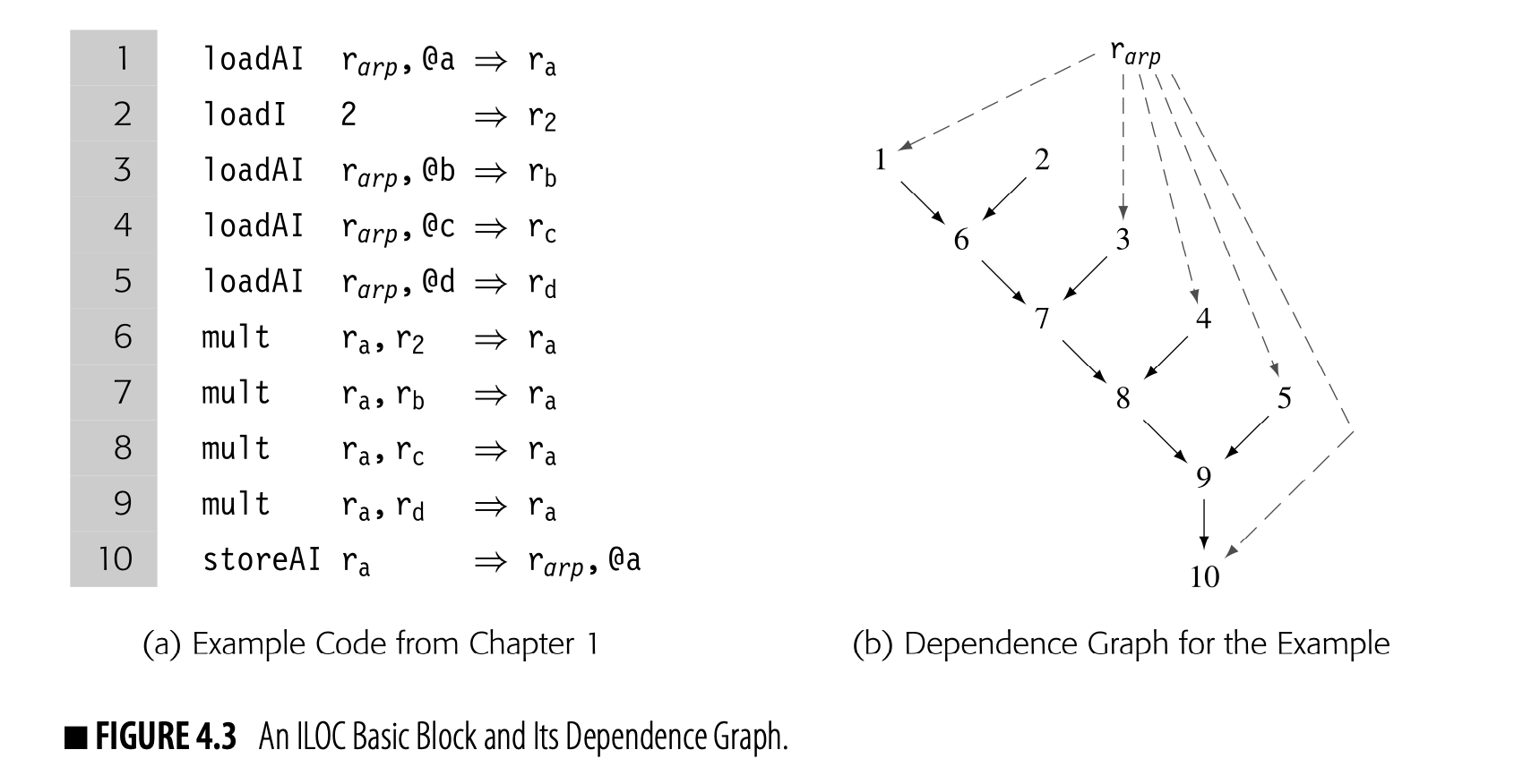
Fig. 4.3 shows ILOC code to compute a $a \leftarrow a \times 2 \times b \times c \times d$ , also shown in Fig. 4.4. Panel (a) contains the ILOC code. Panel (b) shows the corresponding data-dependence graph.

The dependence graph has a node for each operation in the block. Each edge shows the flow of a single value. For example, the edge from 3 to 7 reflects the definition of $r_{b}$ in statement 3 and its subsequent use in statement 7. The virtual register $r_{σ r p}$ contains an address that is at a fixed distance from the start of the local data area. Uses of $r_{σ r p}$ refer to its implicit definition at the start of the procedure; they are shown with dashed lines.

The edges in the graph represent real constraints on the sequencing of operations--a value cannot be used until it has been defined. The dependence graph edges impose a partial order on execution. For example, the graph requires that 1 and 2 precede 6. Nothing, however, requires that 1 or 2 precedes 3. Many execution sequences preserve the dependences shown in the graph, including $(1, 2, 3, 4, 5, 6, 7, 8, 9, 10)$ and $(2, 1, 6, 3, 7, 4, 8, 5, 9, 10)$ . The instruction scheduler exploits the freedom in this partial order, as does an "out-of-order" processor.

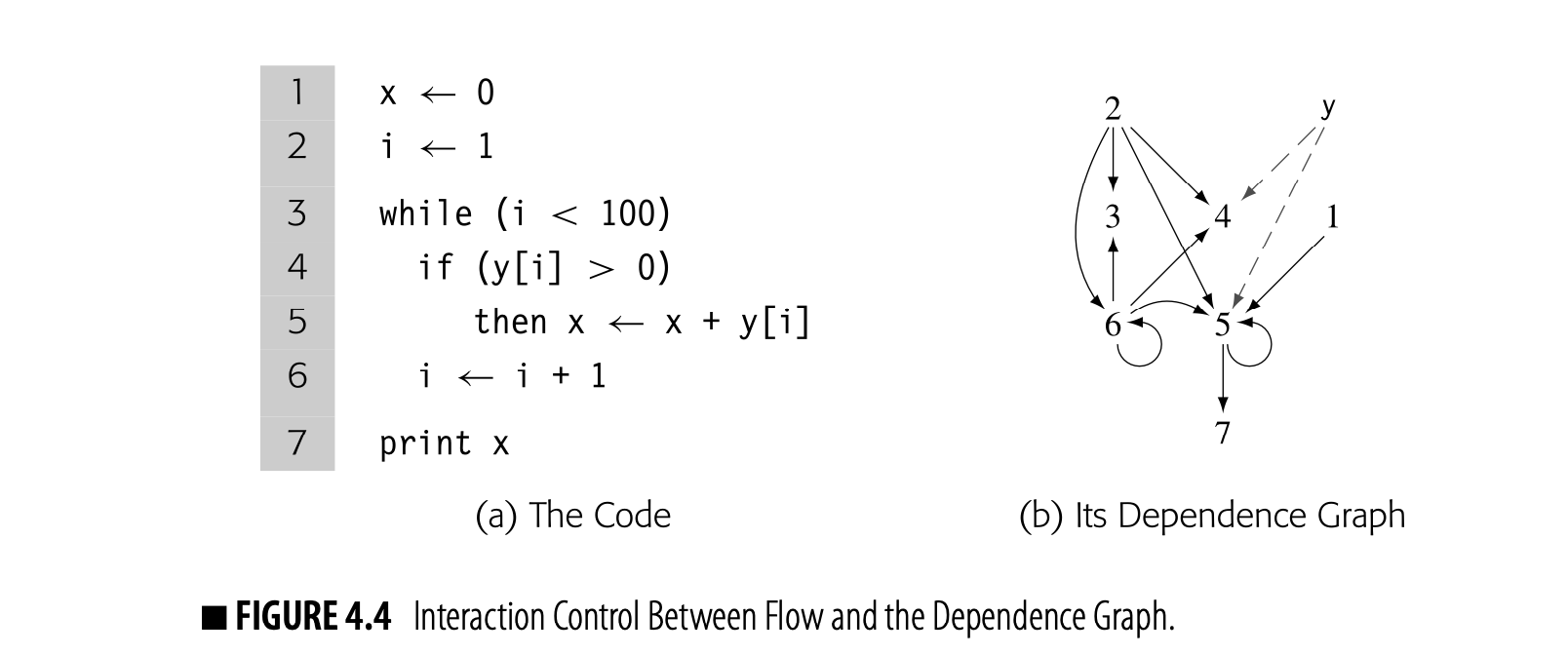
At a more abstract level, consider the code fragment shown in Fig. 4.4(a), which incorporates multiple basic blocks, along with both a while loop and an if-then construct. The compiler can construct a single dependence graph for the entire code fragment, as shown in panel (b).

References to $y [i]$ derive their values from a single node that represents all of the prior definitions of $y$ . Without sophisticated analysis of the subscript expressions, the compiler cannot differentiate between references to individual array elements.

This dependence graph is more complex than the previous example. Nodes 5 and 6 both depend on themselves; they use values that they may have defined in a previous iteration. Node 6, for example, can take the value of $i$ from either 2 (in the initial iteration) or from itself (in any subsequent iteration). Nodes 4 and 5 also have two distinct sources for the value of $i$ : nodes 2 and 6.

Mode of Use: Data-dependence graphs are typically built for a specific task and then discarded, making them a derivative IR. They play a central role in instruction scheduling (Chapter 12). They find application in a variety of optimizations, particularly transformations that reorder loops to expose parallelism and to improve memory behavior. In more sophisticated applications of the data-dependence graph, the compiler may perform ex- tensive analysis of array subscript values to determine when references to the same array can overlap.

Call Graph

Interprocedural Any technique that examines interactions across more than one procedure is called interprocedural.

To optimize code across procedure boundaries, some compilers perform interprocedural analysis and optimization. To represent calls between procedures, compilers build a call graph. A call graph has a node for each procedure and an edge for each distinct procedure call site. Thus, if the code calls $q$ from three textually distinct sites in $p$ , the call graph has three edges $(p, q)$ , one for each call site.

Intraprocedural Any technique that limits its attention to a single procedure is called intraprocedural.

Both software-engineering practice and language features complicate the construction of a call graph.

Call graph a graph that represents the calling relation- ships among the procedures in a program The call graph has a node for each proce- dure and an edge for each call site.

Separate compilation limits the compiler's ability to build a call graph because it limits the set of procedures that the compiler can see. Some compilers build partial call graphs for the procedures in a compilation unit and optimize that subset.
Procedure-valued parameters, both as actual parameters and as return values, create ambiguous calls that complicate call-graph construction. The compiler may perform an interprocedural analysis to limit the set of edges that such a call induces in the call graph, making call graph construction a process of iterative refinement. (This problem is analogous to the issue of ambiguous branches in CFG construction, as discussed in Section 4.4.4.)

Class hierarchy analysis a static analysis that builds a model of a program’s inheritance hierarchy

In object-oriented programs, inheritance can create ambiguous procedure calls that can only be resolved with additional type information. In some languages, class hierarchy analysis can disambiguate many of these calls; in others, that information cannot be known until runtime. Runtime resolution of ambiguous calls poses a serious problem for call graph construction; it also adds significant runtime overhead to the ambiguous calls.

Section 9.4 discusses some of the problems in call graph construction.

Mode of Use: Call graphs almost always appear as a derivative IR, built to support interprocedural analysis and optimization and then discarded. In fact, the best known interprocedural transformation, inline substitution (see Section 8.7.1), changes the call graph as it proceeds, rendering the old call graph inaccurate.

SECTION REVIEW

Graphical IRs present an abstract view of the code being compiled. The level of abstraction in a graphical IR, such as an AST, can vary from source level to below machine level. Graphical IRs can serve as definitive IRs or be built as special-purpose derivative IRs.

Because they are graphs, these IRs encode relationships that may be difficult to represent or manipulate in a linear IR. Graph traversals are an efficient way to move between logically connected points in the program; most linear IRs lack this kind of cross-operation connectivity.

REVIEW QUESTIONS

Given an input program, compare the expected size of the IR as a func- tion of the number of tokens returned by the scanner for (a) a parse tree, (b) an AST, and (c) a DAG. Assume that the nodes in all three IR forms are of a uniform and fixed size.

How does the number of edges in a dependence graph for a basic block grow as a function of the number of operations in the block?

4.4 Linear IRs

Linear IRs represent the program as an ordered series of operations. They are an alternative to the graphical IRs described in the previous section. An assembly-language program is a form of linear code. It consists of an ordered sequence of instructions. An instruction may contain more than one operation; if so, those operations execute in parallel. The linear IRs used in compilers often resemble the assembly code for an abstract machine.

The logic behind using a linear form is simple. The source code that serves as input to the compiler is a linear form, as is the target-machine code that it emits. Several early compilers used linear IRs; this was a natural notation for their authors, since they had previously programmed in assembly code.

Linear IRs impose a total order on the sequence of operations. In Fig. 4.3, contrast the ILOC code with the data-dependence graph. The ILOC code has an implicit total order; the dependence graph imposes a partial order that allows multiple execution orders.

If a linear IR is used as the definitive IR in a compiler, it must include a mechanism to encode transfers of control among points in the program. Control flow in a linear IR usually models the implementation of control flow on the target machine. Thus, linear codes usually include both jumps and conditional branches. Control flow demarcates the basic blocks in a linear IR; blocks end at branches, at jumps, or just before labeled operations.

Taken branch In most ISAs, conditional branches use only one label. Control flows either to the label, called the taken branch, or to the operation that follows the label, called the fall-through branch. The fall-through path is often faster than the taken path.

Branches in I L O C differ from those found in a typical assembly language. They explicitly specify a label for both the taken path and the fall-through path. This feature eliminates all fall-through transfers of control and makes it easier to find basic blocks, to reorder basic blocks, and to build a CFG.

Many kinds of linear IRs have been used in compilers.

■ One-address codes model the behavior of accumulator machines and stack machines. These codes expose the machine’s use of implicit names so that the compiler can tailor the code for it. The resulting IR can be quite compact.

Destructive operation an operation in which one of the operands is always redefined with the result These operations likely arose as a way to save space in the instruction format on 8- or 16-bit machines.

■ Two-address codes model a machine that has destructive operations. These codes fell into disuse as destructive operations and memory con- straints on IR size became less important; a three-address code can model destructive operations explicitly.

■ Three-address codes model a machine where most operations take two operands and produce a result. The rise of RISC architectures in the 1980s and 1990s made these codes popular again.

The rest of this section describes two linear IRs that are in common use: stack-machine code and three-address code. Stack-machine code offers a compact, storage-efficient representation. In applications where IR size mat- ters, such as a JAVA applet transmitted over a network before execution, stack-machine code makes sense. Three-address code models the instruction format of a modern RISC machine; it has distinct names for two operands and a result. You are already familiar with one three-address code: the ILOC used throughout this book.

4.4.1 Stack-Machine Code

Stack-machine code, a form of one-address code, assumes the presence of a stack of operands. It is easy to generate and to understand. Most operations read their operands from the stack and push their results onto the stack. For example, a subtract operator removes the top two stack elements and pushes their difference onto the stack.

The stack discipline creates a need for new operations: push copies a value from memory onto the stack, pop removes the top element of the stack and writes it to memory, and swap exchanges the top two stack elements. Stack-based processors have been built; the IR seems to have appeared as a modelfor those ISAs. Stack-machine code for the expression a - 2xb appears in the margin. Stack-machine code is compact. The stack creates an implicit name space and eliminates many names from the IR, which shrinks the IR. Using the stack, however, means that all results and arguments are transitory, unless the code explicitly moves them to memory.

Bytecode an IR designed specifically for its compact form; typically code for an abstract stack machine The name derives from its limited size; many operations, such as multiply, need only a single byte.

Mode of Use: Stack-machine code is typically used as a definitive ir--often as the IR to transmit code between systems and environments. Both SMALLtalk-80 and JAVA use bytecode, the ISA of a stack-based virtual machine, as the external, interpretable form for code. The bytecode either runs in an interpreter, such as the JAVA virtual machine, or is translated into native target-machine code before execution. This design creates a system with a compact form of the program for distribution and a simple scheme for porting the language to a new machine: implement an interpreter for the virtual machine.

4.4.2 Three-Address Code

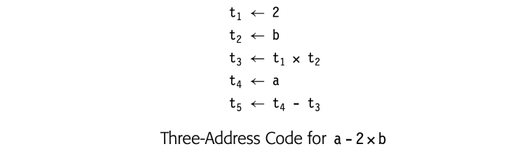In three-address code, most operations have the form i - j op k, with an operator (op), two operands (j and k), and one result (i). Some operators, such as an immediate load and a jump, use fewer arguments. Sometimes, an operation has more than three addresses, such as a floating-point multiply-add operation. Three-address code for a - 2xb appears in the margin. ILOC is a three-address code.

Three-address code is attractive for several reasons. First, it is reasonably compact. Most operations consist of four items: an operation code, or opcode, and three names. The opcode and the names are drawn from limited sets. Opcodes typically require one or two bytes. Names are typically represented by integers or table indices. Second, separate names for the operands and the result give the compiler freedom to specify and control the reuse of names and values; three-address code has no destructive operations. Three-address code introduces a new set of compiler-generated names--names that hold the results of the various operations. A carefully chosen name space can reveal new opportunities to improve the code. Finally, since many modern processors implement three-address operations, a three-address code models their properties well.

Level of Abstraction: Within three-address codes, the set of supported operators and the level of abstraction can vary widely. Often, a three-address IR will contain mostly low-level operations, such as jumps, branches, loads, and stores, alongside more complex operations that encapsulate control flow, such as max. Representing these complex operations directly simplifies analysis and optimization.

For example, consider an operation that copies a string of characters from one address, the source, to another, the destination. This operation appeared as the bcopy library routine in the 4.2 BSD UNIX distribution and as the mvcl instruction (move character long) in the IBM 370 ISA. On a machine that does not implement an operation similar to mvcl, it may take many operations to perform such a copy.

IBM’s PL.8 compiler, a pioneering RISC compiler, used this strategy.

Adding mvcl to the three-address code lets the compiler compactly represent this complex operation. The compiler can analyze, optimize, and move the operation without concern for its internal workings. If the hardware supports an mvcl-like operation, then code generation will map the IR construct directly to the hardware operation. If the hardware does not, then the compiler can translate mvcl into a sequence of lower-level IR operations or a call to a bcopy-like routine before final optimization and code generation.

Mode of Use: Compilers that use three-address codes typically deploy them as a definitive IR. Three-address code, with its explicit name space and its load-store memory model, is particularly well suited to optimization for register-to-register, load-store machines.

4.4.3 Representing Linear Codes

Many data structures have been used to implement linear IRs. The choices that a compiler writer makes affect the costs of various operations on IR code. Since a compiler spends most of its time manipulating the IR form of the code, these costs deserve some attention. While this discussion focuses on three-address codes, most of the points apply equally to stack-machine code (or any other linear form).

Three-address codes are often implemented as a set of quadruples. Each quadruple is represented with four fields: an operator, two operands (or sources), and a destination. To form blocks, the compiler needs a mechanism to connect individual quadruples. Compilers implement quadruples in a variety of ways.

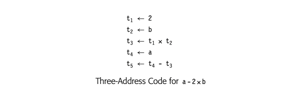Fig. 4.5 shows three schemes to represent three-address code for a-2xb (shown in the margin). The first scheme, in panel (a), uses an array of structures. The compiler might build such an array for each CFG node to hold the code for the corresponding block. In panel (b), a vector of pointers holds the block's quadruples. Panel (c) links the quadruples together into a list.

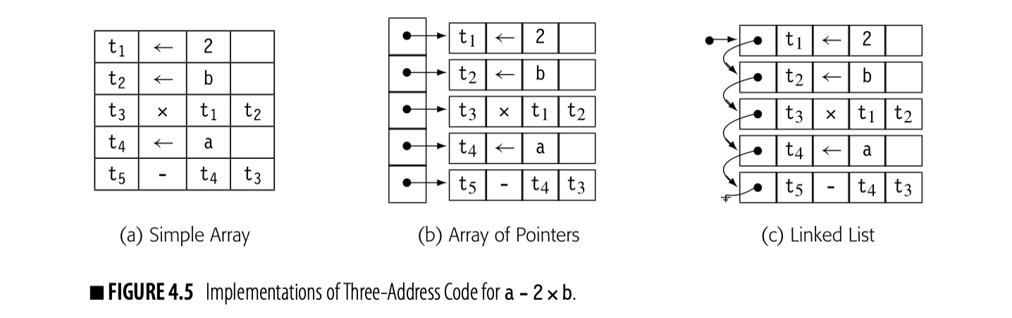
Consider the costs incurred to rearrange the code in this block. The first operation loads a constant into a register; on most machines this translatesdirectly into a load immediate operation. The second and fourth operations load values from memory, which on most machines might incur a multicycle delay unless the values are already in the primary cache. To hide some of the delay, the instruction scheduler might move the loads of b and a in front of the load immediate of 2.

In the array of structures, moving the load of b ahead of the immediate load requires saving the first operation to a temporary location, shuffling the second operation upward, and moving the immediate load into the second slot. The vector of pointers requires the same three-step approach, except that only the pointer values must be changed. The compiler can save the pointer to the immediate load, copy the pointer to the load of b into the first vector element, and rewrite the second vector element with the saved pointer. For the linked list, the operations are similar, except that the compiler must save enough state to let it traverse the list.

Now, consider what happens in the front end when it generates the initial round of ir. With the array of structures and the vector of pointers, the compiler must select a size for the array--in effect, the number of quadruples that it expects in a block. As it generates the quadruples, it fills in the data structure. If the compiler allocated too much space, that space is wasted. If it allocated too little, the compiler must allocate space for a larger array or vector, copy the contents into this new place, and free the original space. The linked list avoids these problems. Expanding the list just requires allocating a new quadruple and setting the appropriate pointer in the list.

A multipass compiler may use different implementations to represent the ir at different points in the compilation process. In the front end, where the focus is on generating the ir, a linked list might both simplify the implementation and reduce the overall cost. In an instruction scheduler, with its focus on rearranging the operations, the array of pointers might make more sense. A common interface can hide the underlying implementation differences.

INTERMEDIATE REPRESENTATIONS IN ACTUAL USE

In practice, compilers use a variety of IRs. Legendary FORTRAN compilers of yore, such as IBM’s FORTRAN H compilers, used a combination of quadruples and control-flow graphs to represent the code for optimization. Since FORTRAN H was written in FORTRAN, it held the IR in an array.

For years, GCC relied on a very low-level IR, called register transfer language (RTL). GCC has since moved to a series of IRs. The parsers initially produce a language-specific, near-source tree. The compiler then lowers that tree to a second IR, GIMPLE, which includes a language-independent tree-like structure for control-flow constructs and three-address code for expressions and assignments. Much of GCC’s optimizer uses GIMPLE; for example, GCC builds static single-assignment form (SSA) on top of GIMPLE. Ultimately, GCC translates GIMPLE into RTL for final optimization and code generation.

The LLVM compiler uses a single low-level IR; in fact, the name LLVM stands for “low-level virtual machine.” LLVM’s IR is a linear three-address code. The IR is fully typed and has explicit support for array and structure addresses. It provides support for vector or SIMD data and operations. Scalar values are maintained in SSA form until the code reaches the compiler’s back end. In LLVM environments that use GCC front ends, LLVM IR is produced by a pass that performs GIMPLE-to-LLVM translation.

The Open64 compiler, an open-source compiler for the IA-64 architecture, used a family of five related IRs, called WHIRL. The parser produced a near-source-level WHIRL. Subsequent phases of the compiler introduced more detail to the WHIRL code, lowering the level of abstraction toward the actual machine code. This scheme let the compiler tailor the level of abstraction to the various optimizations that it applied to IR.

Notice that some information is missing from Fig. 4.5. For example, no labels are shown because labels are a property of the block rather than any individual quadruple. Storing a list of labels with the CFG node for the block saves space in each quadruple; it also makes explicit the property that labels occur only at the start of a block. With labels attached to a block, the compiler can ignore them when reordering operations inside the block, avoiding one more complication.

4.4.4 Building the CFG from Linear Code

Compilers often must convert between different its, often different styles of its. One routine conversion is to build a CFG from a linear IR such as ILOC. The essential features of a CFG are that it identifies the beginning and end of each basic block and connects the resulting blocks with edges thatdescribe the possible transfers of control among blocks. Often, the compiler must build a CFG from a simple, linear IR that represents a procedure.

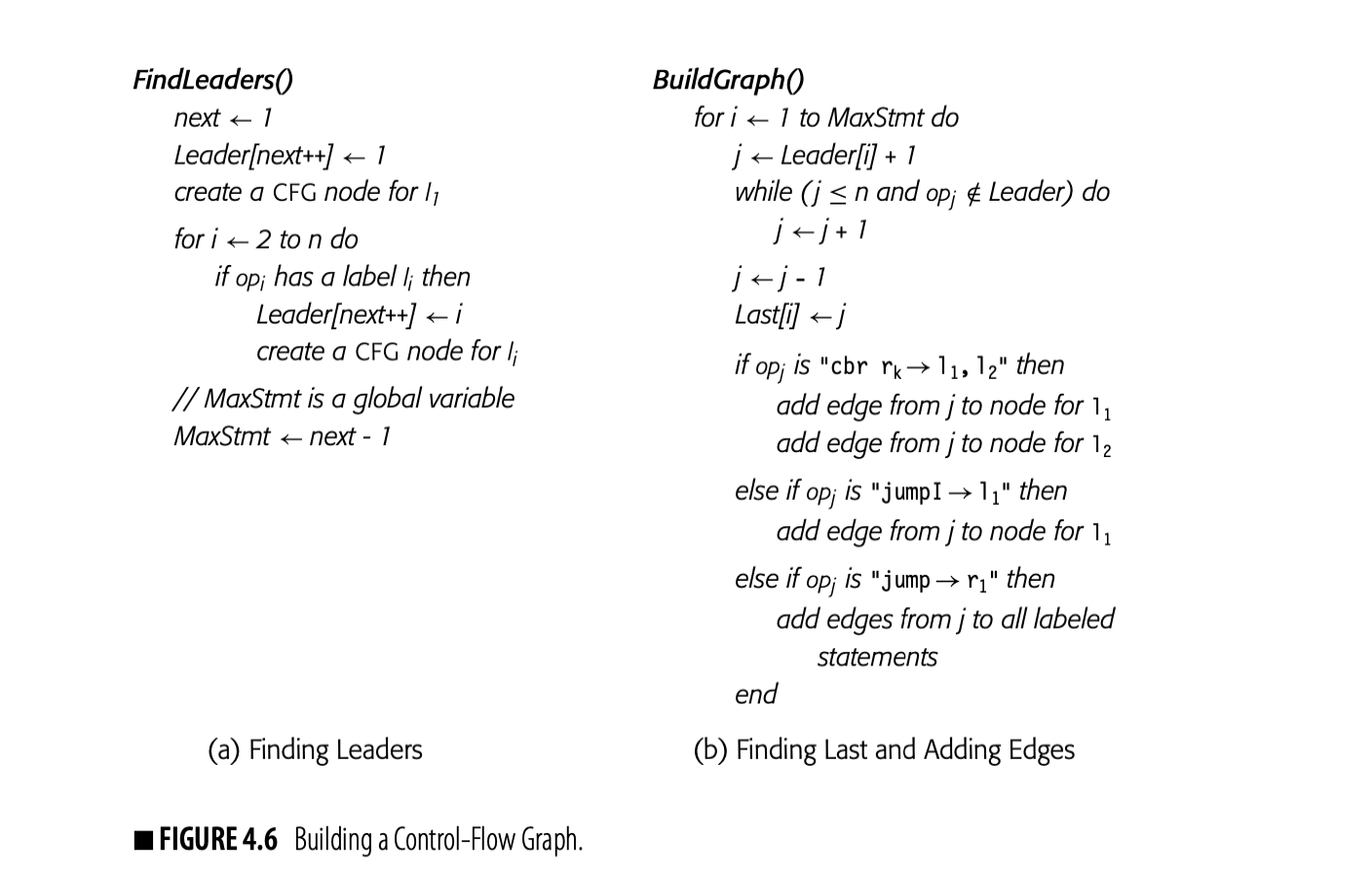
As a first step, the compiler must find the start and the end of each basic block in the linear IR. We will call the initial operation of a block a leader. An operation is a leader if it is the first operation in the procedure, or if it has a label that is, potentially, the target of some branch. The compiler can identify leaders in a single pass over the IR, shown in Fig. 4.6(a). FindLeaders iterates over the operations in the code, in order, finds the labeled statements, and records them as leaders.

Ambiguous jump a branch or jump whose target is not known at compile time (e.g., a jump to an address in a register) In ILOC, jump is ambiguous while jumpI is not.

If the linear IR contains labels that are not used as branch targets, then treating labels as leaders may unnecessarily split blocks. The algorithm could track which labels are jump targets. However, ambiguous jumps may force it to treat all labeled statements as leaders.

CFG construction with fall-through branches is left as an exercise for the reader (see Exercise 4).

The second pass, shown in panel (b), finds every block-ending operation. It assumes the ILOC model where every block, except the final block, ends with a branch or a jump and branches specify labels for both the taken and not-taken paths. This assumption simplifies the handling of blocks and allows the compiler's optimizer or back end to choose which path will be the "fall through" case of a branch. (For the moment, assume branches have no delay slots.)

To find the end of each block, the algorithm iterates through the blocks, in order of their appearance in the Leader array. It walks forward through the IR until it finds the leader of the next block. The operation immediately before that leader ends the current block. The algorithm records that operation's index in $L os t [j]$ , so that the pair \text{\langle Leader[j], Lost[j] \rangle} describes block $i$ . It adds edges to the CFG as needed.

For a variety of reasons, the CFG should have a unique entry node $n_{0}$ and a unique exit node $n_{f}$ . If the underlying code does not have this shape, a simple postpass over the graph can create $n_{0}$ and $n_{f}$ .

Complications in CFG Construction

Features of the IR, the target machine, and the source language can complicate CFG construction.

Pseudooperation an operation that manipulates the internal state of the assembler or compiler, but does not translate into an executable operation

Ambiguous jumps may force the compiler to add edges that are not feasible at runtime. The compiler writer can improve this situation by recording the potential targets of ambiguous jumps in the IR. IOC includes the tb1 pseudooperation to specify possible targets of an ambiguous jump (see Appendix A). Anytime the compiler generates a jump, it should follow the jump with one or more tb1 operations that record the possible targets. The hints reduce spurious edges during CFG construction.

PC-relative branch A transfer of control that specifies an offset, either positive or negative, from its own memory address.

If a tool builds a CFG from target-machine code, features of the target ISA can complicate the process. The algorithm in Fig. 6.4.6 assumes that all leaders, except the first, are labeled. If the target machine has fall-through branches, the algorithm must be extended to recognize unlabeled statements that receive control on a fall-through path. PC-relative branches cause a similar set of complications.

Branch delay slots introduce complications. The compiler must group any operation in a delay slot into the block that preceded the branch or jump. If that operation has a label, it is a member of multiple blocks. To disambiguate such an operation, the compiler can place an unlabeled copy of the operation in the delay slot and use the labeled operation to start the new block.

If a branch or jump can occur in a branch delay slot, the CFG builder must walk forward from the leader to find the block-ending branch--the first branch it encounters. Branches in the delay slot of a block-ending branch can be pending on entry to the target block. In effect, they can split the target block into multiple blocks and create both new blocks and new edges. This feature adds serious complications to CFG construction.

Some languages allow jumps to labels outside the current procedure. In the procedure that contains the jump, the jump target can be modeled with a new block. In the procedure that contains the target, however, the labeled block can pose a problem. The compiler must know that the label is the target of a nonlocal jump; otherwise, analysis passes may produce misleading results. For this reason, languages such as PASCAL or ALGOL restricted nonlocal jumps to visible labels in outer lexical scopes. C requires the use of the functions setjmp and longjmp to expose these transfers.

SECTION REVIEW

Linear IRs represent the code being compiled as an ordered sequence of operations. Linear IRs vary in their level of abstraction; the source code for a program in a text file is a linear form, as is the assembly code for that same program. Linear IRs lend themselves to compact, human-readable representations.

Two widely used linear IRs are bytecodes, generally implemented as a one-address code with implicit names on many operations, and three-address code, similar to ILOC.

REVIEW QUESTIONS

Consider the expression $a \times 2 + a \times 2 \times b$ . Translate it into stack-machine code and into three address code. Compare and contrast the total num- ber of operations and operands in each form. How do they compare to the tree in Fig. 4.2(b)?

Sketch the modifications that must be made to the algorithm in Fig. 4.6 to account for ambiguous jumps and branches. If all jumps and branches are labeled with a construct similar to ILOC’s tbl, does that simplify your algorithm?

4.5 Symbol Tables

Symbol table

A collection of one or more data structures that hold information about names and values Most compilers maintain symbol tables as persistent ancillary data structures used in conjunction with the IR that represents the executable code.

During parsing the compiler discovers the names and properties of many distinct entities, including named values, such as variables, arrays, records, structures, strings, and objects; class definitions; constants; labels in the code; and compiler-generated temporary values (see the digression on page 192).

For each name actually used in the program, the compiler needs a variety of information before it can generate code to manipulate that entity. The specific information will vary with the kind of entity. For a simple scalar variable the compiler might need a data type, size, and storage location. For

a function it might need the type and size of each parameter, the type and size of the return value, and the relocatable assembly-language label of the function’s entry point.

Thus, the compiler typically creates one or more repositories to store de- scriptive information, along with an efficient way to locate the information associated with a given name. Efficiency is critical because the compiler will consult these repositories many times.

The compiler typically keeps a set of tables, often referred to as symbol tables. Conceptually, a symbol table has two principal components: a map from textual name to an index in a repository and a repository where that index leads to the name’s properties. An abstract view of such a table is shown in the margin.

Constant pool a statically initialized data area set aside for constant values

A compiler may use multiple tables to represent different kinds of informa- tion about different kinds of values. For names, it will need a symbol table that maps each name to its properties, declared or implicit. For aggregates, such as records, arrays, and objects, the compiler will need a structure table that records the entity’s layout: its constituent members or fields, their prop- erties, and their relative location within the structure. For literal constants, such as numbers, characters, and strings, the compiler will need to lay out a data area to hold these values, often called a constant pool. It will need a map from each literal constant to both its type and its offset in the pool.

4.5.1 Name Resolution

The primary purpose of a symbol table is to resolve names. If the compiler finds a reference to name $n$ at some point $p$ in a program, it needs a mechanism that maps $n$ back to its declaration in the naming environment that holds at $p$ . The map from name to declaration and properties must be well defined; otherwise, a program might have multiple meanings. Thus, programming languages introduce rules that specify where a given declaration of a name is both valid and visible.

Scope the region of a program where a given name can be accessed

In general, a scope is a contiguous set of statements in which a name is declared, visible, and accessible. The limits of a scope are marked by specific symbols in the language. Typically, a new procedure defines a new scope that covers its entire definition. C and C++ demarcate blocks with curly braces. Each block defines a new scope.

REPRESENTING REFERENCES IN THE IR

In the implementation of an IR, the compiler writer must decide how to represent a reference to a source language name. The compiler could simply record the lexeme; that decision, however, will require a symbol-table lookup each time that the compiler uses the reference.

The best alternative may be to store a handle to the relevant symbol table reference. That handle could be an absolute pointer to the table entry; it might be a pointer to the table and an offset within the table. Such a handle will allow direct access to the symbol table information; it should also enable inexpensive equality tests.

In most languages, scopes can nest. A declaration for $x$ in an inner scope obscures any definitions of $x$ in surrounding scopes. Nesting creates a hierarchy of name spaces. These hierarchies play a critical role in softwareengineering; they allow the programmer to choose local names without concern for their use elsewhere in the program.

The two most common name-space hierarchies are created by lexical scope rules and inheritance rules. The compiler must build tables to model each of these hierarchies.

Lexical Scopes

A lexical-scoping environment uses properly nested regions of code as scopes. A name $n$ declared in scope $s$ is visible inside $s$ . It is visible inside any scope nested in $s$ , with the caveat that a new declaration of $n$ obscures any declaration of $n$ from an outer scope.

Global scope an outer scope for names visible in the entire program

At a point $p$ in the code, a reference to $n$ maps to the first declaration of $n$ found by traversing the scopes from the scope containing the reference all the way out to the global scope. Lexically scoped languages differ greatly in the depth of nesting that they allow and the set of scopes that they provide. (Sections 5.4.1, 6.3.1, and 6.4.3 discuss lexical scopes in greater depth.)

Inheritance Hierarchies

Superclass and Subclass In a language with inheritance, if class x inherits members and properties from class y, we say that x is a subclass of y and y is the superclass of x. The terminology used to specify inheri- tance varies across languages. In JAVA, a subclass extends its superclass. In C++, a subclass is derived from its superclass.

Object-oriented languages (OOLs) introduce another set of scopes: the inheritance hierarchy. OOLs create a data-centric naming scheme for objects; objects have data and code members that are accessed relative to the object rather than relative to the current procedure.

In an OOL, explicitly declared subclass and superclass relationships define the inheritance hierarchy--a naming regime similar to the lexical hierarchy and orthogonal to it. Conceptually, subclasses nest within superclasses, just as inner scopes nest within outer scopes in a lexical hierarchy. The compiler builds tables to model subclass and superclass relationships, as well.

Hierarchical Tables

The compiler can link together tables, built for individual scopes, to represent the naming hierarchies in any specific input program. A typical program in an Algol-like language (all) might have a single linked set of tables to represent the lexically nested scopes. In an OOL, that lexical hierarchy would be accompanied by another linked set of tables to represent the inheritance hierarchy.

When the compiler encounters a reference in the code, it first decides whether the name refers to a variable (either global or local to some method) or an object member. That determination is usually a matter of syntax; languages differentiate between variable references and object references. For a variable reference, it begins in the table for the current scope and searches upward until it finds the reference. For an object member, it determines the object's class and begins a search through the inheritance hierarchy.

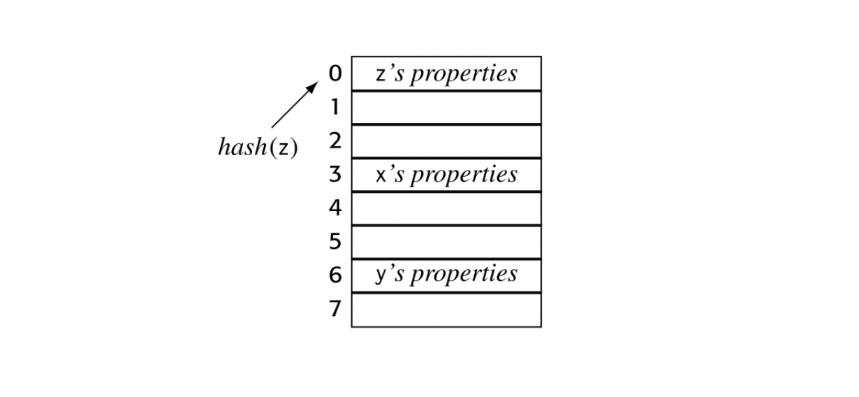
In a method $m$ , declared in some class $c$ , the search environment might look as follows. We refer to this scheme as the "sheaf of tables."

The lookup begins in the table for the appropriate scope and works its way up the chain of tables until it either finds the name or exhausts the chain. Chaining tables together in this fashion creates a flexible and powerful tool to model the complex scoping environments of a modern programming language.

The compiler writer can model complex scope hierarchies--both lexical hierarchies and inheritance hierarchies--with multiple tables linked together in a way that reflects the language-designated search order. For example, nested classes in JAVA give rise to a lexical hierarchy within the inheritance hierarchy. The link order may vary between languages, but the underlying technology need not change.

In a modern environment, the compiler will likely retain each of these tables for later use, either in the compiler or in related tools such as performance monitors or debuggers. The sheaf-of-tables approach can create compact, separable tables suitable for preservation.

Other Scopes

Other language features create nested scopes. For example, records, structures, and objects all act as independent scopes. Each creates a new name space and has a set of visibility rules. The compiler may or may not choose to implement these scopes with a full-blown sheaf in a hash table; nonetheless each is a distinct scope and can be modeled with a new sheaf in the appropriate table. The constant pool might also be treated as a separate scope.

4.5.2 Table Implementation

As we have seen, a compiler will contain multiple distinct tables, ranging from symbol tables and inheritance tables through structure layout tables and constant tables. For each table, the compiler writer must choose an appropriate implementation strategy: both a mapping function and a repository. While the choices are, for the most part, independent, the compiler writer may want to use the same basic strategies across multiple tables so that they can share implementations.

Implementing the Mapping

The mapping from a textual name to an index can be implemented in myriad ways, each with their own advantages and disadvantages.

Linear List

A linear list is simple to construct, to expand, and to search. The primary disadvantage of a linear list is that searching the list takes \mathsf{O}\big{(}n\big{)} time per lookup, where $n$ is the number of items in the list. Still, for a small procedure, a linear list might make sense.

Tree

A tree structure has the advantages of a list, including simple and efficient expansion. It also has the potential to significantly reduce the time required per lookup. Assuming that the tree is roughly balanced--that is, the subtrees at each level are approximately the same size--then the expected case lookup time should approach \mathsf{O}\big{(}\log_{2}n\big{)} per item, where $n$ is the number of items in the tree.

Balanced trees use more complex insertion and deletion protocols to maintain roughly equal-sized subtrees. The literature contains many effective and efficient techniques for building balanced trees.

Unbalanced trees have simpler insertion and deletion protocols but provide no guarantees on the relative sizes of sibling subtrees. An unbalanced tree can devolve into linear search when presented with an adversarial input.

Hash Map

The compiler can use a numerical computation, called a hash, to produce an integer from a string. A well-designed hash function,, distributes those integers so that few strings produce the same hash value. To build a hash table, the programmer uses the hash value of a string, modulo the table size, as an index into a table.

Hash collision When two strings map to the same table index, we say that they collide. For hash function h(x) and table size s, if $h (x) mod s = h (y) mod s,$ then x and y will collide.

Handling collisions is a key issue in hash table design, as discussed in Appendix B.4. If the set of keys produces no collisions, then insertion and lookup in a hash table should take $O (1)$ . If the set of keys all map to the same table index, then insertion and lookup might devolve to $O (∣ k eys ∣)$ time per lookup. To avoid this problem, the compiler writer should use a well-designed hash function, as found in a good algorithms textbook.

Static Map

As an alternative to hashing, the compiler can precompute a collision-free static map from keys to indices. Multiset discrimination solves this problem (see the digression on page 190).

For small sets of keys, an approach that treats the keys as a set of acyclic regular expressions and incrementally builds a to recognize that set can lead to a fast implementation (see Section 2.6.2). Once the transition-table size exceeds the size of the level-one data cache, this approach slows down considerably.

Implementing the Repository

The implementation of the repository storage for the information associated with a given name can be orthogonal to the lookup mechanism. Different tables may need distinct and different structures to accommodate the kinds of information that the compiler needs. Nonetheless, these repositories should have some common properties (see also Appendix B.4).

Block contiguous These allocators use two protocols: a ma- jor allocation obtains space for multiple records while a minor one returns a single record. Minor allocations use a fast method; they amortize the major allocation cost over many records.

Record storage should be either contiguous or block-contiguous to improve locality, decrease allocation costs, and simplify reading and writing the tables to external media.
Each repository should contain enough information to rebuild the lookup structure, in order to accommodate graceful table expansion, and to facilitate restoring the structures from external media.
The repository should support changes to the search path. For example, as the parser moves in and out of different scopes, the search path should change to reflect the current situation.

From a management perspective, the repository must be expandable in order to handle large programs efficiently without wasting space on small ones. Its index scheme should be independent of the mapping scheme so that the map can be expanded independently of the repository; ideally, the map will be sparse and the repository dense.

SECTION REVIEW

Compilers build ancillary data structures to augment the information stored in the compiler’s definitive IR. The most visible of these structures is a set of symbol tables that map a name in the source text or the IR into the set of properties associated with that name.

This section explored several issues in the design of these ancillary tables. It showed how linking tables together in explicit search paths can model both lexical scope rules and inheritance rules. It discussed tradeoffs in the implementation of both the mapping mechanism and the repository for these tables.

REVIEW QUESTIONS

Using the “sheaf-of-tables” scheme, what is the complexity of inserting a new name into the table at the current scope? What is the complexity of looking up a name in the set of tables? How deep are the lexical and inheritance hierarchies in programs that you write?

When the compiler initializes a scope, it likely needs an initial symbol table size. How might the parser estimate that initial symbol table size? How might later passes of the compiler estimate it?

4.6 Name Spaces

Most discussions of name spaces focus on the source program's name space: lexical scopes and inheritance rules. Of equal importance, from the perspective of the quality of compiled code, is the name space created in the compiler's IR. A specific naming discipline can either expose opportunities for optimization or obscure them. The choices that the compiler makes with regard to names determine, to a large extent, which computations can be analyzed and optimized.

AN ALTERNATIVE TO HASHING

Symbol tables are often implemented with hash maps, due to the expected efficiency of hashing. If the compiler writer is worried about the unlikely but possible worst-case behavior of hashing, multiset discrimination provides an interesting alternative. It avoids the possibility of worst-case behavior by constructing the index offline, in the scanner.

To use multiset discrimination, the compiler first scans the entire program and builds a ⟨name,pos⟩ tuple for each instance of an identifier, where name is the identifier’s lexeme and pos is its ordinal position in the list of classified words, or tokens. It enters all the tuples into a large set.

Next, the compiler sorts the set lexicographically. In effect, this creates a set of subsets, one per identifier. Each subset holds the tuples for all the occurrences of its identifier. Since each tuple refers to a specific token, through its position value, the compiler can use the sorted set to modify the token stream. The compiler makes a linear scan over the set, processing each subset. It allocates a symbol-table index for each unique identifier, then rewrites the tokens to include that index. The parser can read symbol-table indices directly from the tokens. If the compiler needs a textual lookup function, the resulting table is ordered alphabetically for a binary search.

This technique adds some cost to compilation. It makes an extra pass over the token stream, along with a lexicographic sort. In return, it avoids any possibility of worst-case behavior from hashing and it makes the initial size of the symbol table obvious before parsing begins. This technique can replace a hash table in almost any application in which an offline solution will work.

The IR name space is intimately related to the memory model used in translation. The compiler may assume that all values are kept in memory, except when they are actively used in a computation. The compiler may assume that values are kept in registers whenever possible. If the compiler uses stack-machine code as its IR, it will keep these active values on the stack. These different assumptions radically affect the set of values that can be named, analyzed, and optimized.

This section focuses on issues in name space design; it also introduces one important example: static single assignment form. The next section explores the issues that arise in choosing a memory model.

4.6.1 Name Spaces in the IR

When compiler writers design an IR, they should also design a naming discipline for the compiler to follow. The choice of a name space interacts with the choice of an IR; some IRs allow broad latitude in naming, while others make most names implicit in the representation.

Implicit Versus Explicit Names

Tree-like IRs use implicit names for some values. Consider an AST for $a - 2 \times b$ , shown in the margin. It has nodes for each of a, 2, b, $2 \times b$ , and $a - 2 \times b$ . The interior nodes, those for $2 \times b$ and $a - 2 \times b$ , lack explicit names that the compiler can manipulate. 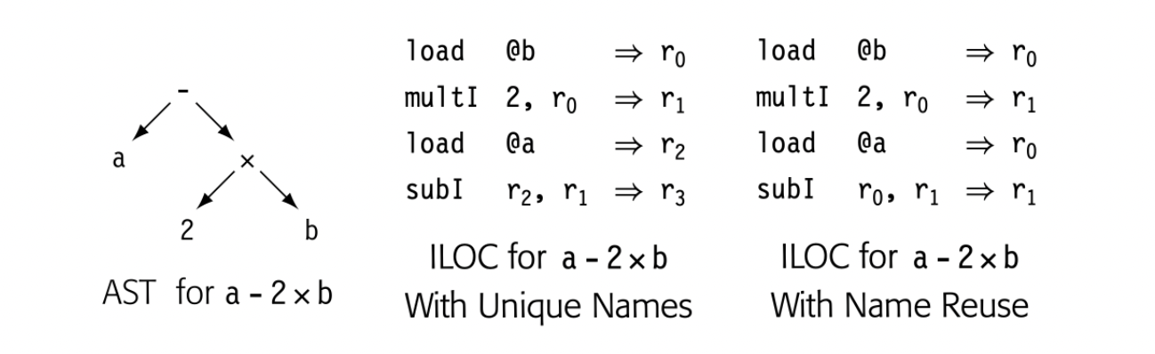By contrast, three-address code uses only explicit names, which gives the compiler control over the naming discipline. It can assign explicit names to any or all of the values computed in the code. Consider, for example, the ILOC code for a-2xb, shown in the margin. The upper version introduces a unique name for every unknown value and expression--register names $r_{0}$ through $r_{3}$ . After execution, each of those values survives in its own register. The lower version uses a different naming discipline intended to conserve names. After it executes, the two quantities that survive are a in $r_{0}$ and a-2xb in $r_{1}$ .

The example makes it appear that graphical IRs use implicit names and linear IRs use explicit names. It is not that simple. Stack-machine code relies on an implicit stack data structure, which leads to implicit names for many values. A CFG has explicit names for each of the nodes so that they can be connected to the corresponding code fragments. Even an AST can be rewritten to include explicit names; for any expression or subexpression that the compiler wants to name, it can insert an assignment and subsequent use for a compiler-generated name.

Variables Versus Values

In the source program, the set of accessible names is determined by the source language rules and the details of the program. Declared named variables are visible; intermediate subexpressions are not. In the statement: a, b, and c can each be used in subsequent statements. The values of 2*b, c/3, and cos(c/3) cannot.

Virtual name A compiler-generated name is often called a virtual name, in the same sense as virtual memory or a virtual register.

In the IR form of the code, the compiler writer must decide which values to expose via consistent, explicit names. The compiler can use as many names as necessary; compiler writers sometimes refer to these generated names as virtual names. The compiler might translate the statement so that the code evaluates each of these three expressions into its own unique name. Alternatively, by reusing names, it could eliminate any chance for reuse.

The impact of naming

In the late 1980s, we experimented with naming schemes in a FORTRAN 77 compiler. The first version generated a new name for each computation; it simply bumped a counter to get a new name. This approach produced large name spaces; for example, 985 names for a 210-line implementation of the singular value decomposition (SVD). Objectively, this name space seemed large. It caused speed and space problems in the register allocator, where name space size determines the size of many data structures. (Today, we have better data structures, and much faster machines with more memory).

The second version used an allocate/free protocol to manage names. The front end allocated temporary names on demand and freed them when the immediate uses were finished. This scheme shrank the name space; SVD used roughly 60 names. Allocation was faster; for example, the time to compute LwCount sets for SVD decreased by 60 percent (see Section 8.6.1).

Unfortunately, reuse of names obscured the flow of values and degraded the quality of optimization. The decline in code quality overshadowed any compile-time benefits.

Further experimentation led to a short set of rules that yielded strong optimization while mitigating growth in the name space.

Each textual expression received a unique name, found by hashing. Thus, each occurrence of an expression, for example, $r_{1} + r_{2L}$ targeted the same register.

In (op) $r_{i}, r_{j} \Rightarrow r_{k} k$ was chosen so that $i, j < k$ .

Register copy operations, $r_{i} \Rightarrow r_{j}$ , were allowed to have $i > j$ only if $r_{j}$ corresponded to a declared scalar variable. Registers for variables were only defined by copy operations. Expressions were evaluated into their "natural" register and then were moved into the register for the variable.

Each store operation, $r_{i} \Rightarrow MEM (r_{j})$ , was followed by a copy from $r_{i}$ into the variable's named register. (Rule 1 ensures that loads from that location always target the same register. Rule 4 ensures that the virtual register and memory location contain the same value.)

With this name space, the compiler used about 90 names for SVD. It exposed all of the optimizations found with the first name-space scheme. The compiler used these rules until we adopted the SSA name space.

This decision has a direct effect on what the compiler can do in subsequent optimization.

The compiler writer enforces these decisions by codifying them in the translation rules that generate the ir. These decisions have a widespread effect on the efficiency of both the compiler and the code that it generates.

The temptation, of course, is to provide a unique name for each subexpression, so as to maximize the opportunities presented to the optimizer. However, not all subexpressions are of interest. A value that is only live in a single block does not need a name that persists through the entire procedure. Exposing such a value to procedure-wide analysis and optimization is unlikely to change the code.

The converse is true, as well. Any value that is live in multiple blocks or is computed in multiple blocks may merit an explicit, persistent name. Expressions that are computed in multiple blocks, on multiple paths, are prime targets for a number of classical global optimizations. Providing a single consistent name across multiple definitions and uses can expose an expression to analysis and transformations that improve the compiled code (see Chapters 8-10).

Finally, the choice of a naming discipline also interacts with decisions about the level of abstraction in the IR. Consider again the two representations of an array reference, a[i,j], shown in the margin. The source-level AST, along with the symbol table, contains all of the essential information needed to analyze or translate the reference. (The symbol table will contain a's type, data area, and offset in that data area along with the number of dimensions and their upper and lower bounds.) The corresponding ILOC code exposes more details of the address calculations and provides explicit names for each subexpression in that calculation.

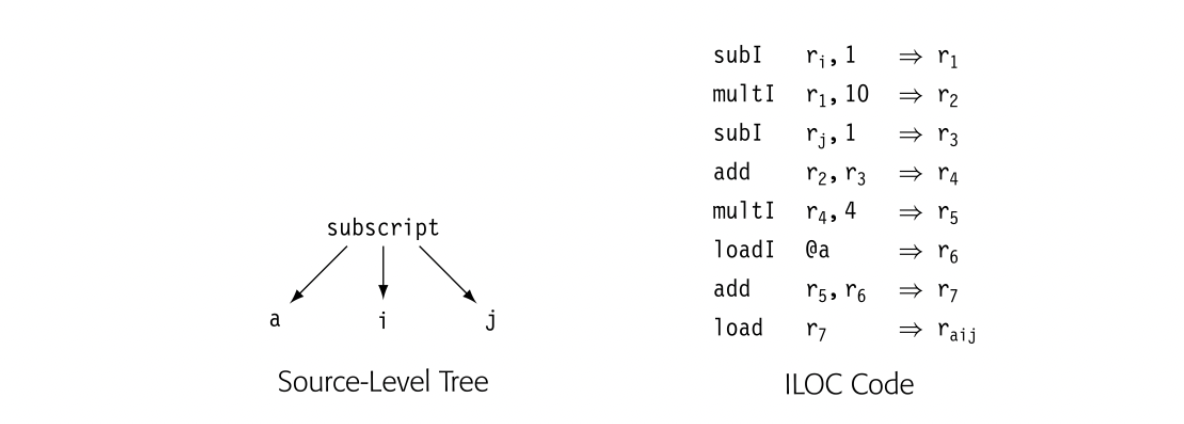
These two representations expose and name different quantities. The AST explicitly exposes the fact that the calculation computes the address for a[i,j], but shows no details of that calculation. The ILOC code exposes the fact that the address computation involves seven distinct subexpressions, any one of which might occur elsewhere. The question of which IR is better depends entirely on how the compiler writer intends to use the information.

4.6.2 Static Single-Assignment Form

SSA form an IR that has a value-based name system, created by renaming and use of pseudoop- erations called $ϕ$ -functions SSA encodes both control and value flow. It is used widely in optimization (see Section 9.3).

Static single-assignment form (SSA) is an IR and a naming discipline that many modern compilers use to encode information about both the flow of control and the flow of values in the program. In SSA form, each name corresponds to one definition point in the code. The term static single assignment refers to this fact. As a corollary, each use of a name in an operation encodes information about where the value originated; the textual name refers to a specific definition point.

$ϕ$ -function
A $ϕ$ -function takes several names and merges them, defining a new name.

A program is in SSA form when it meets two constraints: (1) each definition has a distinct name; and (2) each use refers to a single definition. To transform an IR program to SSA form, the compiler inserts $ϕ$ -functions at points where different control-flow paths merge and it then renames variables so that the single-assignment property holds.

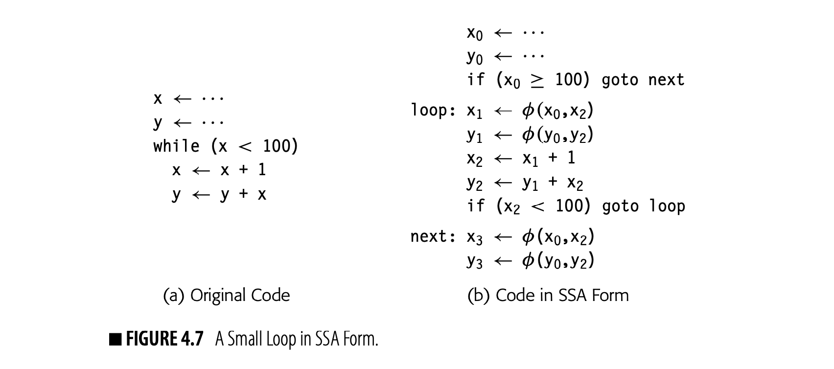
The code shape for the loop is discussed in Section 7.5.2.

To clarify the impact of these rules, consider the small loop shown in Fig. 4.7(a). Panel (b) shows the same code in SSA form. Variable names include subscripts to create a distinct name for each definition. $ϕ$ -functions have been inserted at points where multiple distinct values can reach the start of a block. Finally, the while construct has been rewritten at a lower level of abstraction to expose the fact that the initial test refers to x0 while the end-of-loop test refers to x2.

The $ϕ$ -function has an unusual semantics. It acts as a copy operation that selects, as its argument, the value that corresponds to the edge along which control entered the block. Thus, when control flows into the loop from the block above the loop, the $ϕ$ -functions at the top of the loop body copy the values of x0 and y0 into x1 and y1, respectively. When control flows into the loop from the test at the loop's bottom, the $ϕ$ -functions select their other arguments, x2 and y2.

The definition of SSA form prevents two $ϕ$ -functions from defining the same SSA name.

The execution semantics of $ϕ$ -functions are different than other operations. On entry to a block, all its $ϕ$ -functions read the value of their appropriate argument, in parallel. Next, they all define their target SSA names, in parallel. Defining their behavior in this way allows the algorithms that manipulate SSA form to ignore the ordering of $ϕ$ -functions at the top of a block--an important simplification. It does, however, complicate the process of translating SSA form back into executable code, as discussed in Section 9.3.5.

Lifetime For a value a, its lifetime spans from its first definition to its last use.

SSA form was intended for analysis and optimization. The placement of φ-functions in SSA form encodes information about the creation and use of individual values. The single-assignment property of the name space al- lows the compiler to ignore many issues related to the lifetimes of values;

BUILDING SSA Static single-assignment form is the only IR we describe that does not have an obvious construction algorithm. Section 9.3 presents one construction algorithm in detail. However, a sketch of the construction process will clarify some of the issues. Assume that the input program is already in ILOC form. To convert it to an equivalent linear form of SSA, the compiler must first insert $ϕ$ -functions and then rename the ILOC virtual registers.

The simplest way to insert $ϕ$ -functions is to find each block that has multiple CFG predecessors and add a $ϕ$ -function for each ILOC virtual register at the start of that block. This process inserts many unneeded $ϕ$ -functions; most of the complexity in the full algorithm focuses on eliminating those extraneous $ϕ$ -functions.

To rename the ILOC virtual registers, the compiler can process the blocks, in a depth-first order. For each virtual register, it keeps a counter. When the compiler encounters a definition of $r_{i}$ , it increments the counter for $r_{i}$ , say to k, and rewrites the definition with the name $r_{i_{k}}$ . As the compiler traverses the block, it rewrites each use of $r_{i}$ with $r_{i_{k}}$ until it encounters another definition of $r_{i}$ . (That definition bumps the counter to $k + 1$ .) At the end of a block, the compiler looks down each control-flow edge and rewrites the appropriate $ϕ$ -function parameter for $r_{i}$ in each block that has multiple predecessors.

After renaming, the code conforms to the two rules of SSA form. Each definition creates a unique name. Each use refers to a single definition. Several better SSA construction algorithms exist; they insert fewer \phi-functions than this simple approach.

for example, because names are not redefined, the value of a name is available along any path that proceeds from that operation. These two properties simplify and improve many optimizations.

The example exposes some oddities of SSA form that bear explanation. Consider the $ϕ$ -function that defines $x_{1}$ . Its first argument, $x_{0}$ , is defined in the block that precedes the loop. Its second argument, $x_{2}$ , is defined later in the block labeled loop. Thus, when the $ϕ$ first executes, one of its arguments is undefined. In many programming-language contexts, this would cause problems. Since the $ϕ$ -function reads only one argument, and that argument corresponds to the most recently taken edge in the CFG, it can never read the undefined value.

A $ϕ$ -function takes an arbitrary number of operands. To fit SSA form into a three-address ir, the compiler writer must include mechanisms to accommodate longer operand lists and to associate those operands with specific 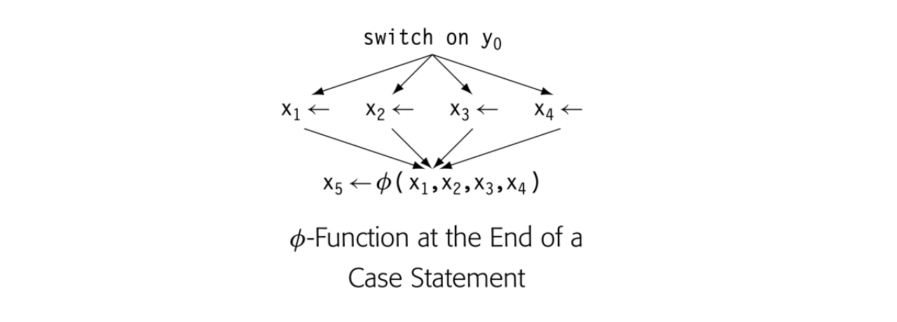The $ϕ$ -function for $x_{5}$ must have an argument for each case. The number of arguments it needs is bounded only by the number of paths that enter the block. Thus, an operation to represent that $ϕ$ -function in a linear IR will need an arbitrary number of arguments. It does not fit directly into the fixed-arity, three-address scheme.

In a simple array representation for three-address code, the compiler writer will need a side data structure to hold $ϕ$ -function arguments. In the other two schemes for implementing three-address code shown in Fig. 4.5, the compiler can insert tuples of varying size. For example, the tuples for load and load immediate might have space for just two names, while the tuple for a $ϕ$ -operation could be large enough to accommodate all its operands, plus an operand count.

SECTION REVIEW The compiler must generate internal names for all the values computed in a program. Those names may be explicit or implicit. The rules used to generate names directly affect the compiler’s ability to analyze and optimize the IR. Careful use of names can encode and expose facts for later use in optimization. Proliferation of names enlarges data structures and slows compilation.

The SSA name space encodes properties that can aid in analysis and optimization; for example, it lets optimizations avoid the need to reason about redefinitions of names (see Section 8.4.1). This additional precision in naming can both simplify algorithms and improve the optimizer’s results.

REVIEW QUESTIONS

The ILOC code shown in the margin on page 193 uses as many virtual register names as practical-assuming that $r_{i}$ and $r_{j}$ cannot be renamed because they represent variables in the program. Construct an equivalent code that uses as few virtual names as possible.

Convert the code shown in the margin to SSA form, following the explanation on page 195 . Does each $ϕ$ -functions that you inserted serve a purpose?

4.7 Placement of Values in Memory

Almost every ir has an underlying storage map. The compiler must assign a storage location to each value that the compiled code computes or uses. That location might be in a register or in memory. It might be a specific location: a physical register or (base address.offset) pair. It might be a symbolic location: a virtual register or a symbolic label. The location's lifetime must match the lifetime of the value; that is, it must be available and dedicated to the value from the time the value is created until the time of its last use.

This section begins with a discussion of memory models--the implicit rules used to assign values to data areas. The later subsections provide more detail on data area assignment and layout.

4.7.1 Memory Models

Before the compiler can translate the source program into its IR form, the compiler must understand, for each value computed in the code, where that value will reside. The compiler need not enumerate all the values and their locations, but it must have a mechanism to make those decisions consistently and incrementally as translation proceeds. Typically, compiler writers make a set of decisions and then apply them throughout translation. Together, these rules form a memory model for the compiled code.

Memory models help define the underlying model of computation: where does an operation find its arguments? They play a critical role in determining which problems the compiler must solve and how much space and time it will take to solve them.

Active value A value is active in the immediate neigh- borhood where it is used or defined.

Three memory models are common: a memory-to-memory model, a register-to-register model, and a stack model. These models share many characteristics; they differ in where they store values that are active in the current computation.

Memory-to-Memory Model Values have their primary home in memory. Either the IR supports memory-to-memory operations, or the code moves active values into registers and inactive values back to memory.

Register-to-Register Model Whenever possible, values are kept in a virtual register; some local, scalar values have their only home in a virtual register. Global values have their homes in memory (see Section 4.7.2).

Stack Model Values have their primary home in memory. The compiler moves active values onto and off of the stack with explicit operations (e.g., push and pop). Stack-based IRs and ISAs often include operations to reorder the stack (e.g., swap).

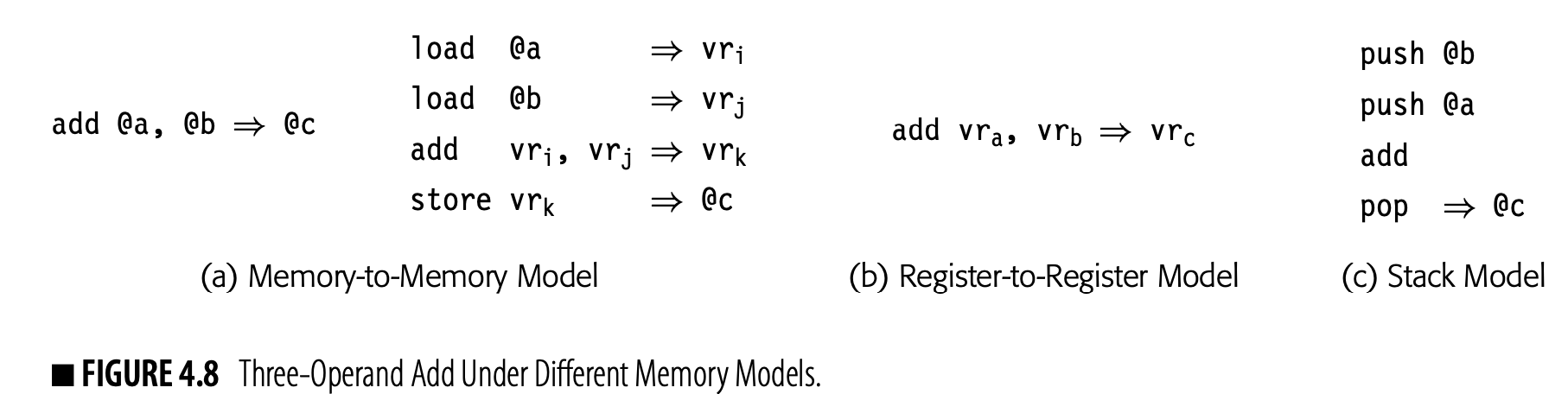
Unambiguous value A value that can be accessed with just one name is unambiguous.

Ambiguous value Any value that can be accessed by multiple names is ambiguous.

Fig. 4.8 shows the same add operation under each of these models. Panel (a) shows the operation under two different assumptions. The left column assumes that the add takes memory operands, shown as symbolic labels. The right column assumes that the add is a register-to-register operation, with values resident in memory. The choice between these two designs probably depends on the target machine's ISA. Panel (b) shows the same add in a register-to-register model. It assumes that a, b, and c are all unambiguous scalar values that reside in virtual registers: v $r_{a}$ , v $r_{b}$ , and v $r_{c}$ , respectively. Panel (c) shows the operation under a stack model; it assumes that the variable's home locations are in memory and named by symbolic labels.

These distinct memory models have a strong impact on the shape of the IR code and on the priorities for the optimizer and back end.

In a memory-to-memory model, the unoptimized form of the code may use just a few registers. That situation places a premium on optimizations that promote values into unused registers for nontrivial parts of their lifetimes. In the back end, register allocation focuses more on mapping names than on reducing demand for physical registers.
In a register-to-register model, the unoptimized code may use many more virtual registers than the target machine supplies. That situation encourages optimizations that do not significantly increase demand for registers. In the back end, register allocation is required for correctness and is one of the key determiners of runtime performance.

The JAVA HotSpot server compiler trans- lated JAVA bytecode to a graphical IR for optimization and code generation.

In a stack model, the structure of the target machine becomes critical. If the ISA has stack operations, as does the JAVA virtual machine, then optimization focuses on improving the stack computation. If the ISA is a Cisc or RISC processor, then the compiler will likely translate the stack-machine code into some other form for code generation.

In the end, the choice of memory model has a strong influence on the design of the compiler's optimizer and back end.

The hierarchy of memory operations in ILOC 9X

Under any memory model, the compiler writer should look for ways to encode more facts about values into the IR. In the 1990s, we built a research compiler that used an IR named ILOC 9x. The IR featured a hierarchy of memory operations that allowed the compiler to encode knowledge about values kept in memory. At the bottom of the hierarchy, the compiler had little or no knowledge about the value; at the top of the hierarchy, it knew the actual value. These operations are as follows:

Operation	Meaning
Immediate load Nonvarying load	Loads a known constant value into a register. Loads a value that does not change at runtime. The compiler does not know the value but can prove that the program does not change it.
Scalar load & store	Operate on a scalar value, not an array element, a structure element, or a pointer-based value.
Generic load & store	Operate on a value that may vary and may be non- scalar. It is the general-case operation.

With this hierarchy, the front end encoded knowledge about the target value directly into the ILOC 9x code. Other passes could rewrite operations from a more general to a more restricted form as they discovered new facts. For example, if the compiler discovered that a load always produced a known constant value, it replaced the generic or scalar load with an immediate load.

Optimizations capitalized on the facts encoded in this way. For example, a comparison between the result of a nonvarying load and a constant must itself be invariant—a fact that might be difficult or impossible to prove with a generic load operation.

4.7.2 Keeping Values in Registers

Spill

A register allocator spills a value by storing it to a designated location in memory. It may later restore the value to a register.

With a register-to-register memory model, the compiler tries to assign as many values as possible to virtual registers. This approach relies heavily on the register allocator to map virtual registers in the IR to physical registers in the final code, and to spill to memory any virtual register that it cannot keep in a physical register.

The compiler cannot keep an ambiguous value in a register across an assignment. With an unambiguous value $x$ , the compiler knows precisely where $x$ 's value changes: at assignments to $x$ . Thus, the compiler can safely generate code that keeps $x$ in a register.

With an ambiguous value $x$ , however, an assignment to some other ambiguous value $y$ might change $x$ 's value. If the compiler tries to hold $x$ in a register across an assignment to $y$ , the register may not be updated with the new value. To make matters worse, in a given procedure, $x$ and $y$ might refer to the same storage location in some invocations and not in others. This situation makes it difficult for the compiler to generate correct code that keeps $x$ in a register. Relegating $x$ to memory lets the addressing hardware resolve which assignments should change $x$ and which should not.

If a call passes a global name to a call-by- reference parameter, the callee can access the value with either its global name or the formal parameter name. The same effect occurs when a call passes a name x in two different call-by-reference parameter slots.

In practice, compilers decide which values they consider unambiguous, and relegate all ambiguous values to storage in memory--one of the data areas or the heap--rather than in a register. Ambiguity can arise in multiple ways. Values stored in pointer-based variables are often ambiguous. Call-by-reference parameters can be ambiguous. Many compilers treat array-element values as ambiguous because the compiler cannot tell if two references, such as A[i,j] and A[m,n] can ever refer to the same element.

Typically, compilers focus on proving that a given value is unambiguous. The analysis might be cursory and local. For example, in C, any local variable whose address is never taken is unambiguous. More complex analyses build sets of possible names for each pointer variable; any variable whose set has just one element is unambiguous. Analysis cannot resolve all ambiguities; the unprovable cases are treated as if they were proven to be ambiguous.

Language features can affect the compiler's ability to analyze ambiguity. For example, ANSI C includes two keywords that directly communicate information about ambiguity. The restrict keyword informs the compiler that a pointer is unambiguous. It is often used when a procedure passes an address directly at a call site. The volatile keyword lets the programmer declare that the contents of a variable may change arbitrarily and without notice. It is used for hardware device registers and for variables that might be modified by interrupt service routines or other threads of control in an application.

4.7.3 Assigning Values to Data Areas

Data area A region in memory set aside to hold data values. Each data area is associated with some specific scope. Examples include local data areas for pro- cedures and global data areas.

Just as the compiler must choose a name for each value in the program, so, too, must it decide where those values will reside at runtime. While the memory model determines where values live while they are active, each of the memory models discussed in Section 4.7.1 consigns some values to memory when they are not active. The compiler must decide, for each such value, where it should reside during its lifetime.

Most temporary values will live in the space reserved for active values--either registers or memory locations in the local data area--as determined by both the memory model and the availability of space. For variables that are declared in the source program, the compiler assigns each one a permanent home, based on its individual properties: its lifetime, its visibility, and its declaring scope.

Lifetime A value's lifetime refers to the period of time during which its value can be defined or referenced. Outside of a value's lifetime, it is undefined.

Region of Visibility A value is visible if it can be named--that is, the code can read or write the value. Its region of visibility is, simply, the code in which it is visible.

Declaring Scope A variable's lifetime and visibility depend on the scope that declares it. For example, a file static variable in C has a lifetime of the entire execution; it is only visible inside the file that declares it.

Programming languages have rules that determine lifetime, visibility, and scope for each name.

To simplify memory management, most compilers create a set of data areas associated with various program scopes. For memory resident variables, the combination of lifetime, visibility, and declaring scope determines which data area will hold the variable's value.

From a storage layout perspective, the compiler will categorize lifetimes into one of three categories.

Automatic A name whose lifetime matches a single activation of the scope that declares it is an automatic variable.

Automatic An automatic variable's lifetime matches one activation of its scope (a procedure or block). The value is defined and used inside the scope and its value ceases to exist on exit from the scope. A local variable is, typically, automatic by default.

We call these variables "automatic" because their allocation and deallocation can be handled as part of entry and exit for the corresponding scope. At runtime, each invocation of a procedure has its own local data area where automatic variables can be stored.

Static A name that retains its value across mul- tiple activations of its scope is a static variable.

Static A static variable's lifetime might span multiple activations of its declaring scope. If it is assigned a value, that value persists after control exists the scope where the assignment occurred.

The compiler can allocate such variables once, before execution; they are, in effect, always present. Static variables are stored in a preallocated data area associated with the declaring scope. The compiler may combine the static data areas for multiple scopes.

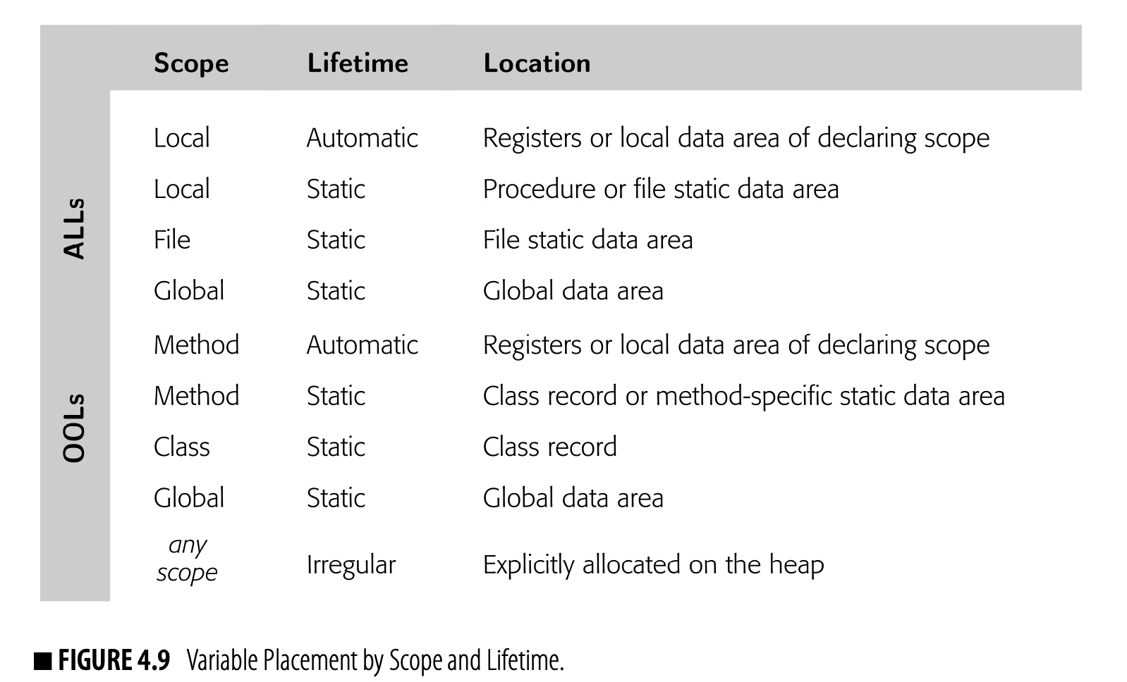
Constant values are a special case; they are static values that can be initialized with an assembly-level directive. The compiler typically creates a separate data area for them, often called a constant pool.

Irregular An entity whose lifetime depends on ex- plicit allocation and either explicit or implicit deallocation is an irregular entity.

Irregular An irregular variable has a lifetime that is not tied to any single scope. It is, typically, allocated explicitly; it may be freed either explicitly or implicitly. Examples include objects in JAVA and strings created with malloc in C.

Variables with irregular lifetimes are, in general, allocated space on the runtime heap (see Section 5.6.1).

The compiler can categorize each value by its lifetime and scope. This classification suggests a specific data area for the value's storage. Fig. 4.9 shows a typical scheme that a compiler might use to place variables into registers and data areas.

Given a mapping from values to data areas, the compiler must assign each memory-resident value a location. It iterates over the data areas and, within a data area, over the values for that data area. It assigns each value a specific offset from the start of the data area. Algorithms for this assignment are discussed in Section 5.6.3.

For values that might be kept in registers, the compiler assigns them a virtual register name. The actual assignment of virtual registers to hardware registers is left to the register allocator.

SECTION REVIEW The compiler must determine, for each value that the program computes, where that value will reside at runtime. The compiler determines those locations based on the programming language, on the memory model adopted by the compiler, on lifetime information for the values, and on the compiler writer’s knowledge of the target machine’s system architecture. The compiler systematically assigns each value to a register or a data area and assigns offsets within data areas to individual values. Decisions about the placement of values can affect the performance of compiled code. Storage layout can change the locality behavior of the program. Storage assignment decisions can encode subtle knowledge about properties of the underlying code, such as the ambiguity of values.

REVIEW QUESTIONS

Consider the function fib shown in the margin. Write down the ILOC that a compiler’s front end might generate for this code using a register-to-register model and using a memory-to-memory model. How does the code for the two models compare?

Write the pseudocode for an algorithm that takes a list of variables assigned to some data area and assigns them offsets. Explain what in- formation the compiler needs for each variable.

4.8 Summary and Perspective

The choice of an IR has a major impact on the design, implementation, speed, and effectiveness of a compiler. None of the intermediate forms de- scribed in this chapter are, definitively, the right answer for all compilers or all tasks in a given compiler. The compiler writer must consider the overall goals of a compiler project when selecting an IR, designing its im- plementation, and adding ancillary data structures such as symbol and label tables.

Contemporary compiler systems use all manner of IRs, ranging from parse trees and abstract syntax trees (often used in source-to-source systems) through lower-than-machine-level linear codes (used, for example, in GCC). Many compilers use multiple IRs—building a second or third one to per- form a particular analysis or transformation, then modifying the original, and definitive, one to reflect the result.

Chapter Notes

The literature on IRs and experience with them is sparse. Nonetheless, IRs have a major impact on both the structure and behavior of a compiler. The classic IR forms, such as syntax trees, ASTs, DAGs, quadruples, triples, and one-address code have been described in textbooks since the 1970s [8, 36,157,181]. New IR forms like SSA[56,120,279] are described in the literature on analysis and optimization. The original JAVA HotSpot Server compiler used a form of program dependence graph as its definitive IR[92]. Muchnick discusses IRs in detail and highlights the use of multiple levels of IR in a single compiler [279].

The observation that multiple passes over the code can lead to more efficient code dates back to Floyd [160]; this fundamental observation creates the need for IR and justifies the added expense of the multipass compiler. This insight applies in many contexts within a compiler.

The idea of using a hash function to recognize textually identical operations dates back to Ershov [150]. Its specific application in Lisp systems seems to appear in the early 1970s [135,174]; by 1980, it was common enough that McCarthy mentions it without citation [267].

Cai and Paige introduced multiset discrimination as an alternative to hashing [71]. Their intent was to create an efficient lookup mechanism with guaranteed constant time behavior. Closure-free regular expressions, described in Section 2.6.2, can achieve a similar effect. The work on shrinking the size of $R^{n}$ 's AST was done by David Schwartz and Scott Warren.

Exercises

Section 4.3

Both a parse tree and an abstract syntax tree retain information about the form of the source program.
What is the relationship between the size of the parse tree and the size of the input program?
What is the relationship between the size of the abstract syntax tree and the size of the input program?
What relationship would you expect between the size of the parse tree and the size of the abstract syntax tree? In other words, what value would you expect for $\frac{∣ p a rse t ree ∣}{∣ ab s t r a c t sy n t a x t ree ∣}$ ?
Write an algorithm to convert an expression tree into a DAG.

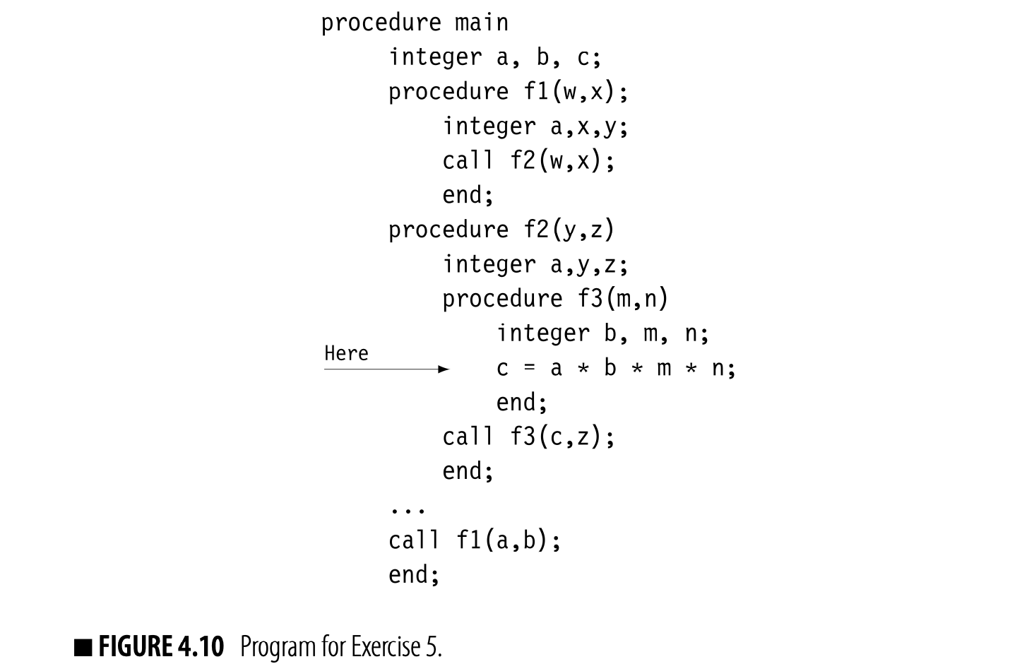3. Consider the following code fragment. Show how it might be repre- sented in an abstract syntax tree, in a control-flow graph, and in three- address code. 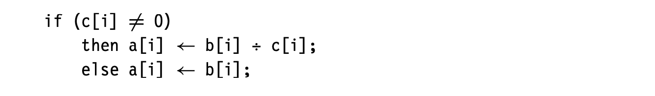Discuss the advantages of each representation. For what applications would one representation be preferable to the others?

The algorithm for constructing a CFG, shown in Fig. 4.6, assumes that the conditional branch operation, cbr, specifies a label for both the taken branch and the fall-through branch. Modify both FindLeaders and BuildGraph to handle input code where the cbr operation only specifies the taken branch.
You are writing a compiler for a simple lexically scoped language. Con- sider the example program shown in Fig. 4.10.
Draw the symbol table and its contents just before the line of code indicated by the arrow.
For each name mentioned in the statement indicated by the arrow, show which declaration defines it.
Consider the code fragment shown in Fig. 4.11. Draw its CFG.

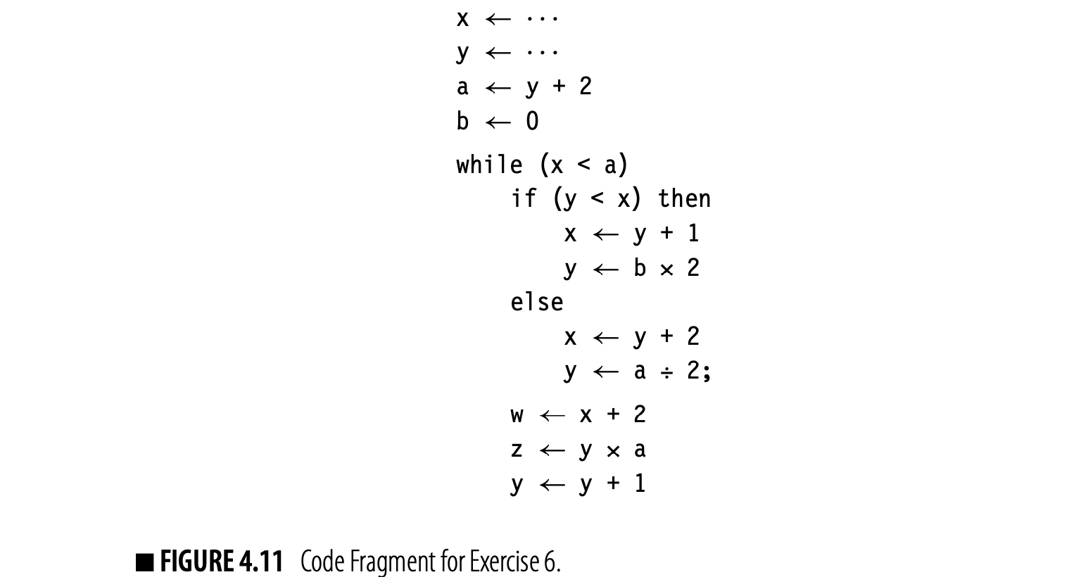
Section 4.6

Write both three-address code and stack-machine code to evaluate the expression $a \times (b + c) \div d$ . Assume that the ir can represent a load of a's value with a load from the label @a.

How many names does the three-address code use?
How many names does the stack-machine code use?

Three-address code and two-address code differ in the ways that the operations interact with the name space. With three-address code, overwriting a value in some name $n$ is a choice. With two-address code, ordinary arithmetic operations such as add overwrite one of the two arguments. Thus, with two-address code, the compiler must choose which operands to preserve and which operands to overwrite. Write down three ways that the compiler might encode the expression a $\leftarrow$ b x c into a low-level two-address code. Assume that b and c reside in $r_{b}$ and $r_{c}$ before the multiply operation. How might the compiler choose between these different encodings of the operation into two-address code?

Section 4.7

Consider the three C procedures shown in Fig. 4.12.

In a compiler that uses a register-to-register memory model, which variables in procedures A, B, and C would the compiler be forced to store in memory? Justify your answer.
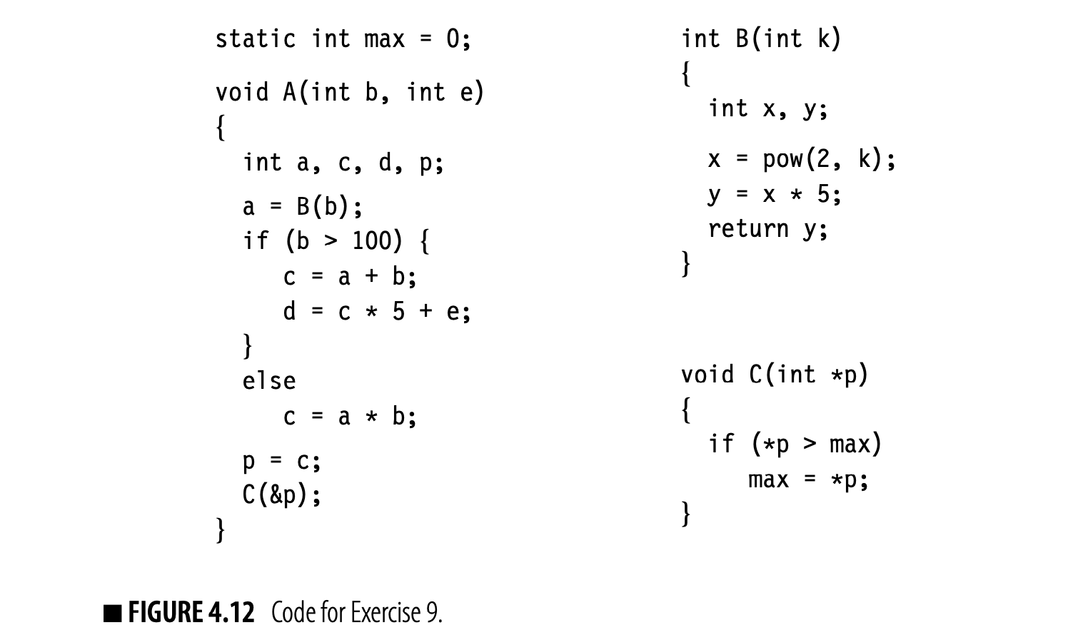
Suppose the compiler uses a memory-to-memory model. Consider the execution of the two statements that are in the if clause of the if-else construct. If the compiler has two registers available at that point in the computation, how many loads and stores would the compier need to issue in order to load values in registers and store them back to memory during execution of those two statements? What if the compiler has three registers available?

In FORTRAN, two variables can be forced to begin at the same storage location with an equivalence statement. For example, the following statement forces a and b to share storage:

Can the compiler keep a local variable in a register throughout the procedure if that variable appears in an equivalence statement? Justify your answer.

Chapter 5. Syntax-Driven Translation

5.1 Introduction

Fundamentally, the compiler is a program that reads in another program, builds a representation of its meaning, analyzes and improves the code in that form, and translates the code so that it executes on some target machine. Translation, analysis, optimization, and code generation require an in-depth understanding of the input program. The purpose of syntax-driven translation is to begin to assemble the knowledge that later stages of compilation will need.

As a compiler parses the input program, it builds an IR version of the code. It annotates that IR with facts that it discovers, such as the type and size of a variable, and with facts that it derives, such as where it can store each value. Compilers use two mechanisms to build the IR and its ancillary data structures: (1) syntax-driven translation, a form of computation embedded into the parser and sequenced by the parser's actions, and (2) subsequent traversals of the IR to perform more complex computations.

Conceptual Roadmap

The primary purpose of a compiler is to translate code from the source language into the target language. This chapter explores the mechanism that compiler writers use to translate a source-code program into an IR program. The compiler writer plans a translation, at the granularity of productions in the source-language grammar, and tools execute the actions in that plan as the parser recognizes individual productions in the grammar. The specific sequence of actions taken at compile time depends on both the plan and the parse.

During translation, the compiler develops an understanding, at an operational level, of the source program's meaning. The compiler builds a model of the input program's name space. It uses that model to derive information about the type of each named entity. It also uses that model to decide where, at runtime, each value computed in the code will live. Taken together, these facts let the compiler emit the initial IR program that embodies the meaning of the original source code program.

A Few Words About Time

Translation exposes all of the temporal issues that arise in compiler construction. At design time, the compiler writer plans both runtime behavior and compile-time mechanisms to create code that will elicit that behavior. She encodes those plans into a set of syntax-driven rules associated with the productions in the grammar. Still at design time, she must reason about both compile-time support for translation, in the form of structures such as symbol tables and processes such as type checking, and runtime support to let the code find and access values. (We will see that support in Chapters 6 and 7, but the compiler writer must think about how to create, use, and maintain that support while designing and implementing the initial translation.)

Runtime system the routines that implement abstractions such as the heap and I/O

At compiler-build time, the parser generator turns the grammar and the syntax-driven translation rules into an executable parser. At compile time, the parser maps out the behaviors and bindings that will take effect at run- time and encodes them in the translated program. At runtime, the compiled code interacts with the runtime system to create the behaviors that the com- piler writer planned back at design time.

Overview

The compiler writer creates a tool--the compiler--that translates the input program into a form where it executes directly on the target machine. Thecompiler, then, needs an implementation plan, a model of the name space, and a mechanism to tie model manipulation and IR generation back to the structure and syntax of the input program. To accomplish these tasks:

The compiler needs a mechanism that ties its information gathering and IR-building processes to the syntactic structure and the semantic details of the input program.
The compiler needs to understand the visibility of each name in the code--that is, given a name $x$ , it must know the entity to which $x$ is bound. Given that binding, it needs complete type information for $x$ and an access method for $x$ .
The compiler needs an implementation scheme for each programming language construct, from a variable reference to a case statement and from a procedure call to a heap allocation.

This chapter focuses on a mechanism that is commonly used to specify syntax-driven computation. The compiler writer specifies actions that should be taken when the parser reduces by a given production. The parser generator arranges for those actions to execute at the appropriate points in the parse. Compiler writers use this mechanism to drive basic information gathering, IR generation, and error checking at levels that are deeper than syntax (e.g., does a statement reference an undeclared identifier?).

Chapters 6 and 7 discuss implementation of other common programming language constructs.

Section 5.3 introduces a common mechanism used to translate source code into IR. It describes, as examples, implementation schemes for expression evaluation and some simple control-flow constructs. Section 5.4 explains how compilers manage and use symbol tables to model the naming environment and track the attributes of names. Section 5.5 introduces the subject of type analysis; a complete treatment of type systems is beyond the scope of this book. Finally, Section 5.6 explores how the compiler assigns storage locations to values.

5.2 BACKGROUND

The compiler makes myriad decisions about the detailed implementation of the program. Because the decisions are cumulative, compiler writers often adopt a strategy of progressive translation. The compiler's front end builds an initial IR program and a set of annotations using information available in the parser. It then analyzes the IR to infer additional information and refines the details in the IR and annotations as it discovers and infers more information.

To see the need for progressive translation, consider a tree representation of an array reference $a [i, j]$ . The parser can easily build a relatively abstract IR, such as the near-source AST shown in the margin. The AST only encodes facts that are implicit in the code's text. 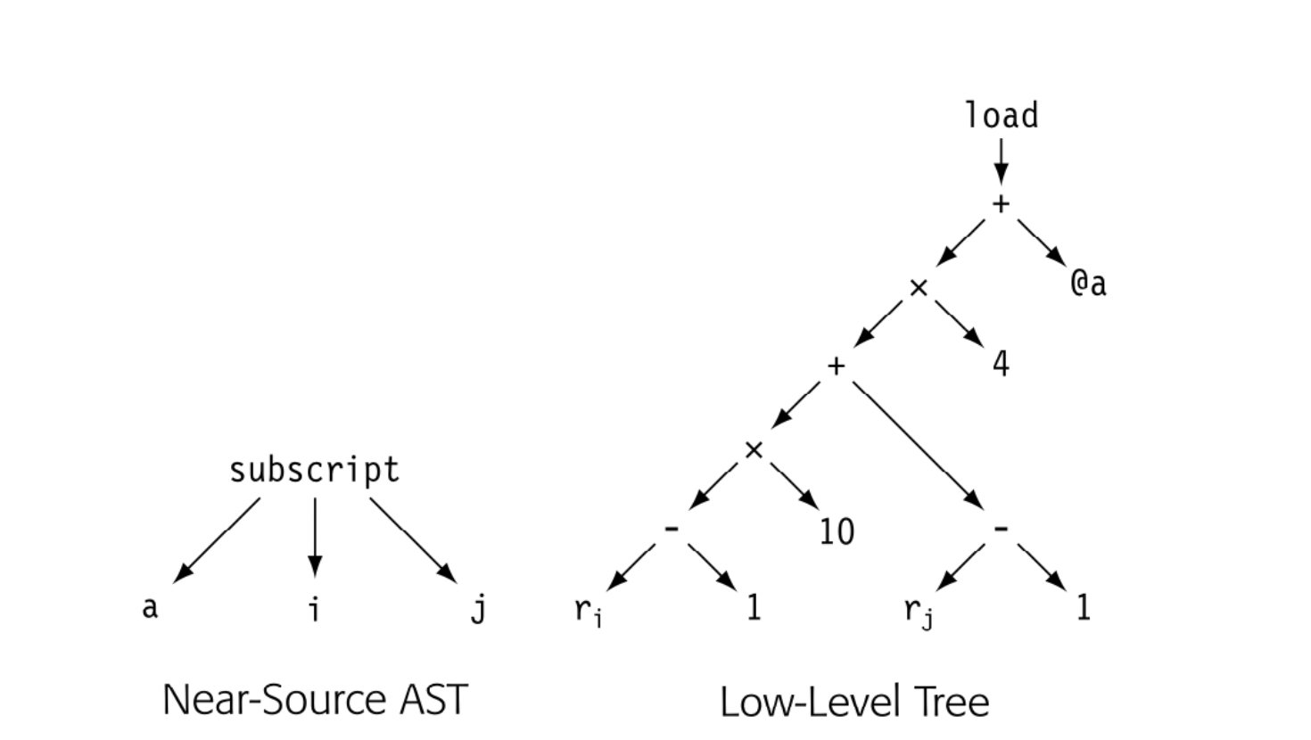To generate assembly code for the reference, the compiler will need much more detail than the near-source AST provides. The low-level tree shown in the margin exposes that detail and reveals a set of facts that cannot be seen in the near-source tree. All those facts play a role in the final code.

The compiler must know that a is a $10 \times 10$ array of four-byte integers with lower bounds of 1 in each dimension. Those facts are derived from the statements that declare or create a.
The compiler must know that a is stored in row-major order (see Fig. 5.16). That fact was decided by the language designer or the compiler writer before the compiler was written.
The compiler must know that @a is an assembly-language label that evaluates to the runtime address of the first element of a (see Section 7.3). That fact derives from a naming strategy adopted at design time by the compiler writer.

To generate executable code for a[i,j], the compiler must derive or develop these facts as part of the translation process.

This chapter explores both the mechanism of syntax-driven translation and its use in the initial translation of code from the source language to IR. The mechanism that we describe was introduced in an early LR(1) parser generator, yacc. The notation allows the compiler writer to specify a small snippet of code, called an action, that will execute when the parser reduces by a specific production in the grammar.

Syntax-driven translation lets the compiler writer specify the action and relies on the parser to decide when to apply that action. The syntax of the input program determines the sequence in which the actions occur. The actions can contain arbitrary code, so the compiler writer can build and maintain complex data structures. With forethought and planning, the compiler writer can use this syntax-driven translation mechanism to implement complex behaviors.

Through syntax-driven translation, the compiler develops knowledge about the program that goes beyond the context-free syntax of the input code. Syntactically, a reference to a variable $x$ is just a name. During translation, the compiler discovers and infers much more about $x$ from the contexts in which the name appears.

The source code may define and manipulate multiple distinct entities with the name $x$ . The compiler must map each reference to $x$ back to the appropriate runtime instance of $x$ ; it must bind $x$ to a specific entity based on the naming environment in which the reference occurs. To do so, it builds and uses a detailed model of the input program's name space.
Once the compiler knows the binding of $x$ in the current scope, it must understand the kinds of values that $x$ can hold, their size and structure, and their lifetimes. This information lets the compiler determine what operations can apply to $x$ , and prevents improper manipulation of $x$ . This knowledge requires that the compiler determine the type of $x$ and how that type interacts with the contexts in which $x$ appears.
To generate code that manipulates $x$ 's value, the compiler must know where that value will reside at runtime. If $x$ has internal structure, as with an array, structure, string, or record, the compiler needs a formula to find and access individual elements inside $x$ . The compiler must determine, for each value that the program will compute, where that value will reside.

To complicate matters, executable programs typically include code compiled at different times. The compiler writer must design mechanisms that allow the results of the separate compilations to interoperate correctly and seamlessly. That process begins with syntax-driven translation to build an IR representation of the code. It continues with further analysis and refinement. It relies on carefully planned interactions between procedures and name spaces (see Chapter 6).

5.3 Syntax-Driven Translation

Syntax-driven translation is a collection of techniques that compiler writers use to tie compile-time actions to the grammatical structure of the input program. The front end discovers that structure as it parses the code. The compiler writer provides computations that the parser triggers at specific points in the parse. In an LR(1) parser, those actions are triggered when the parser performs a reduction.

5.3.1 A First Example

Fig. 5.1(a) shows a simple grammar that describes the set of positive integers. We can use syntax-driven actions tied to this grammar to compute the value of any valid positive integer.

Panel (b) contains the Action and Goto tables for the grammar. The parser has three possible reductions, one per production.

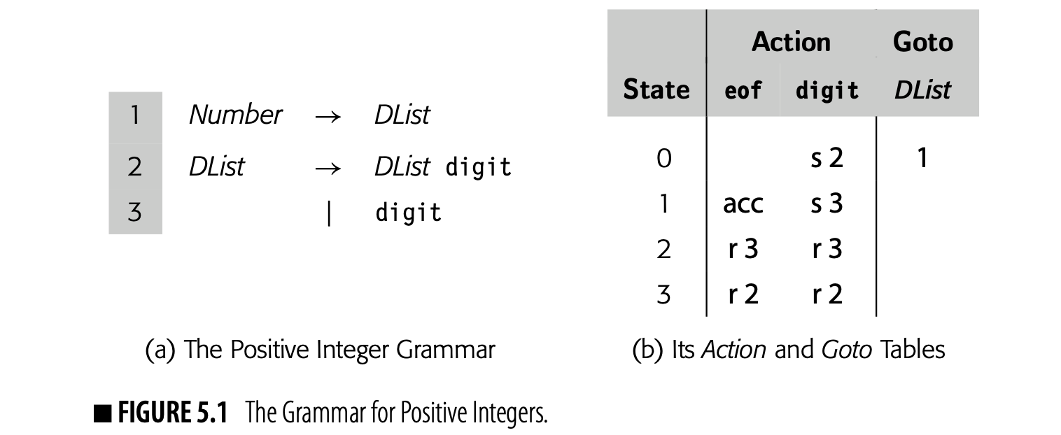
The parser reduces by rule 3, $DList \to digit$ , on the leftmost digit in the number.
The parser reduces by rule 2, $DList \to DList$ $digit$ , for each digit after the first digit.
The parser reduces by rule 1, $Number \to DList$ after it has already reduced the last digit.

The parser can compute the integer's value with a series of production-specific tasks. It can accumulate the value left to right and, with each new digit, multiply the accumulated value by ten and add the next digit. Values are associated with each symbol used in the parse. We can encode this strategy into production-specific rules that are applied when the parser reduces.

Using the notation popularized by the parser generators yacc and bison, the rules might be: The symbols $$ ，$1 and $2 refer to values associated with grammar symbols in the production. $$ refers to the nonterminal symbol on the rule's left-hand side (LHS). The symbol i refers to the value for the _i_th symbol on the rule's right-hand side (RHS).

The example assumes that CTo1() converts the character from the lexeme to an integer. The compiler writer must pay attention to the types of the stack cells represented by $$, $1, and so on.

Recall that the initial on the stack repre- sents the pair ⟨INVALID, INVALID⟩.

Using the Action and Goto tables from Fig. 5.1(b) to parse the string "175", an LR(1) parser would take the sequence of actions shown in Fig. 5.2. The reductions, in order, are: reduce 3, reduce 2, reduce 2, and accept.

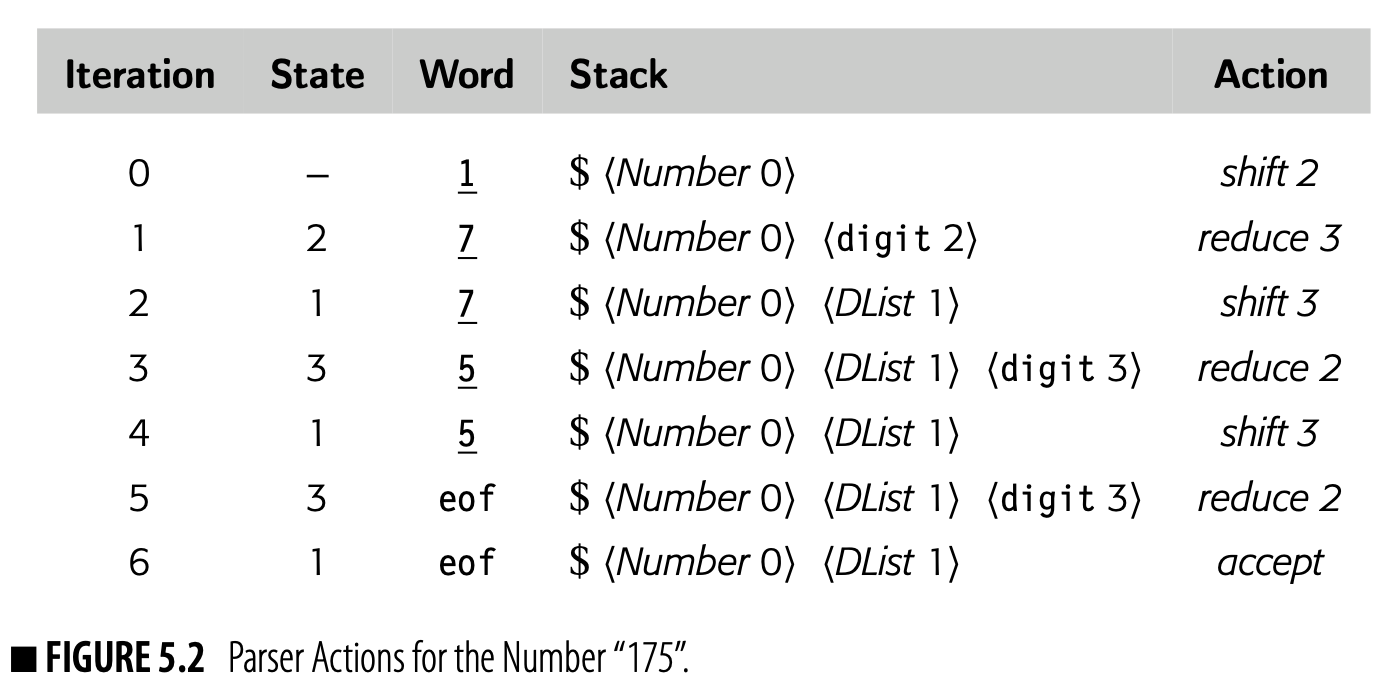
Reduce 3 applies rule 3's action with the integer 1 as the value of digit. The rule assigns one to the LHS_DList_.
Reduce 2 applies rule 2's action, with 1 as the RHS_DList_'s value and the integer 7 as the digit. It assigns $1 \times 10$ + $7$ = $17$ to the LHS_DList_.
Reduce 2 applies rule 2's action, with 17 as the RHS_DList_'s value and 5 as the digit. It assigns $17 \times 10$ + $5$ = $175$ to the LHS_DList_.
The accept action, which is also a reduction by rule 1, returns the value of the LHS_DList_, which is 175.

The reduction rules, applied in the order of actions taken by the parser, create a simple framework that computes the integer's value.

The critical observation is that the parser applies these rules in a predictable order, driven by the structure of the grammar and the parse of the input string. The compiler writer specifies an action for each reduction; the sequencing and application of those actions depend entirely on the grammar and the input string. This kind of syntax-driven computation forms a programming paradigm that plays a central role in translation and finds many other applications. 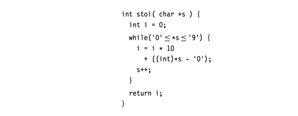Of course, this example is overkill. A real system would almost certainly perform this same computation in a small, specialized piece of code, similar to the one in the margin. It implements the same computation, without the overhead of the more general scanning and parsing algorithms. In practice, this code would appear inline rather than as a function call. (The call overhead likely exceeds the cost of the loop.) Nonetheless, the example works well for explaining the principles of syntax-driven computation.

An Equivalent Treewalk Formulation

These integer-grammar value computations can also be written as recursive treewalks over syntax trees. Fig. 5.3(a) shows the syntax tree for "175" with the left recursive grammar. Panel (b) shows a simple treewalk to compute its value. It uses "integer(c)" to convert a single character to an integer value.

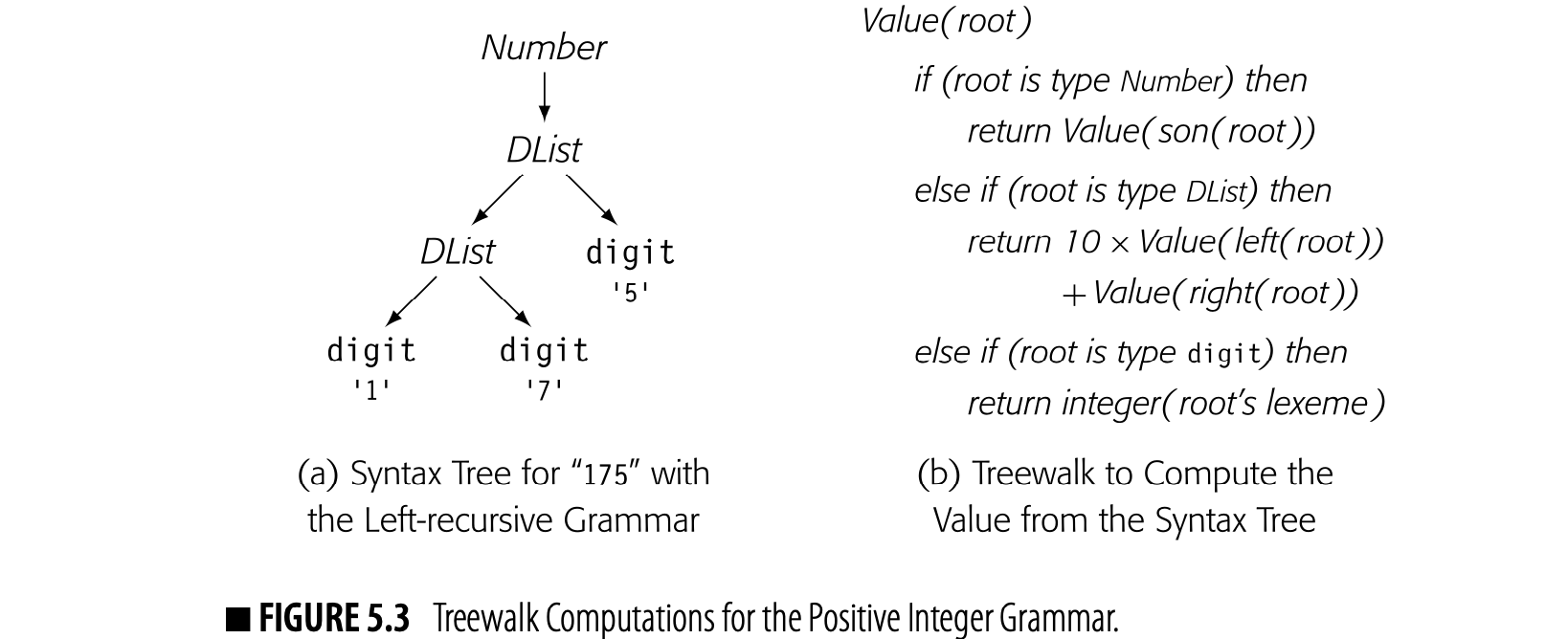
The treewalk formulation exposes several important aspects of yacc-style syntax-driven computation. Information flows up the syntax tree from the leaves toward the root. The action associated with a production only has names for values associated with grammar symbols named in the production. Bottom-up information flow works well in this paradigm. Top-down information flow does not.

The restriction to bottom-up information flow might appear problematic. In fact, the compiler writer can reach around the paradigm and evade these restrictions by using nonlocal variables and data structures in the "actions." Indeed, one use for a compiler's symbol table is precisely to provide nonlocal access to data derived by syntax-driven computations.

In principle, any top-down information flow problem can be solved with a bottom-up framework by passing all of the information upward in the tree to a common ancestor and solving the problem at that point. In practice, that idea does not work well because (1) the implementor must plan all the information flow; (2) she must write code to implement it; and (3) the computed result appears at a point in the tree far from where it is needed. In practice, it is often better to rethink the computation than to pass all of that information around the tree.

Form of the Grammar

Because the grammar dictates the sequence of actions, its shape affects the computational strategy. Consider a right-recursive version of the grammar for positive integers. It reduces the rightmost digit first, which suggests the following approach:

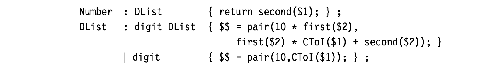
This scheme accumulates, right to left, both a multiplier and a value. To store both values with a DList, it uses a pair constructor and the functions first and second to access a pair's component values. While this paradigm works, it is much harder to understand than the mechanism for the left-recursive grammar.

In grammar design, the compiler writer should consider the kinds of computation that she wants the parser to perform. Sometimes, changing the grammar can produce a simpler, faster computation.

5.3.2 Translating Expressions

Expressions form a large portion of most programs. If we consider them as trees--that is, trees rather than directed acyclic graphs--then they are a natural example for syntax-driven translation. Fig. 5.4 shows a simple syntax-driven framework to build an abstract syntax tree for expressions. The rules are simple.

If a production contains an operator, it builds an interior node to represent the operator.
If a production derives a name or number, it builds a leaf node and records the lexeme.
If the production exists to enforce precedence, it passes the AST for the subexpression upward.

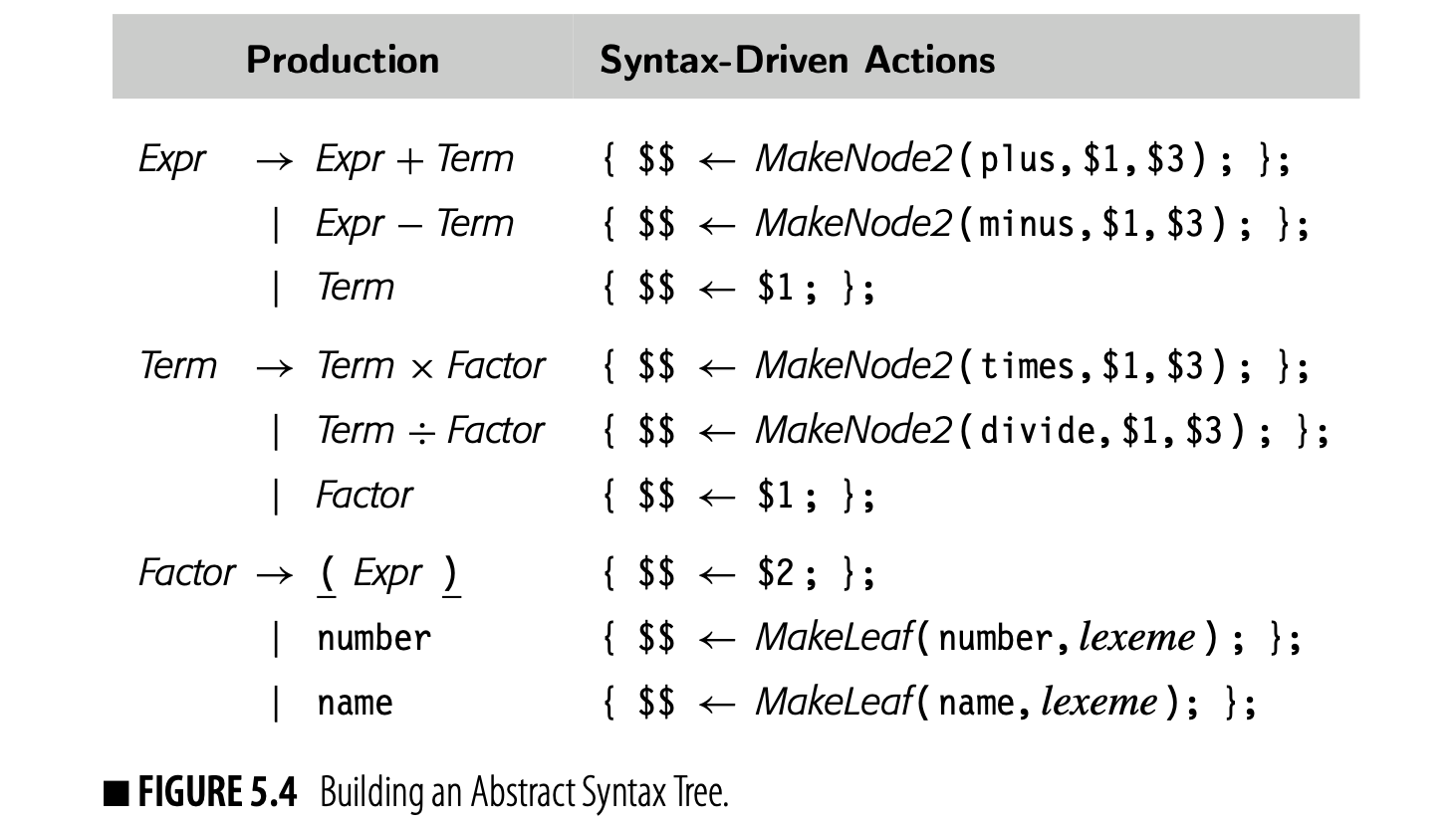
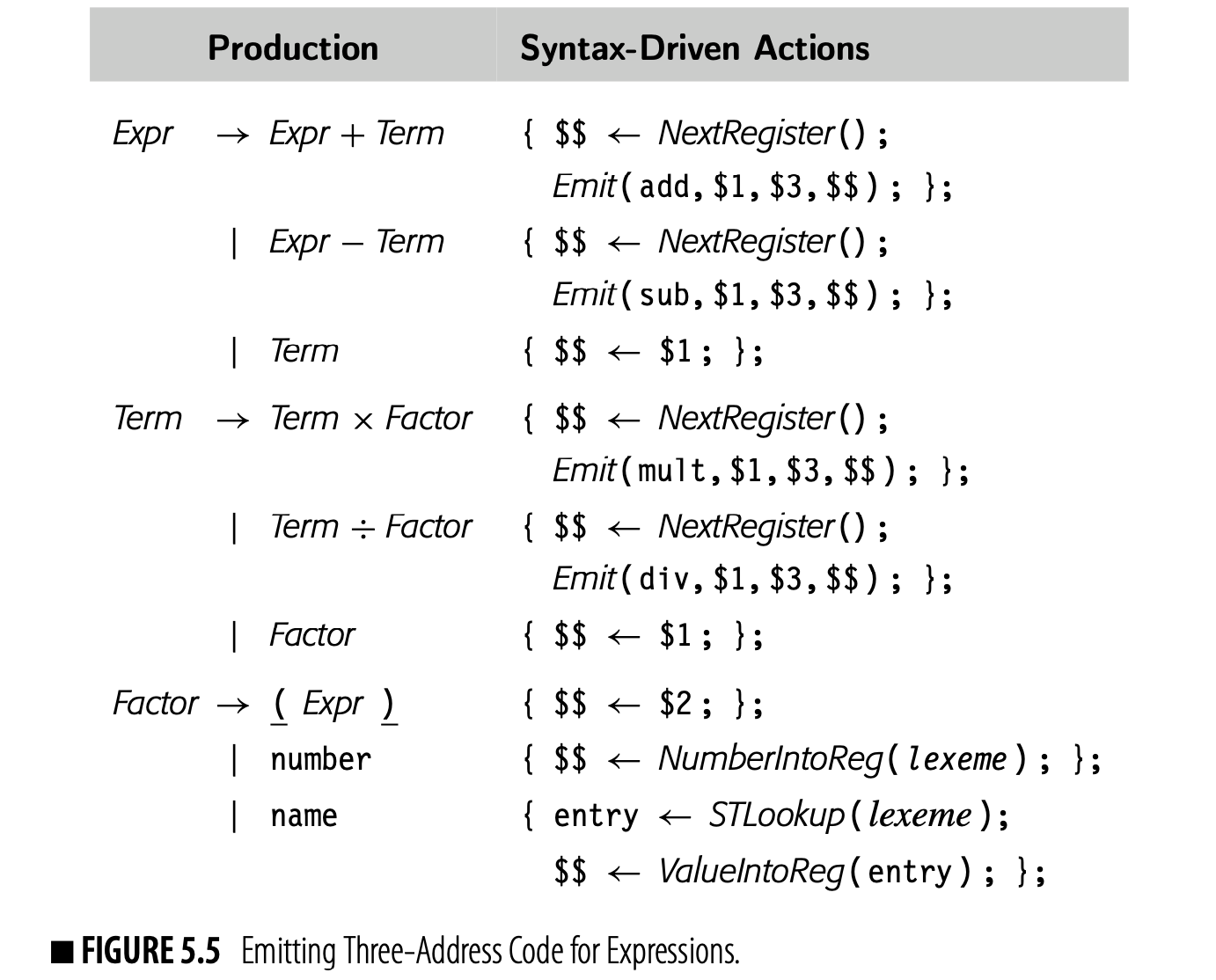
The code uses two constructors to build the nodes. $MakeNode2 (a, b, c)$ builds a binary node of type $a$ with children $b$ and $c$ . $MakeLeed (name, a)$ builds a leaf node and associates it with the lexeme $a$ . For the expression $a - 2 x b$ , this translation scheme would build the simple AST shown in the margin. ASTs have a direct and obvious relationship to the grammatical structure of the input program. Three-address code lacks that direct mapping. Nonetheless, a syntax-driven framework can easily emit three-address code for expressions and assignments. Fig. 5.5 shows a syntax-driven framework to emit $ILOC$ -like code from the classic expression grammar. The framework assumes that values reside in memory at the start of the expression.

To simplify the framework, the compiler writer has provided high-level functions to abstract away the details of where values are stored.

NextRegister returns a new register number.
NumberInfoReg returns the number of a register that holds the constant value from the lexeme.
STLookup takes a name as input and returns the symbol table entry for the entity to which the name is currently bound.
ValueIntoReg returns the number of a register that holds the current value of the name from the lexeme.

If the grammar included assignment, it would need a helper function RegIn- toMemory to move a value from a register into memory.

Helper functions such NumberIntoReg and ValueIntoReg must emit three- address code that represents the access methods for the named entities. If the IR only has low-level operations, as occurs in ILOC, these functions can become complex. The alternative approach is to introduce high-level oper- ations into the three-address code that preserve the essential information, and to defer elaboration of these operations until after the compiler fully understands the storage map and the access methods. Applying this syntax-driven translation scheme to the expression $a - 2 \times b$ produces the ILOC code shown in the margin. The code assumes that $r_{a r p}$ holds a pointer to the procedure's local data area and that $@a$ and $@b$ are the offsets from $r_{a r p}$ at which the program stores the values of a and b. The code leaves the result in $r_{5}$ .

Implementation in an LR(1) Parser

This style of syntax-driven computation was introduced in yacc, an early LALR(1) parser generator. The implementation requires two changes to the LR(1) skeleton parser. Understanding those changes sheds insight on both the yacc notation and how to use it effectively. Fig. 5.6 shows the modified skeleton LR(1) parser. Changes are typeset in bold typeface.

Parser generators differ in what value they assign to a terminal symbol.

The first change creates storage for the value associated with a grammar symbol in the derivation. The original skeleton parser stored its state in $⟨ sy mb o l, s t a t e ⟩$ pairs kept on a stack, where symbol was a grammar symbol and state was a parser state. The modified parser replaces those pairs with $⟨ sy mb o l, s t a t e, v a l u e ⟩$ triples, where value holds the entity assigned to $$$ in the reduction that shifted the triple onto the stack. Shift actions use the value of the lexeme.

The second change causes the parser to invoke a function called PerformActions before it reduces. The parser uses the result of that call in the value field when it pushes the new triple onto the stack.

The parser generator constructs PerformActions from the translation actions specified for each production in the grammar. The skeleton parser passes the function a production number; the function consists of a case statement that switches on that production number to the appropriate snippet of code for the reduction.

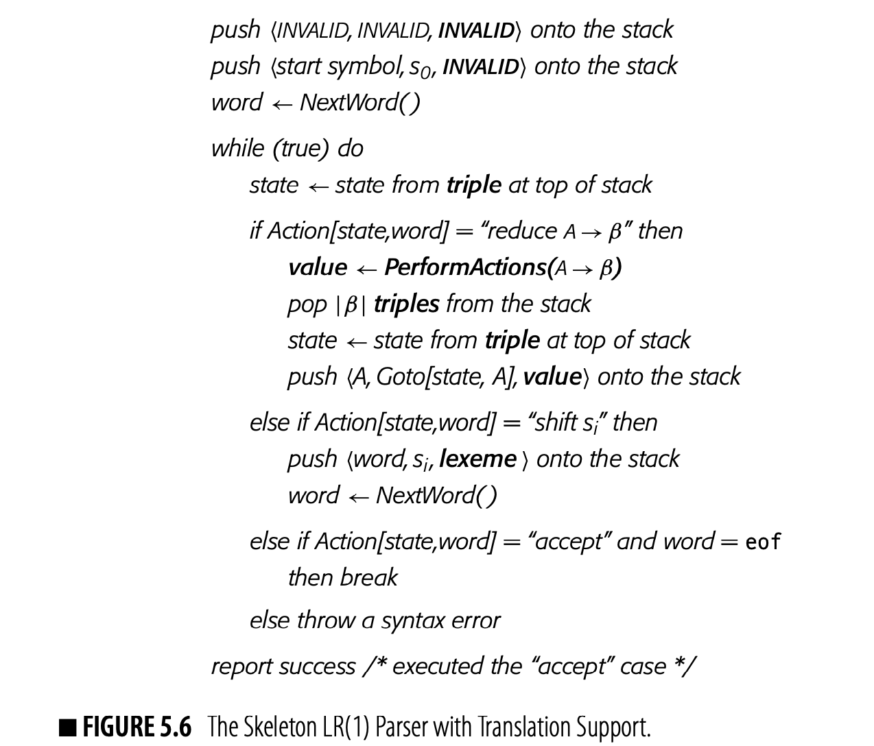
The remaining detail is to translate the yacc-notation symbols $$$, $1, $2$ , and so on into concrete references into the stack. $$$$ represents the return value for PerformActions. Any other symbol, $$ i$ , is a reference to the value field of the triple corresponding to symbol i in the production's RHS. Since those triples appear, in right to left order, on the top of the stack, $$ i$ translates to the value field for the triple located $∣ β ∣ - i$ slots from the top of the stack.

Handling Nonlocal Computation

The examples so far only show local computation in the grammar. Individual rules can only name symbols in the same production. Many of the tasks in a compiler require information from other parts of the computation; in a treewalk formulation, they need data from distant parts of the syntax tree.

Defining occurrence The first occurrence of a name in a given scope is its defining occurrence. Any subsequent use is a reference occurrence.

One example of nonlocal computation in a compiler is the association of type, lifetime, and visibility information with a named entity, such as a variable, procedure, object, or structure layout. The compiler becomes aware of the entity when it encounters the name for the first time in a scopethe name's defining occurrence. At the defining occurrence of a name x, the compiler must determine x's properties. At subsequent reference occurrences, the compiler needs access to those previously determined properties.

The use of a global symbol table to provide nonlocal access is analogous to the use of global variables in imperative programs.

The kinds of rules introduced in the previous example provide a natural mechanism to pass information up the parse tree and to perform local computation-between values associated with a node and its children. To translate an expression such as x+y into a low-level three-address IR, the compiler must access information that is distant in the parse tree--the declarations of x and y. If the compiler tries to generate low-level three-address code for the expression, it may also need access to information derived from the syntax, such as a determination as to whether or not the code can keep x in a register--that is, whether or not x is ambiguous. A common way to address this problem is to store information needed for nonlocal computations in a globally accessible data structure. Most compilers use a symbol table for this purpose (see Section 4.5).

The "symbol table" is actually a complex set of tables and search paths. Conceptually, the reader can think of it as a hashmap tailored to each scope. In a specific scope, the search path consists of an ordered list of tables that the compiler will search to resolve a name.

In a dynamically typed language such as PYTHON, statements that define x may change $x^{'} s$ attributes

Different parts of the grammar will manipulate the symbol table representation. A name's defining occurrence creates its symbol table entry. Its declarations, if present, set various attributes and bindings. Each reference occurrence will query the table to determine the name's attributes. Statements that open a new scope, such as a procedure, a block, or a structure declaration, will create new scopes and link them into the search path. More subtle issues may arise; if a C program takes the address of a variable a, as in 8a, the compiler should mark a as potentially ambiguous.

The same trick, using a global variable to communicate information between the translation rules, arises in other contexts. Consider a source language with a simple declaration syntax. The parser can create symbol-table entries for each name and record their attributes as it processes the declarations. For example, the source language might include syntax similar to the following set of rules: 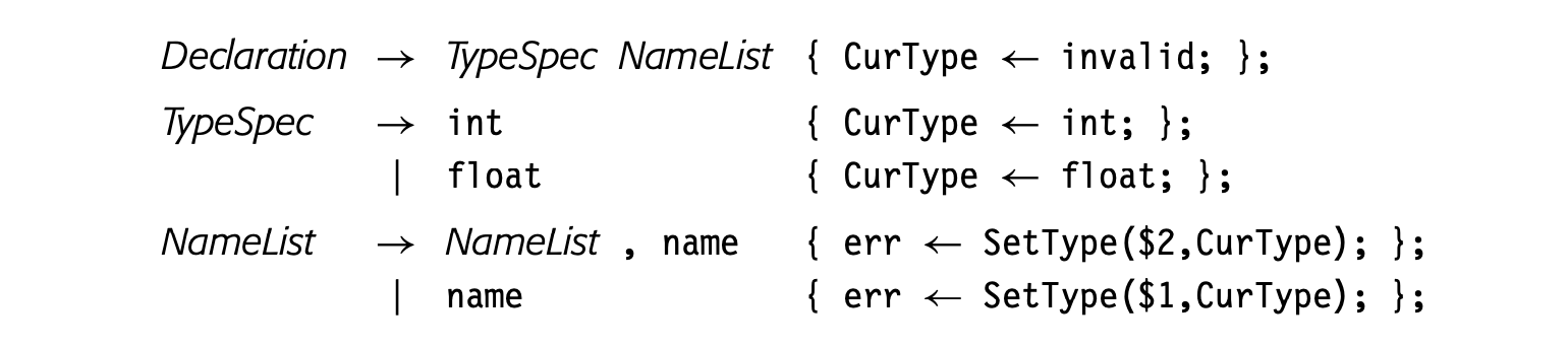where SetType creates a new entry for name if none exists and reports an error if name exists and has a designated type other than CurType.

The type of the declared variables is determined in the productions for _TypeSpec_. The action for _TypeSpec_ records the type into a global variable, CurType. When a name appears in the _NameList_ production, the action sets the name's type to the value in _CurType_. The compiler writer has reachedaround the paradigm to pass information from the RHS of one production to the RHS of another.

SINGLE-PASS COMPILERS

In the earliest days of compilation, implementors tried to build single-pass compilers—translators that would emit assembly code or machine code in a single pass over the source program. At a time when fast computers were measured in kiloflops, the efficiency of translation was an important issue.

To simplify single-pass translation, language designers adopted rules meant to avoid the need for multiple passes. For example, PASCAL requires that all declarations occur before any executable statement; this restriction allowed the compiler to resolve names and perform storage layout before emitting any code. In hindsight, it is unclear whether these restrictions were either necessary or desirable.

Making multiple passes over the code allows the compiler to gather more information and, in many cases, to generate more efficient code, as Floyd observed in 1961 [160]. With today’s more complex processors, almost all compilers perform multiple passes over an IR form of the code.

Form of the Grammar

The form of the grammar can play an important role in shaping the computation. To avoid the global variable CurType in the preceding example, the compiler writer might reformulate the grammar for declaration syntax as follows:

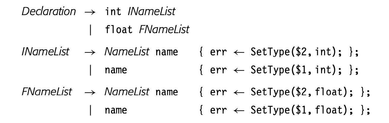
This form of the grammar accepts the same language. However, it creates distinct name lists for int and float names, As shown, the compiler writer can use these distinct productions to encode the type directly into the syntax-directed action. This strategy simplifies the translation framework and eliminates the use of a global variable to pass information between the productions. The framework is easier to write, easier to understand, and, likely, easier to maintain. Sometimes, shaping the grammar to the computation can simplify the syntax-driven actions.

Tailoring Expressions to Context

A more subtle form of nonlocal computation can arise when the compiler writer needs to make a decision based on information in multiple productions. For example, consider the problem of extending the framework in Fig. 5.5 so that it can emit an immediate multiply operation (mult1 in ILOC) when translating an expression. In a single-pass compiler, for example, it might be important to emit the mult1 in the initial IR. For the expression $a \times 2$ , the framework in Fig. 5.5 would produce something similar to the code shown in the margin. (The code assumes that a resides in $r_{a}$ .) The reduction by $Factor \to n u mb er$ emits the load1; it executes before the reduction by $Term \to Term \times Factor$ .

To recognize the opportunity for a mult1, the compiler writer would need to add code to the action for $Term \to Term \times Factor$ that recognizes when $3 co n t ain s a s ma ll in t e g erco n s t an t an d g e n er a t es t h e m u lt 1 in t ha t c a se . T h eco mm u t a t i v ec a se w o u l d re q u i re a s imi l a rc h ec k o n$ 1. Even with this effort, the load1 would remain. Subsequent optimization could remove it (see Section 10.2).

The fundamental problem is that the actions in our syntax-driven translation can only access local information because they can only name symbols in the current production. That structure forces the translation to emit the load1 before it can know that the value's use occurs in an operation that has an "immediate" variant. The obvious suggestion is to refactor the grammar to reflect the mult1 case. If the compiler writer rewrites $Term \to Term \times Factor$ with the three productions shown in the margin, then she can emit a mult1 in the action for $Term \to Term \times number$ , which will catch the case a x2. It will not, however, catch the case 2 x a. Forward substitution on the left operand will not work, because the grammar is left recursive. At best, forward substitution can expose either an immediate left operand or an immediate right operand.

The most comprehensive solution to this problem is to create the more general multiply operation and allow either subsequent optimization or instruction selection to discover the opportunity and rewrite the code. Either of the techniques for instruction selection described in Chapter 11 can discover the opportunity for mult1 and rewrite the code accordingly.

Peephole optimization an optimization that applies pattern match- ing to simplify code in a small buffer

If the compiler must generate the mult1 early, the most rational approach is to have the compiler maintain a small buffer of three to four operations and to perform peephole optimization as it emits the initial IR (see Section 11.3.1). It can easily detect and rewrite inefficiencies such as this one.

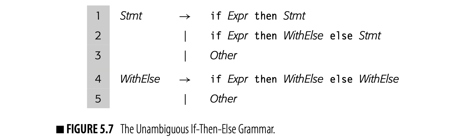
5.3.3 Translating Control-Flow Statements

As we have seen, the IR for expressions follows closely from the syntax for expressions, which leads to straightforward translation schemes. Control-flow statements, such as nested if-then-else constructs or loops, can require more complex representations.

Building an AST

The parser can build an AST to represent control-flow constructs in a natural way. Consider a nest of if-then-else constructs, using the grammar from Fig. 5.7. The AST can use a node with three children to represent the if. One child holds the control expression; another holds the statements in the then clause; the third holds the statements in the else clause. The drawing in the margin shows the AST for the input: The actions to build this AST are straightforward.

Building Three-Address Code

To translate an if-then-else construct into three-address code, the compiler must encode the transfers of control into a set of labels, branches, and jumps. The three-address IR resembles the obvious assembly code for the construct:

evaluate the control expression;
branch to the then subpart (s1) or the else subpart (s2) as appropriate;
at the end of the selected subpart, jump to the start of the statement that follows the if-then-else construct-the "exit."

This translation scheme requires labels for the then part, the else part, and the exit, along with a branch and two jumps.

Production 4 in the grammar from Fig. 5.7 shows the issues that arise in a translation scheme to emit ILOC-like code for an if-then-else. Other productions will generate the IR to evaluate the Expr and to implement the then and else parts. The scheme for rule 4 must combine these disjoint parts into code for a complete if-then-else.

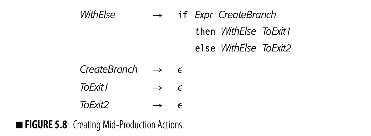The complication with rule 4 lies in the fact that the parser needs to emit IR at several different points: after the Expr has been recognized, after the WithElse in the then part has been recognized, and after the WithElse in the else part has been recognized. In a straightforward rule set, the action for rule 4 would execute after all three of those subparts have been parsed and the IR for their evaluation has been created.

The scheme for rule 4 must have several different actions, triggered at different points in the rule. To accomplish this goal, the compiler writer can modify the grammar in a way that creates reductions at the points in the parse where the translation scheme needs to perform some action.

Fig. 5.8 shows a rewritten version of production 4 that creates reductions at the critical points in the parse of a nested if-then-else construct. It introduces three new nonterminal symbols, each defined by an epsilon production.

The compiler could omit the code for ToExit2 and rely on the fall-through case of the branch. Making the branch explicit rather than implicit gives later passes more freedom to reorder the code (see Section 8.6.2).

The reduction for CreateBranch can create the three labels, insert the conditional branch, and insert a nop with the label for the then part. The reduction for ToEit1 inserts a jump to the exit label followed by a nop with the label for the else part. Finally, ToEit2 inserts a jump to the exit label followed by a nop with the exit label.

One final complication arises. The compiler writer must account for nested constructs. The three labels must be stored in a way that both ties them to this specific instance of a WithElse and makes them accessible to the other actions associated with rule 4. Our notation, so far, does not provide a solution to this problem. The bison parser generator extended yacc notation to solve it, so that the compiler writer does not need to introduce an explicit stack of label-valued triples.

The bison solution is to allow an action between any two symbols on the production's RHS. It behaves as if bison inserts a new nonterminal at the point of the action, along with an $ϵ$ -production for the new nonterminal. It then associates the action with this new $ϵ$ -production. The compiler writer must count carefully; the presence of a mid-production action creates an extra name and increments the names of symbols to its right.

Using this scheme, the mid-production actions can access the stack slot associated with any symbol in the expanded production, including the symbol on the LHS of rule 4. In the if-then-else scenario, the action between Expr and then can store a triple of labels temporarily in the stack slot for that LHS,. The actions that follow the two WithElse clauses can then find the labels that they need in $$$$ . The result is not elegant, but it creates a workaround to allow slightly nonlocal access.

Case statements and loops present similar problems. The compiler needs to encode the control-flow of the original construct into a set of labels, branches, and jumps. The parse stack provides a natural way to keep track of the information for nested control-flow structures.

Section Review

As part of translation, the compiler produces an IR form of the code. To support that initial translation, parser generators provide a facility to specify syntax-driven computations that tie computation to the underlying grammar. The parser then sequences those actions based on the actual syntax of the input program.

Syntax-driven translation creates an efficient mechanism for IR generation. It easily accommodates decisions that require either local knowledge or knowledge from earlier in the parse. It cannot make decisions based on facts that appear later in the parse. Such decisions require multiple passes over the IR to refine and improve the code.

Review Questions

The grammar in the margin defines the syntax of a simple four-function calculator. The calculator displays its current result on each reduction to Expr or Term. Write the actions for a syntax-driven scheme to evaluate expressions with this grammar.
Consider the grammar from Fig. 10. Write a set of translation rules to build an AST for an if-then-else construct.

5.4 Modeling the Naming Environment

Modern programming languages allow the programmer to create complex name spaces. Most languages support some variant of a lexical naming hierarchy, where visibility, type, and lifetime are expressed in relationship to the structure of the program. Many languages also support an object-oriented naming hierarchy, where visibility and type are relative to inheritance and lifetimes are governed by explicit or implicit allocation and deallocation. During translation, optimization, and code generation, the compiler needs mechanisms to model and understand these hierarchies.

When the compiler encounters a name, its syntax-driven translation rules must map that name to a specific entity, such as a variable, object, or procedure. That name-to-entity binding plays a key role in translation, as it establishes the name's type and access method, which, in turn, govern the code that the compiler can generate. The compiler uses its model of the name space to determine this binding--a process called name resolution.

Static binding When the compiler can determine the name-to-entity binding, we consider that binding to be static, in that it does not change at runtime.

A program's name space can contain multiple subspaces, or scopes. As defined in Chapter 4, a scope is a region in the program that demarcates a name space. Inside a scope, the programmer can define new names. Names are visible inside their scope and, generally, invisible outside their scope.

Dynamic binding When the compiler cannot determine the name-to-entity binding and must defer that resolution until runtime, we consider that binding to be dynamic.

The primary mechanism used to model the naming environment is a set of tables, collectively referred to as the symbol table. The compiler builds these tables during the initial translation. For names that are bound statically, it annotates references to the name with a specific symbol table reference. For names that are bound dynamically, such as a C++ virtual function, it must make provision to resolve that binding at runtime. As the parse proceeds, the compiler creates, modifies, and discards parts of this model.

Before discussing the mechanism to build and maintain the visibility model, a brief review of scope rules is in order.

5.4.1 Lexical Hierarchies

Lexical scope Scopes that nest in the order that they are encountered in the program are often called lexical scopes.

Most programming languages provide nested lexical scopes in some form. The general principle behind lexical scope rules is simple:

At a point $p$ in a program, an occurrence of name $n$ refers to the entity named $n$ that was created, explicitly or implicitly, in the scope that is lexically closest to $p$ .

Thus, if $n$ is used in the current scope, it refers to the $n$ declared in the current scope, if one exists. If not, it refers to the declaration of $n$ that occurs in the closest enclosing scope. The outermost scope typically contains names that are visible throughout the entire program, usually called global names.

CREATING A NEW NAME Programming languages differ in the way that the programmer declares names. Some languages require a declaration for each named variable and procedure. Others determine the attributes of a name by applying rules in place at the name's defining occurrence. Still others rely on context to infer the name's attributes. The treatment of a defining occurrence of some name x in scope $S$ depends on the source language's visibility rules and the surrounding context. ■ If $x$ occurs in a declaration statement, then the attributes of $x$ in $S$ are obvious and well-defined. ■ If $x$ occurs as a reference and an instance of $x$ is visible in a scope that surrounds $S$ , most languages bind $x$ to that entity. ■ If $x$ occurs as a reference and no instance of $x$ is visible, then treatment varies by language. APL, PYTHON and even FORTRAN create a new entity. $C$ treats the reference as an error.

When the compiler encounters a defining occurrence, it must create the appropriate structures to record the name and its attributes and to make the name visible to name lookups.

Programming languages differ in the ways that they demarcate scopes. PASCAL marks a scope with a begin-end pair. $C$ defines a scope between each pair of curly braces, $\underline{{} an d \underline{}}$ . Structure and record definitions create a scope that contains their element names. Class definitions in an OOL create a new scope for names visible in the class.

$P A SC A L$ uses curly braces as the comment delimiter.

To make the discussion concrete, consider the PASCAL program shown in Fig. 5.9. It contains five distinct scopes, one for each procedure: Main, Fee, Fie, Foe, and Fum. Each procedure declares some variables drawn from the set of names x, y, and z. In the code, each name has a subscript to indicate its level number. Names declared in a procedure always have a level that is one more than the level of the procedure name. Thus, Main has level 0 , and the names x, y, z, Fee, and Fie, all declared directly in Main, have level 1 .

Static coordinate For a name x declared in scope $s$ , its static coordinate is a pair $⟨ l, o ⟩$ where $l$ is the lexical nesting level of $s$ and $o$ is the offset where x is stored in the scope's data area.

To represent names in a lexically scoped language, the compiler can use the static coordinate for each name. The static coordinate is a pair $⟨ l, o ⟩$ , where $l$ is the name's lexical nesting level and $o$ is the its offset in the data area for level $l$ . The compiler obtains the static coordinate as part of the process of name resolution--mapping the name to a specific entity.

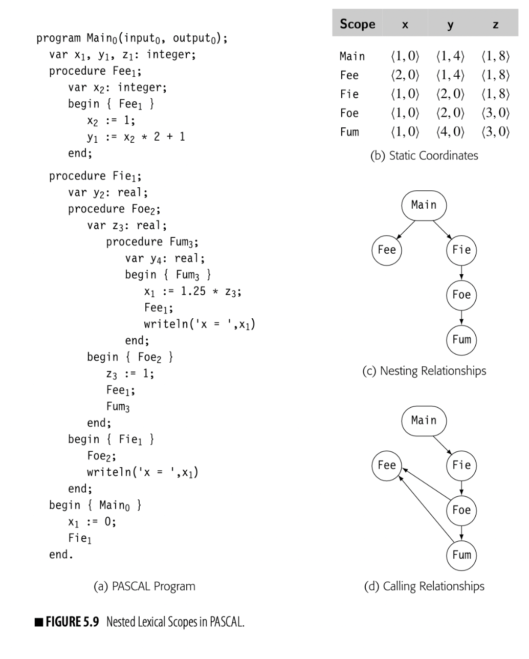
Modeling Lexical Scopes

As the parser works its way through the input code, it must build and maintain a model of the naming environment. The model changes as the parser enters and leaves individual scopes. The compiler's symbol table instantiates that model.

The compiler can build a separate table for each scope, as shown in Fig. 5.10. Panel (a) shows an outer scope $J$ that contains two inner scopes. 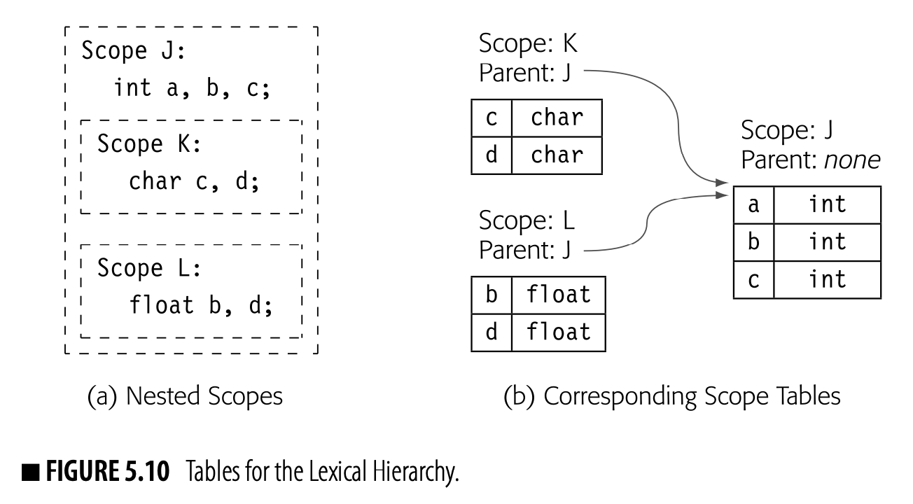In scope K, a and b have type int while c and d have type char. In scope L, a and c have type int while b and d have type float.

Scopes K and L are both nested inside scope J. Scopes K and L are otherwise unrelated.

Panel (b) shows the corresponding symbol tables. The table for a scope consists of both a hash table and a link to the surrounding scope. The gray arrows depict the search path, which reflects nesting in the code. Thus, a lookup of a in scope K would fail in the table for K, then follow the link to scope J, where it would find the definition of a as an int.

This approach lets the compiler create flexible, searchable models for the naming environment in each scope. A search path is just a list or chain of tables that specifies the order in which the tables will be searched. At compile time, a lookup for name resolution begins with the search path for the current scope and proceeds up the chain of surrounding scopes. Because the relationship between scopes is static (unchanging), the compiler can build scope-specific search paths with syntax-driven translation and preserve those tables and paths for use in later stages of the compiler and, if needed, in other tools.

Building the Model

The compiler writer can arrange to build the name-space model during syntax-driven translation. The source language constructs that enter and leave distinct scopes can trigger actions to create tables and search paths. The productions for declarations and references can create and refine the entries for names.

Block Democations such as begin and end, $\underline{{} an d \underline{}}$ , and procedure entry and exit, create a new table on entry to the scope and link it to the start of the search path for the block(s) associated with the current scope. On exit, the action should mark the table as final.

DYNAMIC SCOPING

The alternative to lexical scoping is dynamic scoping. The distinction between lexical and dynamic scoping only matters when a procedure refers to a variable that is declared outside the procedure’s own scope, sometimes called a free variable.

With lexical scoping, the rule is simple and consistent: a free variable is bound to the declaration for its name that is lexically closest to the use. If the compiler starts in the scope containing the use, and checks successive surrounding scopes, the variable is bound to the first declaration that it finds. The declaration always comes from a scope that encloses the reference.

With dynamic scoping, the rule is equally simple: a free variable is bound to the variable by that name that was most recently created at runtime. Thus, when execution encounters a free variable, it binds that free variable to the most recent instance of that name. Early implementations created a runtime stack of names on which every name was pushed as its defining occurrence was encountered. To bind a free variable, the running code searched the name stack from its top downward until a variable with the right name was found. Later implementations are more efficient.

While many early Lisp systems used dynamic scoping, lexical scoping has become the dominant choice. Dynamic scoping is easy to implement in an interpreter and somewhat harder to implement efficiently in a compiler. It can create bugs that are difficult to detect and hard to understand. Dynamic scoping still appears in some languages; for example, Common Lisp still allows the program to specify dynamic scoping.

Variable Declarations, if they exist, create entries for the declared names in the local table and populate them with the declared attributes. If they do not exist, then attributes such as type must be inferred from references. Some size information might be inferred from points where aggregates are allocated.
References trigger a lookup along the search path for the current scope. In a language with declarations, failure to find a name in the local table causes a search through the entire search path. In a language without declarations, the reference may create a local entity with that name; it may refer to a name in a surrounding scope. The rules on implicit decla- rations are language specific. FORTRAN creates the name with default attributes based on the first letter of the name. C looks for it in surrounding scopes and declares an error if it is not found. PYTHON’s actions depend on whether the first occurrence of the name in a scope is a definition or a use.

Examples

Lexical scope rules are generally similar across different programming languages. However, language designers manage to insert surprising and idiosyncratic touches. The compiler writer must adapt the general translation schemes described here to the specific rules of the source language.

C has a simple, lexically scoped name space. Procedure names and global variables exist in the global scope. Each procedure creates its own local scope for variables, parameters, and labels. C does not include nested procedures or functions, although some compilers, such as GCC, implement this extension. Blocks, set off by $\underline{{} an d \underline{}}$ , create their own local scopes; blocks can be nested.

The C keyword static both restricts a name's visibility and specifies its lifetime. A static global name is only visible inside the file that contains its declaration. A static local name has local visibility. Any static name has a global lifetime; that is, it retains its value across distinct invocations of the declaring procedure.

SCHEME has scope rules that are similar to those in C. Almost all entities in SCHEME reside in a single global scope. Entities can be data; they can be executable expressions. System-provided functions, such as cons, live alongside user-written code and data items. Code, which consists of an executable expression, can create private objects by using a let expression. Nesting 1et expressions inside one another can create nested lexical scopes of arbitrary depth.

PYTHON is an Algol-like language that eschews declarations. It supports three kinds of scopes: a local function-specific scope for names defined in a function; a global scope for names defined outside of any programmer-supplied function; and a builtin scope for implementation-provided names such as print. These scopes nest in that order: local embeds in global which embeds in builtin. Functions themselves can nest, creating a hierarchy of local scopes.

PYTHON does not provide type declarations. The first use of a name $x$ in a scope is its defining occurrence. If the first use assigns $x$ a value, then it binds $x$ to a new local entity with its type defined by the assigned value. If the first use refers to $x$ 's value, then it binds $x$ to a global entity; if no such entity exists, then that defining use creates the entity. If the programmer intends $x$ to be global but needs to define it before using it, the programmer can add a nonlocal declaration for the name, which ensures that $x$ is in the global scope.

TERMINOLOGY FOR OBJECT-ORIENTED LANGUAGES

The diversity of object-oriented languages has led to some ambiguity in the terms that we use to discuss them. To make the discussion in this chapter concrete, we will use the following terms: Object An object is an abstraction with one or more members. Those members can be data items, code that manipulates those data items, or other objects. An object with code members is a class. Each object has internal state-data whose lifetimes match the object's lifetime. Class A class is a collection of objects that all have the same abstract structure and characteristics. A class defines the set of data members in each instance of the class and defines the code members, or methods, that are local to that class. Some methods are public, or externally visible, while others are private, or invisible outside the class. Inheritance Inheritance is a relationship among classes that defines a partial order on the name scopes of classes. A class a may inherit members from its superclass. If a is the superclass of b, b is a subclass of a. A name x defined in a subclass obscures any definitions of x in a superclass. Some languages allow a class to inherit from multiple superclasses. Receiver Methods are invoked relative to some object, called the method's receiver. The receiver is known by a designated name inside the method, such as this or self.

The power of an $OOL$ arises, in large part, from the organizational possibilities presented by its multiple name spaces.

5.4.2 Inheritance Hierarchies

Object-oriented languages (OOLs) introduce a second form of nested name space through inheritance. OOLs introduce classes. A class consists of a collection (possibly empty) of objects that have the same structure and behavior. The class definition specifies the code and data members of an object in the class.

Polymorphism The ability of an entity to take on different types is often called polymorphism.

Much of the power of an OOL derives from the ability to create new classes by drawing on definitions of other existing classes. In JAVA terminology, a new class $β$ can extend an existing class $α$ ; objects of class $β$ then inherit definitions of code and data members from the definition of $α$ . $β$ may redefine names from $α$ with new meanings and types; the new definitions obscure earlier definitions in $α$ or its superclasses. Other languages provide similar functionality with a different vocabulary.

The terminology used to specify inheritance varies across languages. In JAVA, a subclass extends its superclass. In C++, a subclass is derived from its superclass.

Subtype polymorphism the ability of a subclass object to reference superclass members

Class extension creates an inheritance hierarchy: if $α$ is the superclass of $β$ , then any method defined in $α$ must operate correctly on an object of class $β$ , provided that the method is visible in $β$ . The converse is not true. A subclass method may rely on subclass members that are not defined in instances of the superclass; such a method cannot operate correctly on an object that is an instance of the superclass.

In a single-inheritance language, such as JAVA, inheritance imposes a tree-structured hierarchy on the set of classes. Other languages allow a class $β$ to have multiple immediate superclasses. This notion of "multiple inheritance" gives the programmer an ability to reuse more code, but it creates a more complex name resolution environment.

Each class definition creates a new scope. Names of code and data members are specific to the class definition. Many languages provide an explicit mechanism to control the visibility of member names. In some languages, class definitions can contain other classes to create an internal lexical hierarchy. Inheritance defines a second search path based on the superclass relationship.

In translation, the compiler must map an $⟨ o bj ec t, m e mb er ⟩$ pair back to a specific member declaration in a specific class definition. That binding provides the compiler with the type information and access method that it needs to translate the reference. The compiler finds the object name in the lexical hierarchy; that entry provides a class that serves as the starting point for the compiler to search for the member name in the inheritance hierarchy.

Modeling Inheritance Hierarchies

The lexical hierarchy reflects nesting in the syntax. The inheritance hierarchy is created by definitions, not syntactic position.

To resolve member names, the compiler needs a model of the inheritance hierarchy as defined by the set of class declarations. The compiler can build a distinct table for the scope associated with each class as it parses that class' declaration. Source-language phrases that establish inheritance cause the compiler to link class scopes together to form the hierarchy. In a single-inheritance language, the hierarchy has a tree structure; classes are children of their superclasses. In a multiple-inheritance language, the hierarchy forms an acyclic graph.

The compiler uses the same tools to model the inheritance hierarchy that it does to model the lexical hierarchy. It creates tables to model each scope. It links those tables together to create search paths. The order in which those searches occur depends on language-specific scope and inheritance rules. The underlying technology used to create and maintain the model does not.

Compile-Time Versus Runtime Resolution

Closed class structure If the class structure of an application is fixed at compile time, the OOL has a closed hierarchy.

The major complication that arises with some OOLs derives not from the presence of an inheritance hierarchy, but rather from when that hierarchy is defined. If the OOL requires that class definitions be present at compile time and that those definitions cannot change, then the compiler can resolve member names, perform appropriate type checking, determine appropriate access methods, and generate code for member-name references. We say that such a language has a closed class structure.

By contrast, if the language allows the running program to change its class structure, either by importing class definitions at runtime, as in JAVA, or by editing class definitions, as in SMALLtalk, then the language may need to defer some name resolution and binding to runtime. We say that such a language has an open class structure.

Lookup with Inheritance

Assume, for the moment, a closed class structure. Consider two distinct scenarios:

Qualified name a multipart name, such asx.part, where part is an element of an aggregate entity named x

If the compiler finds a reference to an unqualified name $n$ in some procedure $p$ , it searches the lexical hierarchy for $n$ . If $p$ is a method defined in some class $c$ , then $n$ might also be a data member of $c$ or some superclass of $c$ ; thus, the compiler must insert part of the inheritance hierarchy into the appropriate point in the search path.
If the compiler finds a reference to member $m$ of object $o$ , it first resolves $o$ in the lexical hierarchy to an instance of some class $c$ . Next, it searches for $m$ in the table for class $c$ ; if that search fails, it looks for $m$ in each table along $c$ 's chain of superclasses (in order). It either finds $m$ or exhausts the hierarchy.

One of the primary sources of opportunity for just-in-time compilers is lowering the costs associated with runtime name resolution.

With an open class structure, the compiler may need to generate code that causes some of this name resolution to occur at runtime, as occurs with a virtual function in C++. In general, runtime name resolution replaces a simple, often inexpensive, reference with a call to a more expensive runtime support routine that resolves the name and provides the appropriate access (read, write, or execute).

Building the Model

As the parser processes a class definition, it can (1) enter the class name into the current lexical scope and (2) create a new table for the names defined in the class. Since both the contents of the class and its inheritance context are specified with syntax, the compiler writer can use syntax-drivenactions to build and populate the table and to link it into the surrounding inheritance hierarchy. Member names are found in the inheritance hierarchy; unqualified names are found in the lexical hierarchy. 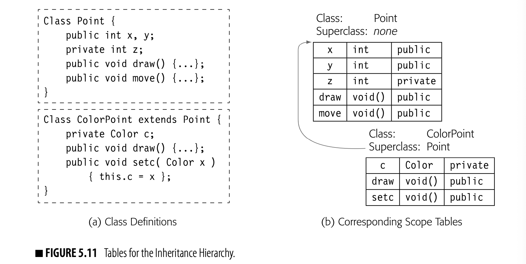The compiler can use the symbol-table building blocks designed for lexical hierarchies to represent inheritance hierarchies. Fig. 5.11 shows two class definitions, one for Point and another for ColorPoint, which is a subclass of Point. The compiler can link these tables into a search path for the inheritance hierarchy, shown in the figure as a SuperClass pointer. More complicated situations, such as lexically nested class definitions, simply produce more complex search paths.

Examples

Object-oriented languages differ in the vocabulary that they use and in the object-models that they use.

C++ has a closed class structure. By design, method names can be bound to implementations at compile time. C++ includes an explicit declaration to force runtime binding--the C++ virtual function.

By contrast, JAVA has an open class structure, although the cost of changing the class structure is high--the code must invoke the class loader to import new class definitions. A compiler could, in principle, resolve method names to implementations at startup and rebind after each invocation of the class loader. In practice, most JAVA systems interpret bytecode and compile frequently executed methods with a just-in-time compiler. This approach allows high-quality code and late binding. If the class loader overwrites some class definition that was used in an earlier JIT-compilation, it can force recompilation by invalidating the code for affected methods.

Multiple Inheritance

Multiple inheritance a feature that allows a class to inherit from multiple immediate superclasses

Some OOLs allow multiple inheritance. The language needs syntax that lets a programmer specify that members $a$ , $b$ , and $c$ inherit their definitions from superclass $x$ while members $d$ and $e$ inherit their definitions from superclass $y$ . The language must resolve or prohibit nonsensical situations, such as a class that inherits multiple definitions of the same name.

To support multiple inheritance, the compiler needs a more complex model of the inheritance hierarchy. It can, however, build an appropriate model from the same building blocks: symbol tables and explicit search paths. The complexity largely manifests itself in the search paths.

5.4.3 Visibility

Visibility A name is visible at point p if it can be referenced at p. Some languages provide ways to control a name’s visibility.

Programming languages often provide explicit control over visibility--that is, where in the code a name can be defined or used. For example, C provides limited visibility control with the static keyword. Visibility control arises in both lexical and inheritance hierarchies.

C's static keyword specifies both lifetime and visibility. A C static variable has a lifetime of the entire execution and its visibility is restricted to the current scope and any scopes nested inside the current scope. With a declaration outside of any procedure, static limits visibility to code within that file. (Without static, such a name would be visible throughout the program.)

For a C static variable declared inside a procedure, the lifetime attribute of static ensures that its value is preserved across invocations. The visibility attribute of static has no effect, since the variable's visibility was already limited to the declaring procedure and any scopes nested inside it.

JAVA provides explicit control over visibility via the keywords public, private, protected, and default.

public A public method or data member is visible from anywhere in the program.
private A private method or data member is only visible within the class that encloses it.
protected A protected method or data member is visible within the class that encloses it, in any other class declared in the same package, and in any subclass declared in a different package.
default A default method or data member is visible within the class that encloses it and in any other class declared in the same package. If no visibility is specified, the object has default visibility.

Neither private nor protected can be used on a declaration at the top level of the hierarchy because they define visibility with respect to the enclosing class; at the top level, a declaration has no enclosing class.

As the compiler builds the naming environment, it must encode the visibility attributes into the name-space model. A typical implementation will include a visibility tag in the symbol table record of each name. Those tags are consulted in symbol table lookups.

As mentioned before, PYTHON determines a variable's visibility based on whether its defining occurrence is a definition or a use. (A use implies that the name is global.) For objects, PYTHON provides no mechanism to control visibility of their data and code members. All attributes (data members) and methods have global visibility.

5.4.4 Performing Compile-Time Name Resolution

During translation, the compiler often maps a name's lexeme to a specific entity, such as a variable, object, or procedure. To resolve a name's identity, the compiler uses the symbol tables that it has built to represent the lexical and inheritance hierarchies. Language rules specify a search path through these tables. The compiler starts at the innermost level of the search path. It performs a lookup on each table in the path until it either finds the name or fails in the outermost table.

The specifics of the path are language dependent. If the syntax of the name indicates that it is an object-relative reference, then the compiler can start with the table for the object's class and work its way up the inheritance hierarchy. If the syntax of the name indicates that it is an "ordinary" program variable, then the compiler can start with the table for the scope in which the reference appears and work its way up the lexical hierarchy. If the language's syntax fails to distinguish between data members of objects and ordinary variables, then the compiler must build some hybrid search path that combines tables in a way that models the language-specified scope rules.

The compiler can maintain the necessary search paths with syntax-driven actions that execute as the parser enters and leaves scopes, and as it enters and leaves declarations of classes, structures, and other aggregates. The details, of course, will depend heavily on the specific rules in the source language being compiled.

SECTION REVIEW

Programming languages provide mechanisms to control the lifetime and visibility of a name. Declarations allow explicit specification of a name’s properties. The placement of a declaration in the code has a direct effect on lifetime and visibility, as defined by the language’s scope rules. In an object-oriented language, the inheritance environment also affects the properties of a named entity.

To model these complex naming environments, compilers use two fundamental tools: symbol tables and search paths that link tables together in a hierarchical fashion. The compiler can use these tools to construct context-specific search spaces that model the source-language rules.

REVIEW QUESTIONS

Assume that the compiler builds a distinct symbol table and search path for each scope. For a simple PASCAL-like language, what actions should the parser take on entry to and exit from each scope?
Using the table and search path model for name resolution, what is the asymptotic cost of (a) resolving a local name? (b) resolving a nonlocal name? (Assume that table lookup has a $O (1)$ cost.) In programs that you have written, how deeply have you nested scopes?

5.5 Type Information

Type an abstract category that specifies properties held in common by all members of the type Common types include integer, character, list, and function.

In order to translate references into access methods, the compiler must know what the name represents. A source language name fee might be a small integer; it might be a function of two character strings that returns a floating-point number; it might be an object of class fum. Before the front end can emit code to manipulate fee, it must know fee's fundamental properties, summarized as its type.

A type is just a collection of properties; all members of the type have the same properties. For example, an integer might be defined as any whole number $i$ in the range $- 2^{63} \leq i < 2^{63} - 1$ , or red might be a value in the enumerated type colors defined as the set ${red, yellow, blue}$ .

We represent the type of a structure as the product of the types of its constituent fields, in order.

Types can be specified by rules; for example, the declaration of a structure in C defines a type. The structure's type specifies the set of declared fields and their order inside the structure; each field has its own type that specifies its interpretation. Programming languages predefine some types, called base_types. Most languages allow the programmer to construct new types. The set of types in a given language, along with the rules that use types to specify program behavior, are collectively called a type system.

The type system allows both language designers and programmers to specify program behavior at a more precise level than is possible with a context-free grammar. The type system creates a second vocabulary for describing the behavior of valid programs. Consider, for example, the JAVA expression a+b. The meaning of + depends on the types of a and b. If a and b are strings, the + operator specifies concatenation. If a and b are numbers, the + operator specifies addition, perhaps with implicit conversion to a common type. This kind of overloading requires accurate type information.

5.5.1 Uses for Types in Translation

Types play a critical role in translation because they help the compiler understand the meaning and, thus, the implementation of the source code. This knowledge, which is deeper than syntax, allows the compiler to detect errors that might otherwise arise at runtime. In many cases, it also lets the compiler generate more efficient code than would be possible without the type information.

Conformable We will say that an operator and its operands are conformable if the result of applying the operator to those arguments is well defined.

The compiler can use type information to ensure that operators and operands are conformable--that is, that the operator is well defined over the operands' types (e.g., string concatenation might not be defined over real numbers). In some cases, the language may require the compiler to insert code to convert nonconformable arguments to conformable types--a process called implicit conversion. In other cases (e.g., using a floating-point number as a pointer), the language definition may disallow such conversion; the compiler should, at a minimum, emit an informative error message to give the programmer insight into the problem.

If x is real but provably 2, there are less expensive ways to compute ax than with a Taylor series.

Type information can lead the compiler to translations that execute efficiently. For example, in the expression $a^{x}$ , the types of $a$ and $x$ determine how best to evaluate the expression. If $x$ is a nonnegative integer, the compiler can generate a series of multiplications to evaluate $a^{x}$ . If, instead, $x$ is a real number or a negative number, the compiler may need to generate code that uses a more complex evaluation scheme, such as a Taylor-series expansion. (The more complicated form might be implemented via a call to a support library.) Similarly, languages that allow whole structure or whole array assignment rely on conformability checking to let the compiler implement these constructs in an efficient way.

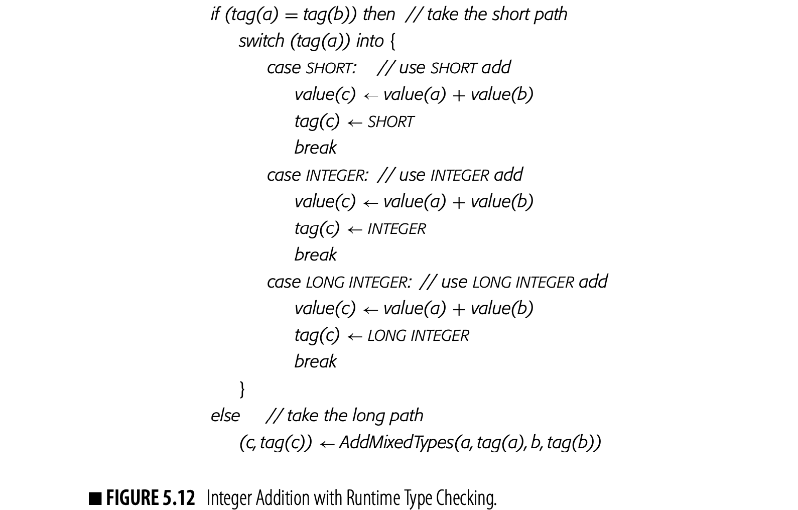
Type signature a specification of the types of the formal parameters and return value(s) of a function

Function prototype The C language includes a provision that lets the programmer declare functions that are not present. The programmer includes a skeleton declaration, called a function prototype.

At a larger scale, type information plays an important enabling role in modular programming and separate compilation. Modular programming creates the opportunity for a programmer to mis-specify the number and types of arguments to a function that is implemented in another file or module. If the language requires that the programmer provide a type signature for any externally defined function (essentially, a C function prototype), then the compiler can check the actual arguments against the type signature.

Type information also plays a key role in garbage collection (see Section 6.6.2). It allows the runtime collector to understand the size of each entity on the heap and to understand which fields in the object are pointers to other, possibly heap-allocated, entities. Without type information, collected at compile time and preserved for the collector, the collector would need to conservatively assume that any field might be a pointer and apply runtime range and alignment tests to exclude out-of-bounds values.

Lack of Type Information

Complete type information might be un- available due to language design or due to late binding.

If type information is not available during translation, the compiler may need to emit code that performs type checking and code selection at runtime. Each entity of unknown type would need a runtime tag to hold its type. Instead of emitting a simple operator, the compiler would need to generate case logic based on the operand types, both to perform tag generation and to manipulate the values and tags.

Fig. 5.12 uses pseudocode to show what the compiler might generate for addition with runtime checking and conversion. It assumes three types, SHORT, INTEGER, and LONG INTEGER. If the operands have the same type, the code selects the appropriate version of the addition operator, performs the arithmetic, and sets the tag. If the operands have distinct types, it invokes a library routine that performs the complete case analysis, converts operands appropriately, adds the converted operands, and returns the result and its tag.

By contrast, of course, if the compiler had complete and accurate type information, it could generate code to perform both the operation and any necessary conversions directly. In that situation, runtime tags and the associated tag-checking would be unnecessary.

5.5.2 Components of a Type System

A type system has four major components: a set of base types, or built-in types; rules to build new types from existing types; a method to determine if two types are equivalent; and rules to infer the type of a source-language expression.

Base Types

The size of a “word” may vary across im- plementations and processors.

Most languages include base types for some, if not all, of the following kinds of data: numbers, characters, and booleans. Most processors provide direct support for these kinds of data, as well. Numbers typically come in several formats, such as integer and floating point, and multiple sizes, such as byte, word, double word, and quadruple word.

Individual languages add other base types. LISP includes both a rational number type and a recursive-list type. Rational numbers are, essentially, pairs of integers interpreted as a ratio. A list is either the designated value nil or a list built with the constructor cons; the expression (cons first rest) is an ordered list where first is an object and rest is a list.

Languages differ in their base types and the operators defined over those base types. For example, C and C++ have many varieties of integers; long int and unsigned long int have the same length, but support different ranges of integers. PYTHON has multiple string classes that provide a broad set of operations; by contrast, C has no string type so programmers use arrays of characters instead. C provides a pointer type to hold an arbitrary memory address; JAVA provides a more restrictive model of reference types.

Compound and Constructed Types

Some languages provide higher-level abstractions as base types, such as PYTHON maps.

The base types of a programming language provide an abstraction for the actual kinds of data supported by the processor. However, the base types are often inadequate to represent the information domain that the programmer needs--abstractions such as graphs, trees, tables, records, objects, classes, lists, stacks, and maps. These higher-level abstractions can be implemented as collections of multiple entities, each with its own type.

In an OOL, classes can be treated as con- structed types. Inheritance defines a subtype relationship, or specialization.

The ability to construct new types to represent compound or aggregate objects is an essential feature of many languages. Typical constructed types include arrays, strings, enumerated types, and structures or records. Compound types let the programmer organize information in novel, program-specific ways. Constructed types allow the language to express higher-level operations, such as whole-structure assignment. They also improve the compiler's ability to detect ill-formed programs.

Arrays

Arrays are among the most widely used aggregate objects. An array groups together multiple objects of the same type and gives each a distinct name--albeit an implicit, computed name rather than an explicit, programmer-designated name. The C declaration int a[100][200]; sets aside space for $100 \times 200 = 20$ ,000 integers and ensures that they can be addressed using the name a. The references a[1][17] and a[2][30] access distinct and independent memory locations. The essential property of an array is that the program can compute names for each of its elements by using numbers (or some other ordered, discrete type) as subscripts.

Array conformability Two arrays a and b are conformable with respect to some array operator if the di- mensions of a and b make sense with the operator. Matrix multiply, for example, imposes different conformability requirements than does matrix addition.

Support for operations on arrays varies widely. FORTRAN 90, PL/I, and apl all support assignment of whole or partial arrays. These languages support element-by-element application of arithmetic operations to arrays. For conformable arrays x, y, and z, the statement $x = y + z$ would overwrite each x[i,j] with y[i,j]+z[i,j]. Apl takes the notion of array operations further than most languages; it includes operators for inner product, outer product, and several kinds of reductions. For example, the sum reduction of y, written $x \leftarrow + / y$ , assigns x the scalar sum of the elements of y.

An array can be viewed as a constructed type because it is specified with the type of its elements. Thus, a 10 x 10 array of integers has type two-dimensional array of integers. Some languages include the array's dimensions in its type; thus, a 10 x 10 array of integers has a different type than a 12 x 12 array of integers. This approach makes array operations where the operands have incompatible dimensions into type errors; thus, they are detected and reported in a systematic way. Most languages allow arrays ofany base type; some languages allow arrays of constructed types, such as structures, as well.

Strings

Support for strings varies across languages. Some languages, such as PYTHON or PL/I, support multiple kinds of strings with similar properties, attributes, and operations. Others, such as FORTRAN or C, simply treat a string as a vector of characters.

A true string type differs from an array type in several important ways. Operations that make sense on strings, such as concatenation, translation, and computing string length, may not have analogs for arrays. The standard comparison operators can be overloaded so that string comparisons work in the natural way: "a" < "boo" and "fee" < "fie". Implementing a similar comparison for arrays of characters suggests application of the idea to arrays of numbers or structures, where the analogy may not hold. Similarly, the actual length of a string may differ from its allocated size, while most applications of an array use all the allocated elements.

Enumerated Types

Many languages let the programmer construct a type that contains a specific set of constant values. An enumerated type lets the programmer use self-documenting names for small sets of constants. Classic examples include the days of the week and the months of the year. In C syntax, these might be written

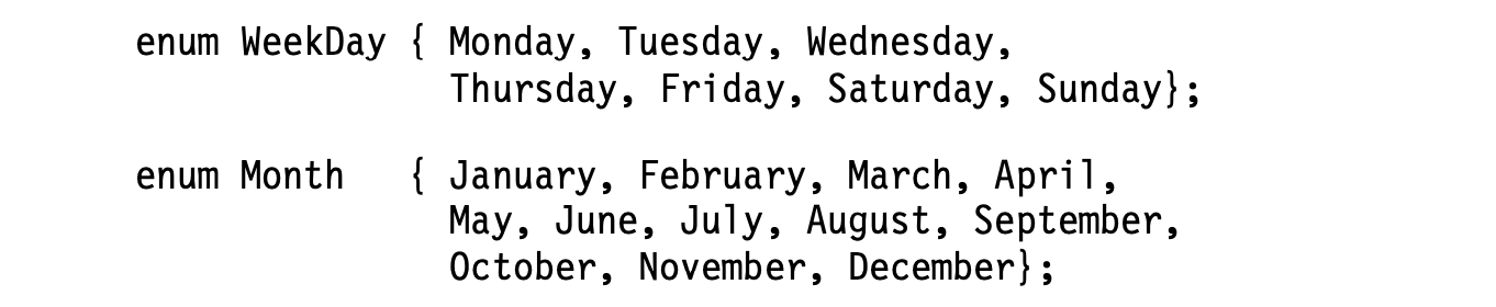
The compiler maps each element of an enumerated type to a distinct value. The elements of an enumerated type are ordered, so comparisons between elements of the same type make sense. In the examples, $M o n d a y < T u es d a y$ and $J u n e < J u l y$ . Operations that compare different enumerated types make no sense--for example, $T u es d a y > S e pt e mb er$ should produce a type error. PASCAL ensures that each enumerated type behaves as if it were a subrange of the integers. For example, the programmer can declare an array indexed by the elements of an enumerated type.

Structures and Variants

Structures, or records, group together multiple objects of arbitrary type. The elements of the structure are typically given explicit names. For example, a programmer implementing a parse tree in C might need nodes with both one and two children.

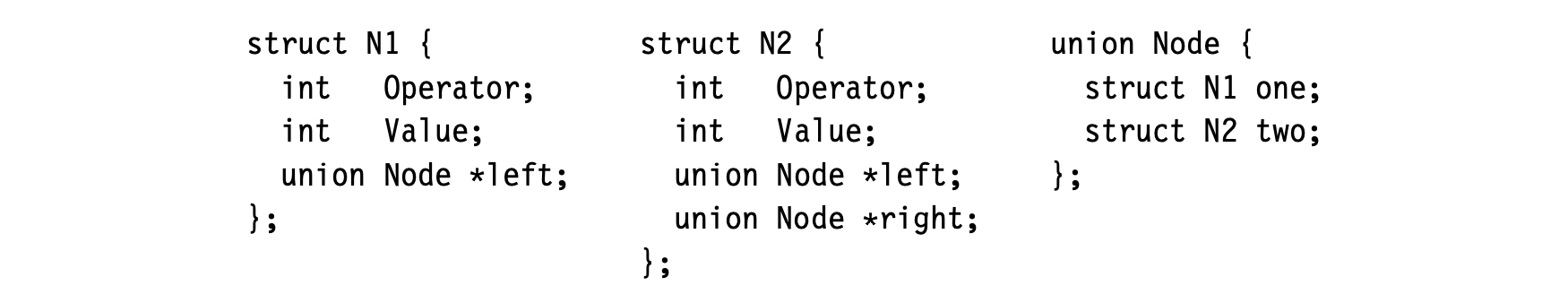
The type of a structure is the ordered product of the types of the elements that it contains. We might describe N1 and N2 as:

These new types should have the same essential properties that a base type has. In C, autoincrementing a pointer to an N1 or casting a pointer into an (N1 *) has the desired effect--the behavior is analogous to what happens for a base type.

The example creates a new type, Node, that is a structure of either type N1 or type N2. Thus, the pointer in an N1 node can reference either an N1 node or an N2 node. PASCAL creates unions with variant records. C uses a union. The type of a union is the alternation of its component types; thus, Node has type $N 1 \cup N 2$ .

Between them, the language and the runtime need a mechanism to disambiguate references. One solution is fully qualified references as in p $\to$ Node.N1.Value versus p $\to$ Node.N2.Value. Alternatively, the language might adopt PASCAL's strategy and require runtime tags for variant records, with explicit checks for the tags at runtime.

Objects and Classes

In an object-oriented language, classes define both the content and form of objects, and they define the inheritance hierarchy that is used to resolve object-relative references. In implementation, however, an object looks like a record or structure whose organization is specified by the class definition.

An alternative view of structures

The classical view of structures treats each kind of structure as a distinct type. This approach to structure types follows the treatment of other aggregates, such as arrays and strings. It seems natural. It makes distinctions that are useful to the programmer. For example, a tree node with two children probably should have a different type than a tree node with three children; presumably, they are used in different situations. A program that assigns a three-child node to a two-child node should generate a type error and a warning message to the programmer.

From the runtime system's perspective, however, treating each structure as a distinct type complicates matters. With distinct structure types, the heap contains a set of objects drawn from an arbitrary set of types. This makes it difficult to reason about programs that deal directly with the objects on the heap, such as a garbage collector. To simplify such programs, their authors sometimes take a different approach to structure types.

This alternate model considers all structures in the program as a single type. Individual structure declarations each create a variant form of the type structure. The type structure, itself, is the union of all these variants. This approach lets the program view the heap as a collection of objects of a single type, rather than a collection of many types. This view makes code that manipulates the heap simpler to analyze and optimize.

Type Equivalence

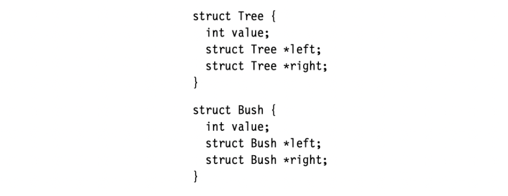The compiler needs a mechanism to determine if two constructed types are equivalent. (The answer is obvious for base types.) Consider the C structure declarations shown in the margin. Are Tree and Bush the same type? Are they equivalent? Any language that includes constructed types needs an unambiguous rule to answer this question. Historically, languages have taken one of two approaches.

Name Equivalence asserts that two types are equivalent if and only if the programmer calls them by the same name. This approach assumes that naming is an intentional act and that the programmer uses names to impart meaning.
Structural Equivalence asserts that two types are equivalent if and only if they have the same structure. This approach assumes that structure matters and that names may not.

Tree and Bush have structural equivalence but not name equivalence.

Each approach has its adherents and its detractors. However, the choice between them is made by the language designer, not the compiler writer. Thecompiler writer must implement an appropriate representation for the type and an appropriate equivalence test.

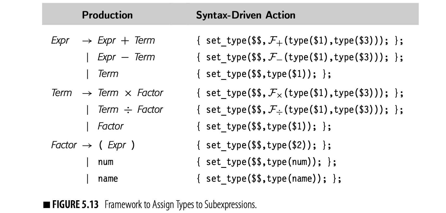
5.5.3 Type Inference for Expressions

The compiler must assign, to each expression and subexpression, a specific type. The simplest expressions, names and nums, have well defined types. For expressions computed from references, the compiler must infer the type from the combination of the operation and the types of its operands.

The relationship between operator, operand types, and result type must be specified for the compiler to infer expression types. Conceptually, we can think of the relationship as a recursive function over the tree; in practice, the rules vary from simple and obvious to arcane. The digression on page 248 describes the rules for expressions in C++. Because C++ has so many base types, its rules are voluminous.

The result type of an expression depends on the operator and the types of its operands. The compiler could assign types in a bottom-up walk over an expression tree. At each node, it would set the node's type from the type of its operator and its children. Alternatively, the compiler could assign types as part of its syntax-driven framework for translation.

Fig. 5.13 sketches the actions necessary to assign types to subexpressions in a syntax-driven framework. It assumes that the type-function for an operator $α$ is given by a function $F_{α}$ . Thus, the type of a multiplication is just $F_{\times} (t_{1}, t_{2})$ , where $t_{1}$ and $t_{2}$ are the types of the left and right operands of $\times$ . Of course, the compiler writer would likely pass a structured value on the stack, so the references to $5, $1, and $3 would be more complex.

NUMERICAL CONVERSIONS IN C++

C++, as defined in the ISO 2017 standard, has a large and complex set of conversion rules [212]. Here is a simplified version of the promotion and conversion rules for numerical values.

Integral Promotion: A character value or a value in an untyped enumeration can be promoted to the first integer type that will hold all of its values. The integer types, in order, are: int, unsigned int, long int, unsigned long int, long long int, and unsigned long long int. (For a typed enumeration, conversion is legal only if the underlying type converts to integer.)

Floating-Point Promotion: A float value can be promoted to type double.

Integer Conversions: A value of an integer type can be converted to another integer type, as can a value of an enumeration type. For an unsigned destination type, the result is the smallest unsigned integer congruent to the source value. For a signed destination type, the value is unchanged if it fits in the destination type, otherwise the result is implementation-defined.

Floating-Point Conversions: A value of floating-point type can be converted to another floating-point type. If the destination type can exactly represent the source value, the result is that value. Otherwise it is an implementation-defined choice between the two adjacent values.

Boolean Conversion: A numerical value, enumeration value, or pointer value can be converted to a value of type bool. A value of zero, a null pointer, or a null member pointer all convert to false; any other value converts to true.

The compiler tries to convert the source value to the destination type, which may involve both a promotion and a conversion.

In a language with more complex inference rules, the compiler might build an IR that has incomplete type information and perform one or more passes over the IR to assign types to subexpressions.

The Role of Declarations

Programming languages differ on whether or not they require declarations. In a language with mandatory declarations, the declarations establish a concrete type for every named entity; those types serve, in turn, as the initial information for type inference. In a language without declarations, such as python or LISP, the compiler must infer types for values from the context in which they appear in the code. For example, the assignment fee - 'a'might imply that $fee$ has a type that can hold a single character, while $fee \leftarrow$ "a" implies that $fee$ can hold a character string.

Programming languages also differ on where in the code a declaration must appear. Many languages have a "declare before use" rule; any name must be declared before it appears in the executable code. This rule facilitates type-checking during the parser's translation into an initial IR form. Languages that do not require declaration before use force the compiler to build an initial IR that abstracts away details of type, and to subsequently perform type inference and checking on that abstract IR so that the compiler can refine operators and references to reflect the correct type information.

Mixed-Type Expressions

This example assumes the C convention of single quotes for characters and double quotes for strings.

Programming languages differ on the extent to which they expect the compiler to insert type conversions when the code specifies an expression with types that are not directly compatible. For example, an expression $a \times b$ may be defined for the case when $a$ and $b$ are both integers or both floating-point numbers, but not when $a$ is an integer and $b$ is a floating-point number. The language may require the compiler to report an error; alternatively, it might require the compiler to insert a conversion. Section 7.2.2 discusses the implementation of implicit conversions.

For example, ANSI C++ supports multiple kinds of integers that differ in the range of numbers that each can represent. The language definition requires that the compiler insert code to convert between these representations; the definition specifies the behavior with a set of rules. Its rules specify the conversions for the division of an integer by a floating-point number and forbid division by a character string.

Interprocedural Aspects of Type Inference

Type inference for expressions depends, inherently, on the other procedures that form the executable program. In even the simplest type systems, expressions contain function calls. The compiler must check each of those calls. It must ensure the type compatibility of each actual parameter with the corresponding formal parameter. It must determine the type of the returned value for use in further inference.

To analyze and understand procedure calls, the compiler needs a type signature for each function. For example, in C's standard library, $strlen$ computes a character string's length. Its function prototype is:

This prototype asserts that strlen takes an argument of type char *. The const attribute indicates that strlen does not modify s. It returns a nonnegative integer. The type signature might be written: which we read as "strlen is a function that takes a constant-valued character string and returns an unsigned integer."

As a second example, filter in SCHEME has the type signature:

filter returns a list that contains every element of the input list for which the input function returns true.

That is, filter is a function of two arguments. The first should be a function that maps some type $α$ into a boolean, written ( $α \to b oo l e an$ ), and the second should be a list whose elements are of the same type $α$ . Given arguments of those types, filter returns a list whose elements have type $α$ . The function filter exhibits parametric polymorphism: its result type is a function of its argument types.

To perform accurate type inference, the compiler needs a type signature for every function. It can obtain that information in several ways. The compiler can require that the entire program be present for compilation, eliminating separate compilation. The compiler can require a type signature for each function, typically done with mandatory function prototypes. The compiler can defer type checking until link time or runtime, when such information is available. Finally, the compiler writer can embed the compiler in a programming system that gathers the requisite information. Each of these approaches has been used in real systems.

Section Review

A type represents a set of properties common to all values of that type. A type system assigns a type to each value in a program. Programming languages use types to define legal and illegal behavior. A good type system can increase language expressiveness, expose subtle errors, and let the compiler avoid runtime type checks.

A type system consists of a set of base types, rules to construct new types from existing ones, a method to determine the equivalence of two types, and rules to infer the type of an expression. The notions of base types, constructed types, and type equivalence should be familiar from most high-level languages.

REVIEW QUESTIONS

For your favorite programming language, what are its base types? Is there a mechanism to build an aggregate type? Does it provide a mech- anism for creating a procedure that takes a variable number of argu- ments, such as printf in the C standard I/O library? Hint: It may require interaction with the linker or the runtime system.

Type safety at procedure calls is often based on the use of prototypes— a declaration of the procedure’s arguments and return values. Sketch a mechanism that could ensure the validity of those function prototypes.

5.6 Storage Layout

Given a model of the name space and type information for each named entity, the compiler can perform storage layout. The process has two steps. First, the compiler must assign each entity to a logical data area. This decision depends on both the entity's lifetime and its visibility. Second, for each logical data area, the compiler assigns each entity in that area an offset from the data area's start.

5.6.1 Storage Classes and Data Areas

The compiler can classify values that need storage by their lifetimes. Most programming languages let programmers create values in at least the following storage classes: automatic, static, and irregular. The compiler maps a specific variable name into a storage area based on its lifetime, storage class, and visibility (see Section 4.7.3).

Automatic Variables

An automatic variable $a$ has a lifetime that is identical to the lifetime of its declaring scope. Therefore, it can be stored in the scope's local data area. For example, if $a$ is declared in procedure $p$ , the compiler can store $a$ in $p$ 's local data area. (If the scope is contained in $p$ , the compiler can set aside space for the scope inside $p$ 's local data area.) If $a$ is local, scalar, and unambiguous, the compiler may choose to store it in a register (see Section 4.7.2).

Activation record a region of memory set aside to hold con- trol information and the local data area for an invocation of a procedure We treat “activation” and “invocation” as synonyms.

To manage the execution of procedure $p$ , the compiler must ensure that each invocation of $p$ has a small block of storage to hold the control information needed by the call and return process. This activation record (AR) will also contain the arguments passed to $p$ as parameters. ARs are, in principle and in practice, created when control enters a procedure and freed when control exits that procedure.

Activation record pointer At runtime, the code will maintain a pointer to the current AR. The activation record pointer (ARP) almost always resides in a register for quick access.

The compiler can place $p$ 's local data area inside its ar. Each call to $p$ will create a new ar and, with it, a new local data area. This arrangement ensures that the local data area's lifetime matches the invocation's lifetime. It handles recursive calls correctly; it creates a new local data area for each call. Placing the local data area in the ar provides efficient access to local variables through the activation record pointer (arp). In most implementations, the local data area occupies one end of the procedure's ar (see Section 6.3.1).

Static Variables

A static variable $s$ has a lifetime that runs from the first time the executing program defines $s$ through the last time that the execution uses $s$ 's value. The first definition and last use of $s$ could cover a short period in the execution; they could also span the entire execution. The attribute static is typically implemented to run from the start of execution to its end.

Programming languages support static variables with a variety of visibility constraints. A global variable is static; it has visibility that spans multiple, nonnested procedures. A static variable declared inside a procedure has procedure-wide visibility (including nested scopes); the variable retains its value across multiple invocations of the procedure, much like a global variable. C uses static to create a file-level visibility; the value is live for the entire execution but only visible to procedures defined inside the same file.

Compilers create distinct data areas for static variables. In principle, a program could implement individual data areas for each static variable; alternatively, it could lump them all together into a single area. The compiler writer must develop a rationale that determines how static variables map into individual data areas. A simple approach is to create a single static data area per file of code and rely on the compiler's name resolution mechanism to enforce visibility constraints.

Compilers typically use assembly language constructs to create and initialize static data areas, so allocation, initialization, and deallocation have, essentially, no runtime cost. The compiler must create global data areas in a way that allows the system's linker to map all references to a given global name to the same storage location--the meaning of "global" visibility.

Irregular Entities

If a heap-allocated value has exactly one allocation, either the programmer or the compiler can convert it to a static lifetime.

Some values have lifetimes that are under program control, in the sense that the code explicitly allocates space for them. (Deallocation may be implicit or explicit.) The key distinction is that allocation and deallocation occur at times unrelated to any particular procedure's lifetime and have the potential to occur multiple times in a single execution.

Heap a region of memory set aside for irregu- lar entities and managed by the runtime support library

The compiler's runtime support library must provide a mechanism to allocate and free these irregular entities. Systems commonly use a runtime heap for such purposes. Control of the heap may be explicit, through calls such as LINUX's malloc and free. Alternatively, the heap may be managed with implicit deallocation through techniques such as garbage collection or reference counting.

While storage for the actual entities may be on the heap, the source code typically requires a name to begin a reference or chain of references. Thus, a linked list might consist of an automatic local variable, such as root, that contains a pointer to the first element of the list. root would need space in a register or the local data area, while the individual list elements might be allocated on the heap.

Temporary Values

Optimization can extend a temporary value’s lifetime. If the code recomputes $b \times c$ , the compiler might preserve its value rather than compute it twice (see Section 8.4.1).

During execution, a program computes many values that are never stored into named locations. For example, when compiled code evaluates $a - b \times c$ , it computes the value of $b \times c$ but has no semantic reason to retain its value. Because these temporary values have no names, they cannot be reused by the programmer. They have brief lifetimes.

When a temporary value has a representation that can fit in a register, the compiler should try to keep that value in a register. Some temporary values cannot fit in a register. Others have unknown lengths. For example, if d and e are strings of unknown length and $+$ is concatenation, then one scheme to evaluate $l e n g t h (d + e)$ creates the string temporary $d + e$ , also of unknown length.

The compiler can place large values of known or bounded length at the end of the local data area. If the length cannot be bounded, the compiler may need to generate code that performs a runtime allocation to create space for the value on the heap.

5.6.2 Layout Within a Virtual Address Space

Virtual address space In many systems, each process has an ad- dress space that is isolated from those of other processes. These address spaces are virtual, in the sense that they are not tied directly to physical memory (see Fig. 5.15).

The compiler must plan how the code will use memory at runtime. In most systems, each program runs in a distinct virtual address space; the program executes in its own protected range of addresses. The operating system and the underlying hardware map that virtual address space onto the actual physical hardware in a transparent fashion; the compiler only concerns itself with virtual addresses. 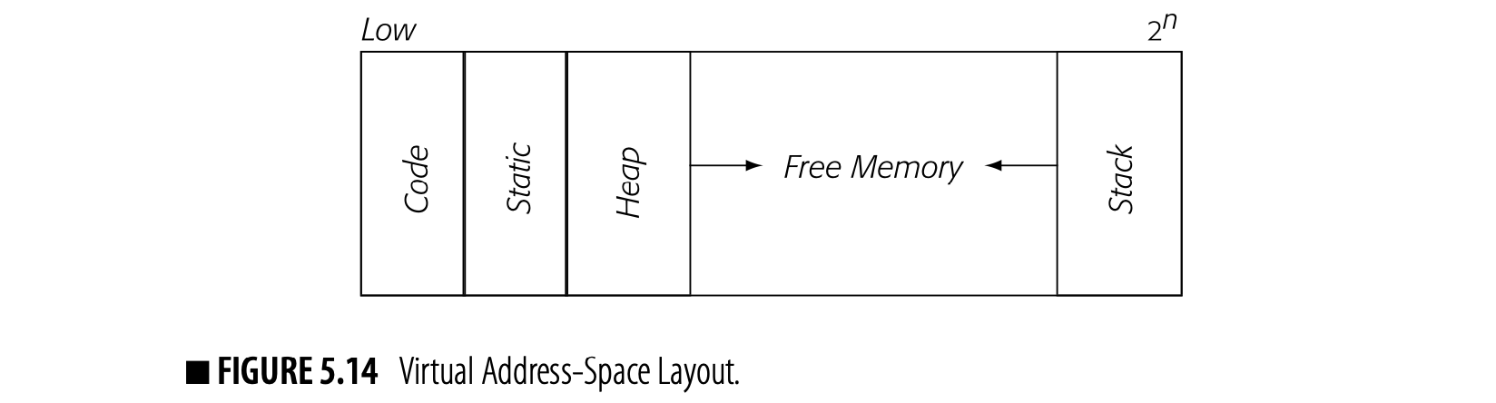The layout of the virtual address space is determined by an agreement among the operating system, hardware, and compiler. While minor details differ across implementations, most systems resemble the layout shown Fig. 5.14. The address space divides into four categories of storage:

Code: At one end of the address space, the compiler places executable code. Compiled code has, in general, known size. It rarely changes at runtime. If it changes size at runtime, the new code generally lives in a heap-allocated block of storage. Static: The second category of storage holds statically defined entities. This category includes global and static variables. The size of the static area can be determined at link time, when all of the code and data is combined to form an executable image.

In some circumstances, activation records must be heap allocated (see Section 6.3.1).

Heap: The heap is a variable-sized region of memory allocated under explicit program control. Dynamically allocated entities, such as variable-sized data structures or objects (in an OOL), are typically placed in the heap. Deallocation can be implicit, with garbage collection or reference counting, or explicit, with a runtime support routine that frees a heap-allocated object. Stack: Most of the time, procedure invocations obey a last-in, first-out discipline. That is, the code calls a procedure and that procedure returns. In this environment, activation records can be allocated on a stack, which allows easy allocation, deallocation, and reuse of memory. The stack is placed opposite the heap, with all remaining free space between them.

The heap and the stack grow toward each other. This arrangement allows for efficient use of the free space between them.

From the compiler's perspective, this virtual address space is the whole picture. However, modern computer systems typically execute many programs in an interleaved fashion. The operating system maps multiple virtual address spaces into the single physical address space supported by the processor. Fig. 5.15 shows this larger picture. Each program is isolated in its own virtual address space; each can behave as if it has its own machine.

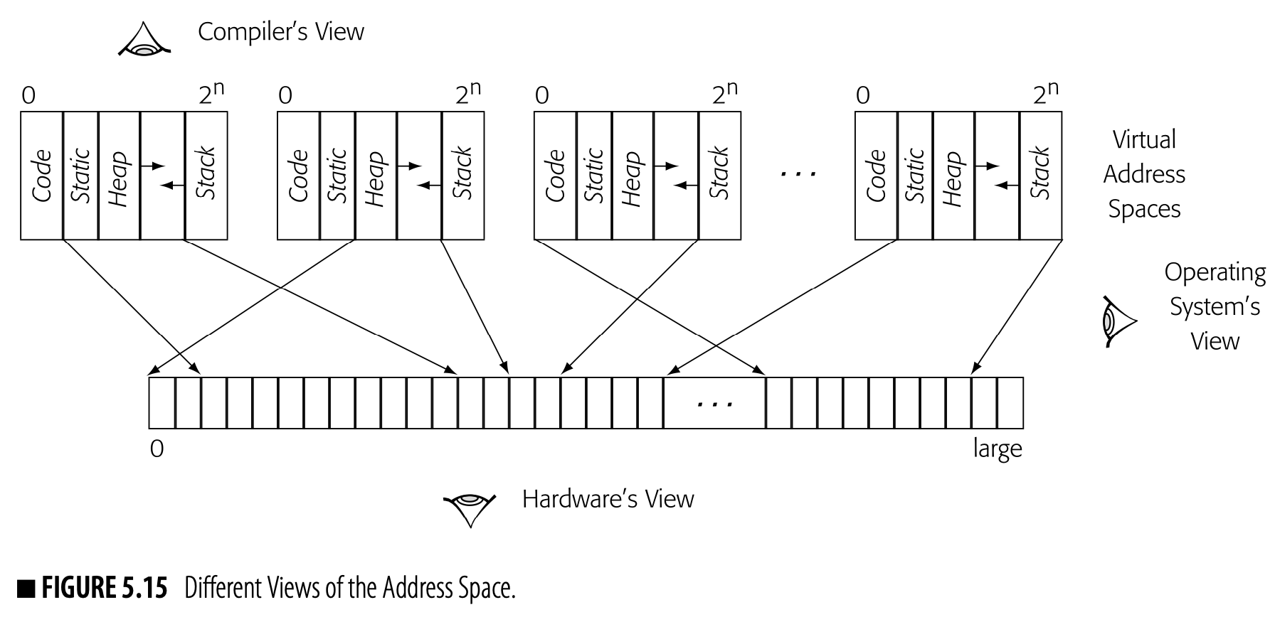
Page the fundamental unit of allocation in a virtual address space The operating system maps virtual pages into physical page frames.

A single virtual address space can occupy disjoint pages in the physical address space; thus, the addresses 100,000 and 200,000 in the program's virtual address space need not be 100,000 bytes apart in physical memory. In fact, the physical address associated with the virtual address 100,000 may be larger than the physical address associated with the virtual address 200,000. The mapping from virtual addresses to physical addresses is maintained cooperatively by the hardware and the operating system. It is, in almost all respects, beyond the compiler's purview.

5.6.3 Storage Assignment

Given the set of variables in a specific data area, the compiler must assign them each a storage location. If the compiler writer intends to maximize register use, then the compiler will first find each register-sized unambiguous value and assign it a unique virtual register (see Section 4.7.2). Next, it will assign each ambiguous value an offset from the start of the data area. Section 5.6.5 describes a method for laying out data areas while minimizing the impact of hardware alignment restrictions.

Internal Layout for Arrays

While arrays were added to $FORTR A N$ to model matrices in numerical calculations, they have many other uses.

Most programming languages include an array construct--a dimensioned aggregate structure in which all the members have the same type. During storage layout, the compiler needs to know where it will place each array. It must also understand when the size of that array is set and how to calculate its space requirements. These issues depend, in part, on the scheme used to lay out the array elements in memory.

While arrays were added to FORTRAN to model matrices in numerical calculations, they have many other uses.

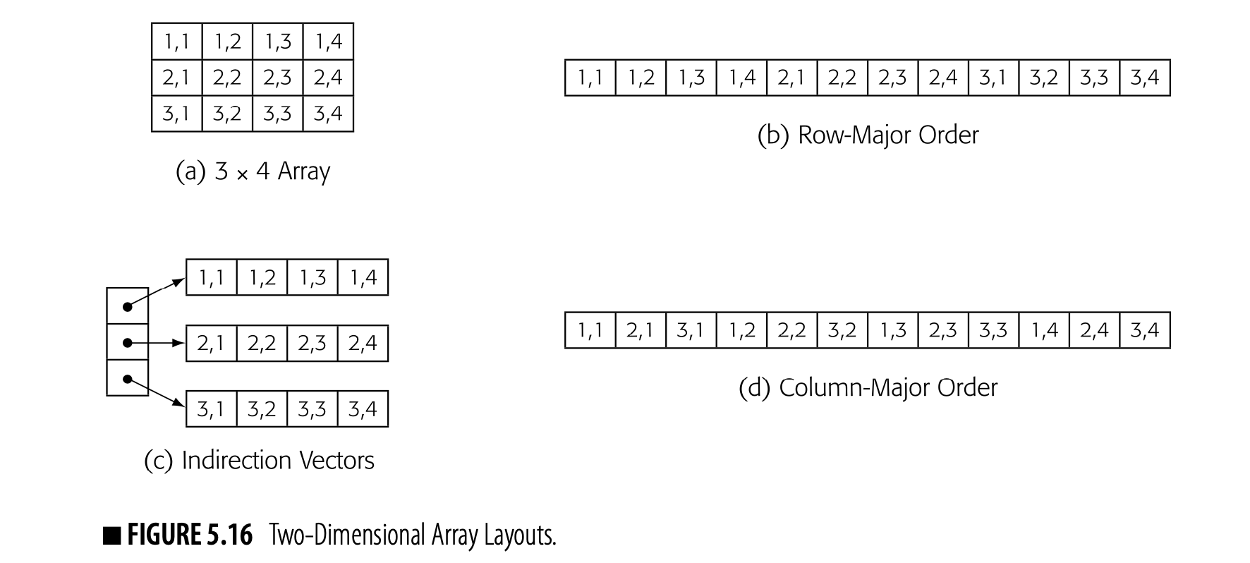The compiler can lay out a one-dimensional array, or vector, as a set of adjacent memory locations. Given the range of valid indices, from low to high, the vector will need $(high - low + 1) \times w$ contiguous bytes of storage, where $w$ is the width of an element in bytes. The address of $V [i]$ is just $\emptyset v + (i - low) \times w$ where $\emptyset v$ is the address of the first element of $V$ .

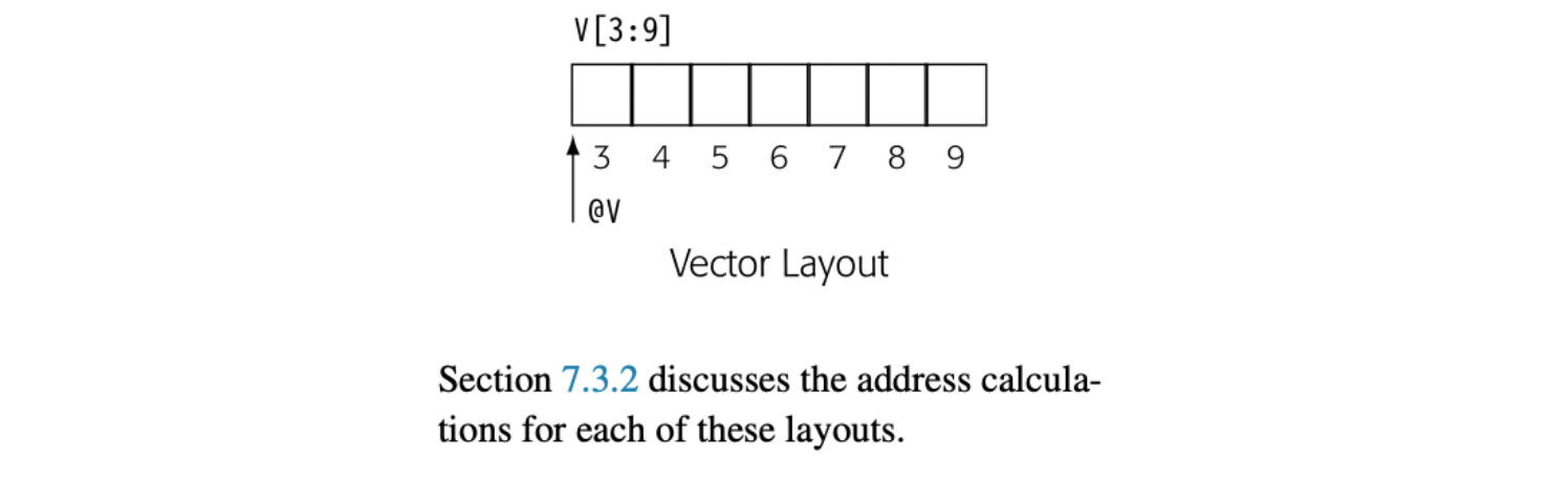With two or more dimensions, the language must specify an array layout. Fig. 5.16 shows three options that are used in practice. Panel (a) shows a conceptual view of a $3 \times 4$ array.

An array in row-major order is laid out as a series of rows, as shown in panel (b). Many languages use row-major order. Alternatively, an array that is in column-major order is laid out as a series of columns, as shown in panel (d). Fortran uses column-major order. If the array has $c$ columns and $r$ rows with elements of $w$ bytes, both of these layouts use $c \times r \times w$ bytes of contiguous storage.

The final option is to lay out the array as a series of indirection vectors, as shown in panel (c). JAVA uses this scheme. Here, the final dimension of the array is laid out in contiguous locations, and the other dimensions are represented with vectors of pointers. For an array with $c$ columns and $r$ rows, it requires $c \times r \times w$ space for the data, plus $r \times p$ space for the pointers, where $w$ is the size of an array element and $p$ is the size of a pointer. The individual rows and the column of pointers need not be contiguous.

Internal Layout for Strings

Section 7.6 discusses operations on strings.

Most programming languages support some form of string. Character strings are common; strings with elements of other types do occur. The representation is slightly more complex than that of a vector because a string variable might take on string values of different lengths at runtime. Thus, a string representation must hold the string's current content and the length of that content. It might also indicate the longest string that it can hold.

The glyph $b$ represents a blank.

Two common representations are a null-terminated string and a string with a length field. A null-terminated string, shown to the left, uses a vector of elements, with a designated end-of-string marker. C introduced this representation; other languages have followed.

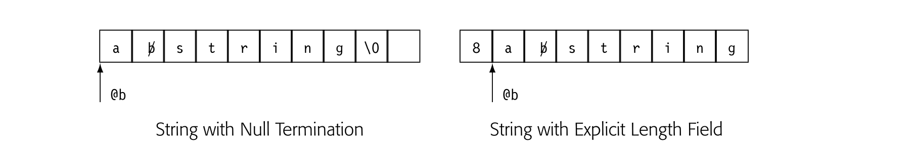
The explicit length representation, shown on the right, stores the value of the length in a separate field. These two layouts have slightly different space requirements; the null-terminated string requires an extra element to mark the string's end while the explicit length representation needs an integer large enough to hold the maximum string length.

The real difference between these representations lies in the cost of computing the string's length. In the null-terminated string, the cost is $O (n)$ where $n$ is the string's length, while the same operation is $O (1)$ in the explicit-length string. This difference carries into other operations that need to know the length, such as concatenation. It plays a critical role in range checking (see Section 7.3.3).

Internal Layout for Structures

The compiler must also perform layout for structures and objects. Most languages treat the interior of a structure declaration as a new scope. The programmer can use arbitrary names for the fields and scope rules will ensure the correct interpretation. Each field in a structure declaration allocates space within the structure; the compiler must assign each field an offset within the structure's representation.

Systems programming languages often fol- low declaration layout so that a program can interface with hardware defined lay- outs, such as device control blocks.

Programming languages differ as to whether or not the text of a structure declaration also defines the layout of the structure. Strong arguments exist for either choice. If the declaration dictates layout, then the compiler assigns offsets to the fields as declared. If the compiler controls structure layout, it can assign offsets within the structure to eliminate wasted space, using the technique for data-area layout.

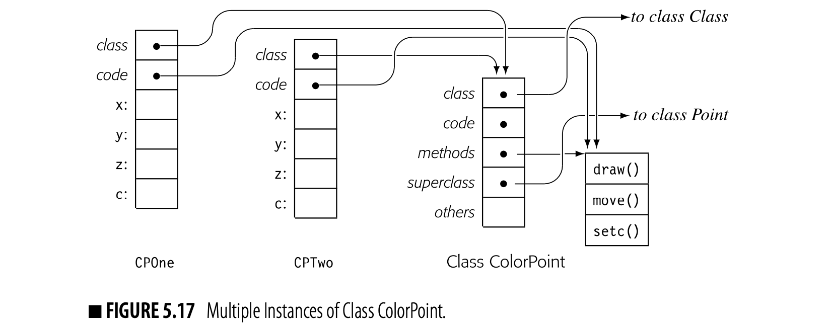
Internal Layout for Object Records

In an object-oriented language, each object has its own object record (OR). Because object lifetimes are irregular, ORs typically live on the heap. The OR holds the data members specified by the object's class, along with pointers to its class and, in many implementations, a vector of the class' methods. With inheritance, the OR must include data members inherited from its superclasses and access to code members of its superclasses.

The drawing in the margin shows an OR layout for an instance of class ColorPoint from Fig. 5.11. The OR has storage for each data member of the object, plus pointers to class ColorPoint's OR and to a vector of visible methods for ColorPoint. 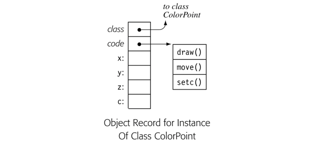The major complication in object layout arises from the fact that superclass methods should work on subclass objects. To ensure this interoperability, the subclass object layout must assign consistent offsets to data members from superclasses. With single-inheritance, the strategy of prefix layout achieves this goal. The subclass object layout uses the superclass object layout as a prefix. Data members from ancestors in the superclass chain retain consistent offsets; data members from the current class are added to the end of the OR layout.

To reduce storage requirements, most implementations store the method vector in the class' OR rather than keeping a copy in each object's OR. Fig. 5.17 shows the ORs for two instances of ColorPoint along with the class' OR. Linking the ORs for CP0ne and CPTwo directly to the method vector for ColorPoint reduces the space requirement without any direct cost. Of course, offsets in the method vectors must be consistent up the inheritance hierarchy chain; again, prefix layout works well for single inheritance environments.

DETALS MATTER In compiler construction, the details matter. As an example, consider two classes, $α$ and its subclass $β$ . When the compiler lays out $β$ 's object records, does it include private members of $α$ ? Since they are private, an object of class $β$ cannot access them directly.

An object of class $β$ will need those private members from $α$ if $α$ provides public methods that read or write those private members. Similarly, if the OR layout changes without them, the private members may be necessary to ensure that public members have the correct offsets in an OR of class $β$ (even if there is no mechanism to read their values).

To simplify lookup, the OR can contain a fully instantiated code vector, with pointers to both class and superclass methods.

Object Record Layout for Multiple Inheritance

Multiple inheritance complicates OR layout. The compiled code for a superclass method uses offsets based on the OR layout of that superclass. Different immediate superclasses may assign conflicting offsets to their members. To reconcile these competing offsets, the compiler must adopt a slightly more complex scheme: it must use different OR pointers with methods from different superclasses. 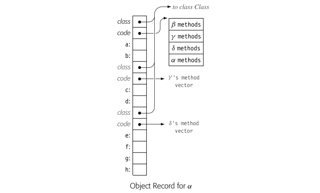Consider a class $α$ that inherits from multiple superclasses, $β$ , $γ$ , and $δ$ . To lay out the OR for an object of class $α$ , the implementation must first impose an order on $α$ 's superclasses--say $β$ , $γ$ , $δ$ . It then lays out the OR for class $α$ with the entire OR for $β$ , including class pointer and method vector, as a prefix to $α$ . Following that, it lays out the OR for $γ$ and, then, the OR for $δ$ . To this layout, it appends the data members of $α$ . It constructs a method vector by appending the inherited methods, in order by class, followed by any methods from $α$ . The drawing in the margin shows this layout, with the class pointers and method vectors for $β$ and $γ$ in the middle of the OR.

The drawing assumes that each class defines two data members: $β$ defines a and b; $γ$ defines c and d; $δ$ defines e and f; and $α$ defines g and h. The code vector for $α$ points to a vector that contains all of the methods that $α$ defines or inherits.

At runtime, a method from class $β$ will find all of the data members that it expects at the same offsets as in an object of class $β$ . Similarly, a method compiled for class $α$ will find the data members of $α$ at offsets known when the method was compiled.

Methods compiled for $β$ , $γ$ , or $δ$ cannot see members defined in $α$ . Thus, the code can adjust the OR pointer with impunity.

Methods compiled for $β$ , $γ$ , or $δ$ cannot see members defined in $α$ . Thus, the code can adjust the OR pointer with impunity.

For members of classes $γ$ or $δ$ , however, data members are at the wrong offset. The compiler needs to adjust the OR pointer so that it points to the appropriate point in the OR. Many systems accomplish this effect with a trampoline function. The trampoline function simply increments the OR pointer and then invokes the method; on return from the method, it decrements the OR pointer and returns.

5.6.4 Fitting Storage Assignment into Translation

The compiler writer faces a choice in translation. She can design the compiler to perform as much translation as possible during the syntax-driven phase, or she can design it to build an initial IR during the translation and rely on subsequent passes over the IR to complete the translation. The timing of storage layout plays directly into this choice.

The compiler writer can use a mid- production action in a rule similar to Body → Decls Execs where Decls derives declarations and Execs derives executable statements.

Some languages require that all variables be declared before any executable statement appears. The compiler can gather all of the type and symbol information while processing declarations. Before it processes the first executable statement, it can perform storage layout, which allows it to generate concrete code for references.
If the language requires declarations, but does not specify an order, the compiler can build up the symbol table during parsing and emit IR with abstract references. After parsing, it can perform type inference followed by storage layout. It can then refine the IR and make the references more concrete.
If the language does not require declarations, the compiler must build an IR with abstract references. The compiler can then perform some more complex (probably iterative) type inference on the IR, followed by storage layout. Finally, it can refine the IR and make the references more concrete.

The choice between these approaches depends on the rules of the source language and the compiler writer's preference. A multipass approach may simplify the code in the compiler itself.

5.6.5 Alignment Restrictions and Padding

Alignment restriction Most processors restrict the alignment of values by their types. For example, an eight-byte integer may need to begin at an address $a$ such that $a$ mod $8 = 0$ .

Instruction set architectures restrict the alignment of values. (Assume, for this discussion, that a byte contains eight bits and that a word contains four bytes.) For each hardware-supported data type, the ISA may restrict the set of addresses where a value of that type may be stored. For example, a 32-bit floating-point number might be restricted to begin on a word, or 32-bit, boundary. Similarly, a 64-bit integer might be restricted to a doubleword, or 64-bit boundary.

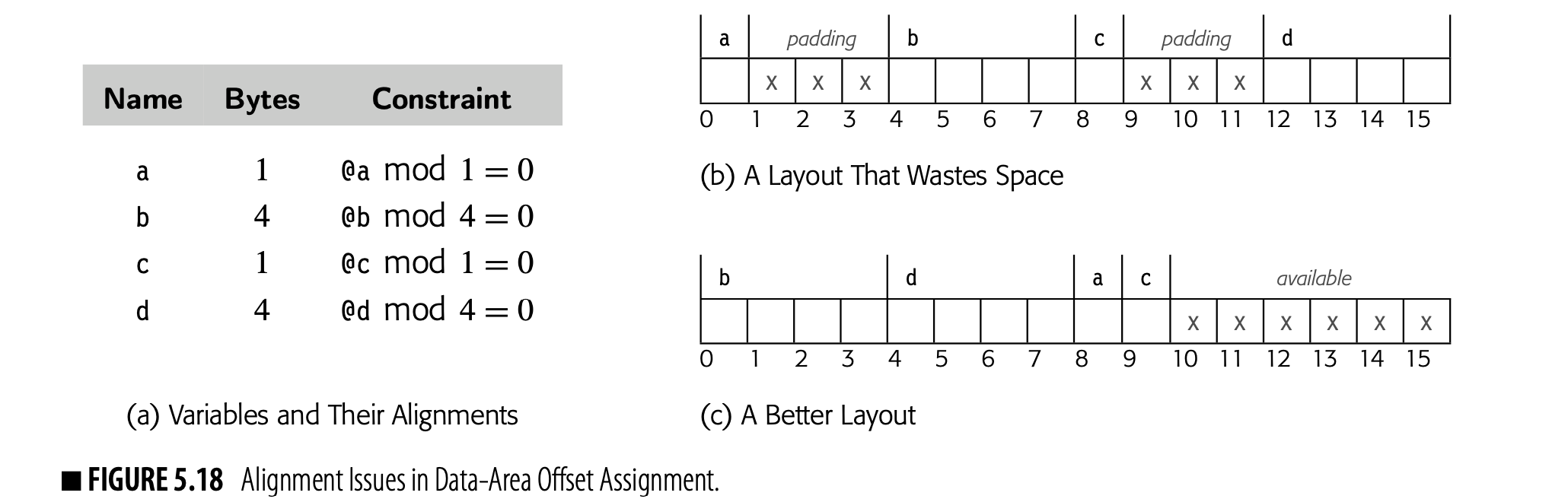
The compiler has two mechanisms to enforce alignment restrictions. First, it can control the alignment of the start of each data area. Most assembly languages have directives to enforce doubleword or quadword alignment at the start of a data area. Such pseudooperations ensure that each data area starts at a known alignment.

Second, the compiler controls the internal layout of the data area; that is, it assigns an offset to each value stored in the data area. It can ensure, through layout, that each value has the appropriate alignment. For example, a value that needs doubleword alignment must have an offset that is evenly divisible by eight.

Consider a variable $x$ stored at offset in a data area that starts at address base. If base is quadword aligned, then base $MOD 16 = 0$ . If offset $MOD 8 = 0$ , then the address of $x$ , which is base $+$ offset, is doubleword aligned - that is (base $+$ offset) $MOD 8 = 0$ .

As the compiler lays out a data area, it must satisfy all of the alignment restrictions. To obtain proper alignment, it may need to insert empty space between values. Fig. 5.18(a) shows the lengths and constraints for a simple four-variable example. Panel (b) shows the layout that results if the compiler assigns them offsets in alphabetical order. It uses sixteen bytes and wastes six bytes in padding. Panel (c) shows an alternative layout that uses ten bytes with no padding. In both cases, some space may be wasted before the next entity in memory.

To create the layout in panel (c), the compiler can build a list of names for a given data area and sort them by their alignment restrictions, from largest to smallest alignment boundary. Next, it can assign offsets to the names in sorted order. If it must insert padding to reach the alignment boundary for the next name, it may be able to fill that space with small-boundary names from the end of the list.

SECTION REVIEW

The compiler must decide, for each runtime entity, where in storage it will live and when its storage will be allocated. The compiler bases its decision on the entity’s lifetime and its visibility. It classifies names into storage classes. For objects with predictable lifetimes, the storage class guides these decisions.

The compiler typically places items with unpredictable lifetimes on the runtime heap. Heap-based entities are explicitly allocated; typically, references to heap-based entities involve a level of indirection through a variable with a regular lifetime.

REVIEW QUESTIONS

In C, a file might contain both file static and procedure static variables. Does the compiler need to create separate data areas for these two dis- tinct classes of visibility?

Consider the short fragment of C code shown in the margin. It names three values, a, b, and *b. Which of these values are ambiguous? Which are unambiguous?

5.7 ADVANCED TOPICS

This chapter has focused on the mechanism of syntax-driven translation and its uses in building a compiler. As use cases, it has discussed translation of expressions and if–then–else statements, models of the source program’s naming environment, a simple approach to type checking, and storage lay- out. This section expands on three issues.

The first subsection looks at the relationship between the direction of recur- sion in a grammar and associativity. The second subsection discusses the interaction between language design and type inference and checking. The final subsection looks briefly at the interaction between cache offsets and performance.

5.7.1 Grammar Structure and Associativity

In Chapter 3, we saw left-recursive and right-recursive variants of the ex- pression grammar, along with a transformation to eliminate left-recursion. In that discussion, we noted that the transformation preserves associativity. This subsection explores the relationship between recursion, associativity, IR structure, and parse stack depth. Consider the following simple gram- mars, for addition over names. Given an input expression $a + b + c + d + e$ , the two grammars lead to significantly different ASTs, as shown in the margin. With extreme values, these trees can evaluate to measurably different results.

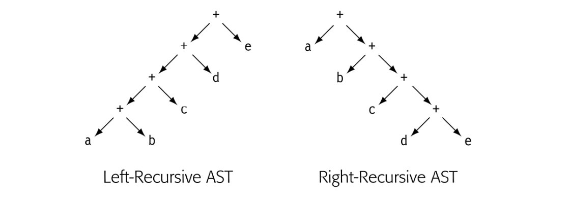
A postorder evaluation of the AST from the left-recursive grammar will evaluate to $(((a + b) + c) + d) + e$ , while the right-recursive version will evaluate to $(((d + e) + c) + b) + a$ . With addition, which is both commutative and associative, the numerical difference in these sums will only arise with extremely large or small values.

With an $LL (1)$ parser generator, where left recursion is not an option, the compiler writer can obtain left-associativity by writing the left-recursive grammar and using the transformation to convert left-recursion to rightrecursion. With an $L R (1)$ parser generator, the compiler writer can choose either left or right recursion to suit the circumstances.

Stack Depth

In general, left recursion can lead to smaller stack depths. Consider what happens when an LR(1) parser processes the expression $a + b + c + d + e$ with each of our grammars shown earlier.

Left-Recursive Grammar This grammar shifts a onto the stack and immediately reduces it to Expr. Next, it shifts + and b onto the stack and reduces $E x p r + b$ to Expr. It continues, shifting $a +$ and a name onto the stack and reducing the left context to Expr. When it hits the end of the string, the maximum stack depth has been three and the average depth has been 1.8 .
Right-Recursive Grammar This grammar first shifts all the tokens onto the stack $(a, +, b, +, c, +, d, +, e)$ . It then reduces e to $E x p r$ , using the second rule. It then performs a series of four reduces with the first production: $d + Exp r$ to $Expr$ , $c + Exp r$ to $E x p r$ , $b + E x p r$ to $E x p r$ , and $a + E x p r$ to $E x p r$ . When it finishes, the maximum stack depth has been nine and the average stack depth has been 4.8 .

The right-recursive grammar requires more stack space; its maximum stack depth is bounded only by the length of the expression. By contrast, the maximum stack depth with the left-recursive grammar depends on the gram- mar rather than the input stream.

Building Lists

The same issues arise with lists of elements, such as the list of statements in a block. The compiler writer can use either left recursion or right recursion in the grammar. The left-recursive grammar uses a bounded amount of stack space while the right-recursive grammar uses stack space proportional to the length of the list. For short lists, stack space is not a problem. For long lists--say a block with hundreds or thousands of statements--the difference can be dramatic. This observation suggests that the compiler writer should use the left-recursive grammar.

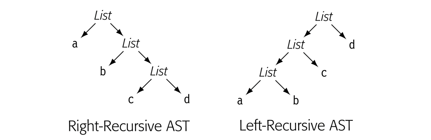The problem with this approach arises when the compiler builds a data structure to represent the list. Consider a simple abstract syntax tree for a four element list: (a b c d). The AST from the right-recursive grammar reflects our intuitions about the statement list; a is first and d is last. The tree from the left-recursive grammar represents the same information; the statements are ordered correctly left to right. The nesting order, however, is somehow less intuitive than that for the right-recursive version of the AST. The code to traverse the list becomes less obvious, as well.

In many cases, the compiler writer will want to use the left-recursive grammar for its bounded stack space but build the AST that would naturally result from the right-recursive grammar. The answer is to build a list constructor that adds successive elements to the end of the list. A straightforward implementation of this idea would walk the list on each reduction, which makes the constructor take $O (n^{2})$ time, where $n$ is the length of the list.

With the right set of list constructors, the compiler writer can arrange to build the right-recursive AST from the left-recursive grammar. Consider the following syntax-driven framework: 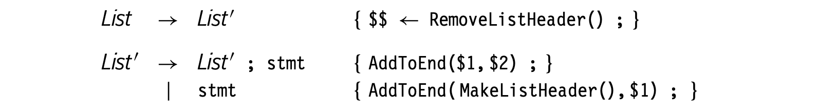The framework uses three helper functions.

We developed this framework for an ILOC parser written in bison. The original right- recursive version overflowed the parse stack on inputs with more than 64,000 operations.

MakeListHeader() builds a header node that contains pointers to the start and end of a list. It returns a pointer to the header node. RemoveListHeader(x) takes as input a header node x. It returns x’s start- of-list pointer and discards the header node. AddToEnd(x, y) takes as input a header node x and an item y. It creates a new List node and makes y its left child and nil its right child. It then uses x’s end-of-list pointer to add the new List node to the end of the list. Finally, it returns x.

Each of these functions can be implemented so that it uses $O (1)$ time. They work together to build and maintain both the header node and the list. The framework adds the production $L i s t \to L i s t'$ to create a point in the computation where it can discard the header node. The AST that it builds differs slightly from the one shown earlier; as shown in the margin, it always has a nil as the right child of the final List node.

5.7.2 HarderProblemsinTypeInference

Strongly typed, statically checked languages can help the programmer produce valid programs by detecting large classes of erroneous programs. The same features that expose errors can improve the compiler's ability to generate efficient code for a program by (1) eliminating runtime checks or (2) exposing situations where the compiler can specialize code for some construct to eliminate cases that cannot occur at runtime. These advantages account, in part, for the growing role of type systems in programming languages.

Our examples, however, make assumptions that do not hold in all programming languages. For example, we assumed that variables and procedures are declared--the programmer writes down a concise and binding specification for each name. Varying these assumptions can radically change the nature of both the type-checking problem and the strategies that the compiler can use to implement the language.

Some programming languages either omit declarations or treat them as optional information. PYTHON and SCHEME programs lack declarations for variables. SMALLtalk programs declare classes, but an object's class is determined only when the program instantiates that object. Languages that support separate compilation--compiling procedures independently and combining them at link time to form a program--may not require declarations for independently compiled procedures.

In the absence of declarations, type checking is harder because the compiler must rely on contextual clues to determine the appropriate type for each name. For example, if the compiler sees an array reference a[i], that usage might constrain the type of i. The language might allow only integer subscripts; alternatively, it might allow any type that can be converted to an integer.

Typing rules are specified by the language definition. The specific details of those rules determine how difficult it is to infer a type for each variable. This, in turn, has a direct effect on the strategies that a compiler can use to implement the language.

Type-Consistent Uses and Constant Function Types

Consider a declaration-free language that requires consistent uses for variables and functions. The compiler can assign a general type to each name and narrow that type by examining uses of the name in context. For example, the statement a $\leftarrow$ b x 3.14159 suggests that a and b are numbers and that a must have a type that allows it to hold a decimal number. If b also appears in contexts where an integer is expected, such as an array reference c[b], then the compiler must choose between a decimal number (for b x 3.14159) and an integer (for c[b]). With either choice, one of the uses will need a conversion.

If functions have return types that are both known and constant--that is, a function _f_ee always returns the same type--then the compiler can solve the type inference problem with an iterative fixed-point algorithm operating over a lattice of types.

Type-Consistent Uses and Unknown Function Types

Map can also handle functions with multi- ple arguments. To do so, it takes multiple argument lists and treats them as lists of arguments, in order.

If the type of a function varies with the function's arguments, then the problem of type inference becomes more complex. This situation arises in SCHEME, for example, where the library function map takes as arguments a function and a list. It returns the result of applying the function argument to each element of the list. That is, if the argument function takes type $α$ to $β$ , then map takes a list of $α$ to a list of $β$ . We would write its type signature as Since map's return type depends on the types of its arguments, a property known as parametric polymorphism, the inference rules must include equations over the space of types. (With known, constant return types, functions return values in the space of types.) With this addition, a simple iterative fixed-point approach to type inference is not sufficient.

The classic approach to checking these more complex systems relies on unification, although clever type-system design and type representations can enable use of simpler or more efficient techniques.

Dynamic Changes in Type

If a variable's type can change during execution, other strategies may be required to discover where type changes occur and to infer appropriate types. In principle, a compiler can rename the variables so that each definition site corresponds to a unique name. It can then infer types for those names based on the context provided by the operation that defines each name.

To infer types successfully, such a system would need to handle points in the code where distinct definitions must merge due to the convergence of different control-flow paths, as with $ϕ$ -functions in static single assignment form (see Sections 4.6.2 and 9.3). If the language includes parametric polymorphism, the type-inference mechanism must handle it, as well.

The classic approach to implementing a language with dynamically changing types is to fall back on interpretation. LISP, SCHEME, SMALLTLK, and aPL all face this challenge. The standard implementation practice for these languages involves interpreting the operators, tagging the data with their types, and checking for type errors at runtime.

In aPL, the expression axb can multiply integers the first time it executes and multiply multidimensional arrays of floating-point numbers the next time. This feature led to a body of research on check elimination and check motion. The best aPL systems avoided many of the checks that a naive interpreter would need.

5.7.3 Relative Offsets and Cache Performance

The widespread use of cache memories has subtle implications for the layout of variables in memory. If two values are used in proximity in the code, the compiler would like to ensure that they can reside in the cache at the same time. This can be accomplished in two ways. In the best situation, the two values would share a single cache block, to guarantee that the values are always fetched into cache together. If they cannot share a cache block, the compiler would like to ensure that the two variables map to different cache lines. The compiler can achieve this by controlling the distance between their addresses.

If we consider just two variables, controlling the distance between them seems manageable. When all the active variables are considered, however, the problem of optimal arrangement for a cache is NP-complete. Most variables have interactions with many other variables; this creates a web of relationships that the compiler may not be able to satisfy concurrently. If we consider a loop that uses several large arrays, the problem of arranging mutual noninterference becomes even worse. If the compiler can discover the relationship between the various array references in the loop, it can add padding between the arrays to increase the likelihood that the references hit different cache lines and, thus, do not interfere with each other.

A PRIMER ON CACHE MEMORIES

One technique that architects use to bridge the gap between processor speed and memory speed is the use of cache memories. A cache is a small, fast memory placed between the processor and main memory. The cache is divided into a set of equal-sized frames. Each frame has a tag that holds enough of the main-memory address to identify the contents of the frame.

The hardware automatically maps memory locations to cache frames. The simplest mapping, used in a direct-mapped cache, computes the cache address as the main memory address modulo the size of the cache. This partitions the memory into a linear set of blocks, each the size of a cache frame. A line is a memory block that maps to a frame. At any point in time, each cache frame holds a copy of the data from one of its blocks. Its tag field holds the address in memory where that data normally resides.

On each read from memory, the hardware first checks to see if the requested word is already in its cache frame. If so, it returns the requested bytes to the processor. If not, (1) the block currently in the frame is evicted, (2) the requested block is fetched into the cache, and (3) the requested bytes are returned to the processor.

Some caches use more complex mappings. A set-associative cache uses multiple frames per cache line, typically two or four frames per line. A fully associative cache can place any block in any frame. Both of these schemes use an associative search over the tags to determine if a block is in the cache. Associative schemes use a policy to determine which block to evict. Common schemes are random replacement and least-recently-used replacement.

In practice, the effective memory speed is determined by memory bandwidth, cache block length, the ratio of cache speed to memory speed, and the ratio of cache hits to cache misses. From the compiler’s perspective, the first three are fixed. Compiler-based efforts to improve memory performance focus on increasing the ratio of cache hits to cache misses.

Some architectures provide instructions for a program to give the cache hints as to when specific blocks should be brought into memory (prefetched) and when they can be discarded (flushed).

As we saw previously, the mapping of the program’s virtual address space to the hardware’s physical address space need not preserve the distance be- tween specific variables. Carrying this thought to its logical conclusion, the reader should ask how the compiler can ensure anything about relative off- sets that are larger than the size of a virtual-memory page. The processor’s cache may use either virtual addresses or physical addresses in its tag fields. A virtually addressed cache preserves the distance between values in the vir- tual space; the compiler may force noninterference between large objects. With a physically addressed cache, the distance between two locations in different pages is determined by the page map (unless cache size ≤ page size). Thus, the compiler’s decisions about memory layout have little, if any, effect, except within a single page. In this situation, the compiler should fo- cus on placing objects that are referenced together into the same page and, if possible, the same cache line.

5.8 Summary and Perspective

The real work of compilation is translation: mapping constructs in the source language to operations on the target machine. The compiler's front end builds an initial model of the program: an IR representation and a set of ancillary structures. This chapter explored syntax-driven translation, a mechanism that lets the compiler writer specify actions to be performed when the front end recognizes specific syntactic constructs. The compiler writer ties those actions to grammar productions; the compiler executes them when it recognizes the production.

We suspect that attribute grammar systems have failed to win an audience because of the lack of a widely available, well- implemented, easy-to-use system.

yacc and bison won the day not because they are elegant, but because they were distributed with UNIX and they worked

Formal techniques have automated much of scanner and parser construction. In translation, most compilers rely on the ad-hoc techniques of syntax-driven translation. While researchers have developed more formal techniques, such as attribute grammar systems, those systems have not been widely adopted. The syntax-driven techniques are largely ad-hoc; it takes some practice for a compiler writer to use them effectively. This chapter captures some of that experience.

To perform translation, the compiler must build up a base of knowledge that is deeper than the syntax. It must use the language's type system to infer a type for each value that the program computes and use that information to drive both error detection and automatic type conversions. Finally, the compiler must compute a storage layout for the code that it sees; that storage layout must be consistent with and compatible with the results of other compilations of related code.

Chapter Notes

The material in this chapter is an amalgam of accumulated knowledge drawn from practices that began in the late 1950s and early 1960s.

The concepts behind syntax-driven translation have always been a part of the development of real parsers. Irons, describing an early ALGOL-60 compiler, clearly lays out the need to separate a parser's actions from the description of its syntax [214]; he describes the basic ideas behind syntax-driven translation. The same basic ideas were undoubtedly used in contemporary operator precedence parsers.

The specific notation used to describe syntax-driven actions was introduced by Johnson in the yacc system [216]. This notation has been carried forward into many more recent systems, including the Gnu project's bison parser generator.

Type systems have been an integral part of programming languages since the original Fortran compiler. While the first type systems reflected the resources of the underlying machine, deeper levels of abstraction soon appeared in type systems for languages such as ALGOL 68 and SIMULA-67. The theory of type systems has been actively studied for decades, producing a string of languages that embodied important principles. These include RUSSELL[49] (parametric polymorphism), CLU[256] (abstract data types), SMALLtalk[172] (subtyping through inheritance), and ML[274] (thorough and complete treatment of types as first-class objects). Cardelli has written an excellent overview of type systems [76]. The APL community produced a series of classic papers that dealt with techniques to eliminate runtime checks [1, 38, 273, 361].

Most of the material on storage layout has developed as part of programming language specifications. Column-major order for arrays appeared in early Fortran systems [27, 28] and was codified in the Fortran 66 standard. Row-major order has been used since the 1950s.

Chapter 9. Data-Flow Analysis

ABSTRACT

Compilers analyze the IR form of the program in order to identify opportunities where the code can be improved and to prove the safety and profitability of transformations that might improve that code. Data-flow analysis is the classic technique for compile-time program analysis. It allows the compiler to reason about the runtime flow of values in the program.

This chapter explores iterative data-flow analysis, based on a simple fixed-point algorithm. From basic data-flow analysis, it builds up to construction of static single-assignment (ssa) form, illustrates the use of ssa form, and introduces interprocedural analysis.

KEYWORDS Data-Flow Analysis, Dominance, Static Single-Assignment Form, Constant Propagation

9.1 Introduction

As we saw in Chapter $8$ , optimization is the process of analyzing a program and transforming it in ways that improve its runtime behavior. Before the compiler can improve the code, it must locate points in the program where changing the code is likely to provide improvement, and it must prove that changing the code at those points is safe. Both of these tasks require a deeper understanding of the code than the compiler's front end typically derives. To gather the information needed to find opportunities for optimization and to justify those optimizations, compilers use some form of static analysis.

In general, static analysis involves compile-time reasoning about the runtime flow of values. This chapter explores techniques that compilers use to analyze programs in support of optimization.

Conceptual Roadmap

Compilers use static analysis to determine where optimizing transformations can be safely and profitably applied. In Chapter $8$ , we saw that optimizations operate on different scopes, from local to interprocedural. Ingeneral, a transformation needs analytical information that covers at least as large a scope as the transformation; that is, a local optimization needs at least local information, while a whole-procedure, or global, optimization needs global information.

Static analysis generally begins with control-flow analysis; the compiler builds a graph that represents the flow of control within the code. Next, the compiler analyzes the details of how values flow through the code. It uses the resulting information to find opportunities for improvement and to prove the safety of transformations. Data-flow analysis was developed to answer these questions.

Static single-assignment (SSA) form is an intermediate representation that unifies the results of control-flow and data-flow analysis in a single sparse data structure. It has proven useful in both analysis and transformation and has become a standard ir used in both research and production compilers.

Overview

Chapter 8 introduced the subject of analysis and transformation of programs by examining local methods, regional methods, global methods, and interprocedural methods. Value numbering is algorithmically simple, even though it achieves complex effects; it finds redundant expressions, simplifies code based on algebraic identities and zero, and propagates known constant values. By contrast, finding an uninitialized variable is conceptually simple, but it requires the compiler to analyze the entire procedure to track definitions and uses.

Join point In a CFG, a join point is a node that has multiple predecessors.

The difference in complexity between these two problems lies in the kinds of control flows that they encounter. Local and superlocal value numbering deal with subsets of the control-flow graph (CFG) that form trees (see Sections 8.4.1 and 8.5.1). To analyze the entire procedure, the compiler must reason about the full cfg, including cycles and join points, which both complicate analysis. In general, methods that only handle acyclic subsets of the cfg are amenable to online solutions, while those that deal with cycles in the cfg require offline solutions--the entire analysis must complete before rewriting can begin.

Static analysis analysis performed at compile time or link time

Dynamic analysis analysis performed at runtime, perhaps in a JIT or specialized self-modifying code

Static analysis, or compile-time analysis, is a collection of techniques that compilers use to prove the safety and profitability of a potential transformation. Static analysis over single blocks or trees of blocks is typically straightforward. This chapter focuses on global analysis, where the cfg can contain both cycles and join points. It mentions several problems in interprocedural analysis; these problems operate over the program's call graph or some related graph.

In simple cases, static analysis can produce precise results--the compiler can know exactly what will happen when the code executes. If the compiler can derive precise information, it might determine that the code evaluates to a known constant value and replace the runtime evaluation of an expression or function with an immediate load of the result. On the other hand, if the code reads values from any external source, involves even modest amounts of control flow, or encounters any ambiguous memory references, such as pointers, array references, or call-by-reference parameters, then static analysis becomes much harder and the results of the analysis are less precise.

This chapter begins with classic problems in data-flow analysis. We focus on an iterative algorithm for solving these problems because it is simple, robust, and easy to understand. Section 9.3 presents an algorithm for constructing SSA form for a procedure. The construction relies heavily on results from data-flow analysis. The advanced topics section explores the notion of flow-graph reducibility, presents a data structure that leads to a faster version of the dominator calculation, and provides an introduction to interprocedural data-flow analysis.

A Few Words About Time

The compiler analyzes the program to determine where it can safely apply transformations to improve the program. This static analysis either proves facts about the runtime flow of control and the runtime flow of values, or it approximates those facts. The analysis, however, takes place at compile time. In a classical ahead-of-time compiler, analysis occurs before any code runs.

Some systems employ compilation techniques at runtime, typically in the context of a just-in-time (JIT) compiler (see Chapter 14). With a JIT, the analysis and transformation both take place during runtime, so the cost of optimization counts against the program's runtime. Those costs are incurred on every execution of the program.

9.2 Iterative Data-Flow Analysis

Forward problem a problem in which the facts at a node n are computed based on the facts known for n’s CFG predecessors

Backward problem a problem in which the facts at a node n are computed based on the facts known for n’s CFG successors.

Compilers use data-flow analysis, a set of techniques for compile-time reasoning about the runtime flow of values, to locate opportunities for optimization and to prove the safety of specific transformations. As we saw with live analysis in Section 8.6.1, problems in data-flow analysis take the form of a set of simultaneous equations defined over sets associated with the nodes and edges of a graph that represents the code being analyzed. Live analysis is formulated as a global data-flow problem that operates on the control-flow graph (CFG) of a procedure. In this section, we will explore global data-flow problems and their solutions in greater depth. We will focus on one specific solution technique: an iterative fixed-point algorithm. It has the advantages of simplicity, speed, and robustness. We will first examine a simple forward data-flow problem, dominators in a flow graph. For a more complex example, we will return to the computation of LiveOut sets, a backward data-flow problem.

9.2.1 Dominance

Dominance In a flow graph with entry node $b_{0}$ , node $b_{i}$ dominates node $b_{j}$ , written $b_{i} ≫ b_{j}$ , if and only if $b_{i}$ lies on all paths from $b_{0}$ to $b_{j}$ . By definition, $b_{i} ≫ b_{i}$ .

Many optimization techniques must reason about the structural properties of the underlying code and its CFG. A key tool that compilers use to reason about the shape and structure of the CFG is the notion of dominance. Compilers use dominance to identify loops and to understand code placement. Dominance plays a key role in the construction of SSA form.

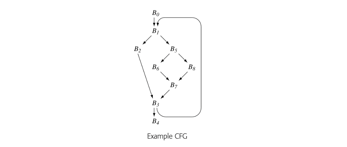
Many algorithms have been proposed to compute dominance information. This section presents a simple data-flow problem that annotates each CFG node $b_{i}$ with a set Dom( $b_{i}$ ). A node's Dom set contains the names of all the nodes that dominate $b_{i}$ .

To make the notion of dominance concrete, consider node $B_{6}$ in the CFG shown in the margin. Every path from the entry node, $B_{0}$ , to $B_{6}$ includes $B_{0}$ , $B_{1}$ , $B_{5}$ , and $B_{6}$ , so Dom( $B_{6}$ ) is ${B_{0}, B_{1}, B_{5}, B_{6}}$ . The table in the margin shows all of the Dom sets for the CFG.

For any CFG node $n$ , one $m \in DOM (n)$ , $m \neq = n$ , will be closer to $n$ in the CFG than any other $x \in DOM (n)$ , $x \neq = n$ . That node, $m$ , is the immediate dominator of $n$ , denoted IDom( $n$ ). By definition, a flow graph's entry node has no immediate dominator.

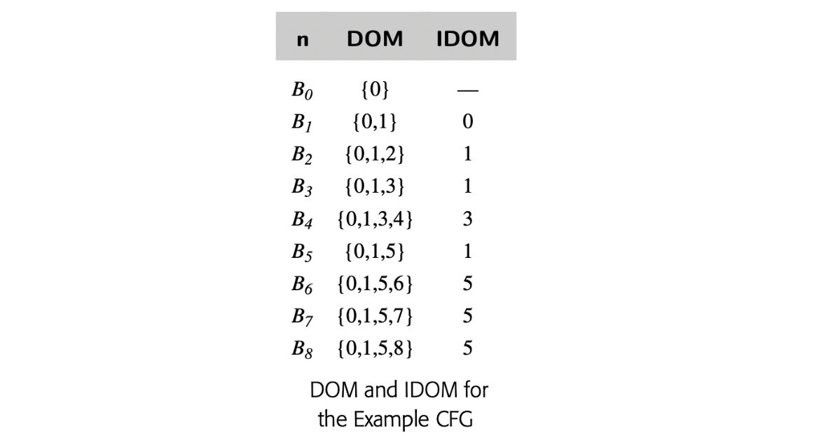
The following equations both define the Dom sets and form the basis of a method for computing them: 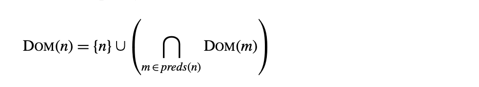To provide initial values, the compiler sets: 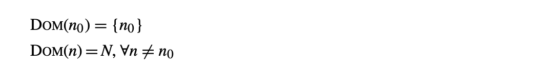where $N$ is the set of all nodes in the CFG. Given an arbitrary flow graph--that is, a directed graph with a single entry and a single exit--the equationsspecify the Dom set for each node. At each join point in the CFG, the equations compute the intersection of the Dom sets along each entering path. Because they specify Dom( $n$ ) as a function of $n$ 's predecessors, denoted $preds (n)$ , information flows forward along edges in the CFG. Thus, the equations create a forward data-flow problem.

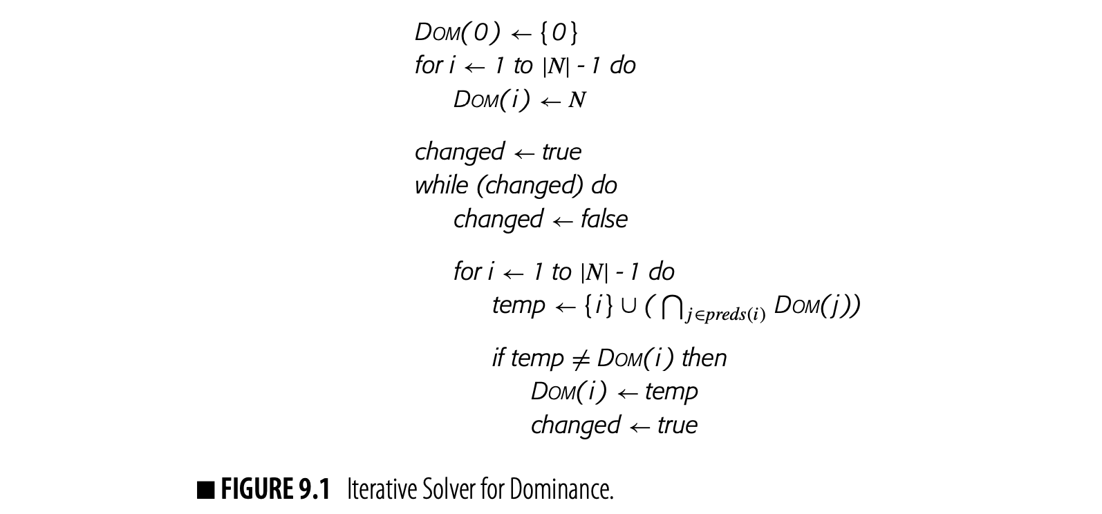
To solve the equations, the compiler can use the same three-step process used for live analysis in Section 8.6.1. It must (1) build a CFG, (2) gather initial information for each block, and (3) solve the equations to produce the Dom sets for each block. For Dom, step 2 is trivial; the computation only needs to know the node numbers.

Fig. 9 shows a round-robin iterative solver for the dominance equations. It considers the nodes in order by their CFG name, $B_{0}$ , $B_{I}$ , $B_{2}$ , and so on. It initializes the Dom set for each node, then repeatedly recomputes those Dom sets until they stop changing.

Fig. 2 shows how the values in the Dom sets change as the computation proceeds. The first column shows the iteration number; iteration zero shows the initial values. Iteration one computes correct Dom sets for any node with a single path from $B_{0}$ , but computes overly large Dom sets for $B_{3}$ , $B_{4}$ , and $B_{7}$ . In iteration two, the smaller Dom set for $B_{7}$ corrects the set for $B_{3}$ , which, in turn shrinks Dom( $B_{4}$ ). Similarly, the set for $B_{8}$ corrects the set for $B_{7}$ . Iteration three shows that the algorithm has reached a fixed point.

Three critical questions arise regarding this solution procedure. First, does the algorithm halt? It iterates until the Dom sets stop changing, so the argument for termination is not obvious. Second, does it produce correct Dom sets? The answer is critical if we are to use Dom sets in optimizations. Finally, how fast is the solver? Compiler writers should avoid algorithms that are unnecessarily slow.

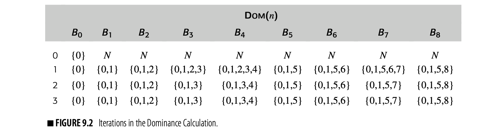
Termination

Iterative calculation of the Dom sets halts because the sets that approximate Dom shrink monotonically throughout the computation. The algorithm initializes Dom $(n_{0})$ to ${0}$ , and initializes the Dom sets for all other nodes to $N$ , the set of all nodes. A Dom set can be no smaller than ${0}$ and can be no larger than $N$ . Careful reasoning about the while loop shows that a Dom set, say Dom $(n_{i})$ , cannot grow from iteration to iteration. Either it shrinks, as the Dom set of one of its predecessors shrinks, or it remains unchanged.

The while loop halts when it makes a pass over the nodes in which no Dom set changes. Since the Dom sets can only change by shrinking and those sets are bounded in size, the while loop must eventually halt. When it halts, it has found a fixed point for this particular instance of the Dom computation.

Correctness

Recall the definition of dominance. Node $n_{i}$ dominates $n_{j}$ if and only if every path from the entry node $n_{0}$ to $n_{j}$ contains $n_{i}$ . Dominance is a property of paths in the CFG.

Dom $(n_{j})$ contains $i$ if and only if $i \in Dom (n_{k})$ for all $k \in preds (j)$ , or if $i = j$ . The algorithm computes Dom $(n_{j})$ as $j$ plus the intersection of the Dom sets of all $n_{j}$ 's predecessors. How does this local computation over individual edges relate to the dominance property, which is defined over all paths through the CFG?

Meet operator In the theory of data-flow analysis, the meet $o p er a t or (\land)$ is used to combine facts at a join point in the CFG. In the $D OM$ equations, the meet operator is set intersection.

The Dom sets computed by the iterative algorithm form a fixed-point solution to the equations for dominance. The theory of iterative data-flow analysis, which is beyond the scope of this text, assures us that a fixed point exists for these particular equations and that the fixed point is unique [221]. This "all-paths" formulation of Dom describes a fixed-point for the equations, called the meet-over-all-paths solution. Uniqueness guarantees that the fixed point found by the iterative algorithm is identical to the meet-over-all-paths solution.

Efficiency

Postorder number a labeling of the graph’s nodes that corre- sponds to the order in which a postorder traversal would visit them

Because the fixed-point solution to the Dom equations for a specific CFG is unique, the solution is independent of the order in which the solver computes those sets. Thus, the compiler writer is free to choose an order of evaluation that improves the analyzer's running time.

The compiler can compute RPO numbers in a postorder traversal if it starts a counter at $∣ N ∣ - 1$ and decrements the counter as it visits and labels each node.

A $reverse postorder$ (RPO) traversal of the graph is particularly effective for forward data-flow problems. If we assume that the postorder numbers run from zero to $∣ N ∣$ - 1, then a node's rpo number is simply $∣ N ∣$ - 1 minus that node's postorder number. Here, $N$ is the set of nodes in the graph.

An RPO traversal visits as many of a node's predecessors as possible, in a consistent order, before visiting the node. (In a cyclic graph, a node's predecessor may also be its descendant.) A postorder traversal has the opposite property; for a node $n$ , it visits as many of $n$ 's successors as possible before visiting $n$ . Most interesting graphs will have multiple rpo numberings; from the perspective of the iterative algorithm, they are equivalent.

For a forward data-flow problem, such as Dom, the iterative algorithm should use an rpo computed on the CFG. For a backward data-flow problem, such as LiveOut, the algorithm should use an rpo computed on the reverse cfg; that is, the cfg with its edges reversed. (The compiler may need to add a unique exit node to ensure that the reverse cfg has a unique entry node.)

To see the impact of ordering, consider the impact of an rpo traversal on our example Dom computation. One rpo numbering for the example cfg, repeated in the margin, is:

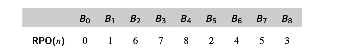
Visiting the nodes in this order produces the sequence of iterations and val- ues shown in Fig. 9.3. Working in RPO, the algorithm computes accurate DOM sets for this graph on the first iteration and halts after the second iter- ation. RPO lets the algorithm halt in two passes over the graph rather than three. Note, however, that the algorithm does not always compute accurate DOM sets in the first pass, as the next example shows.

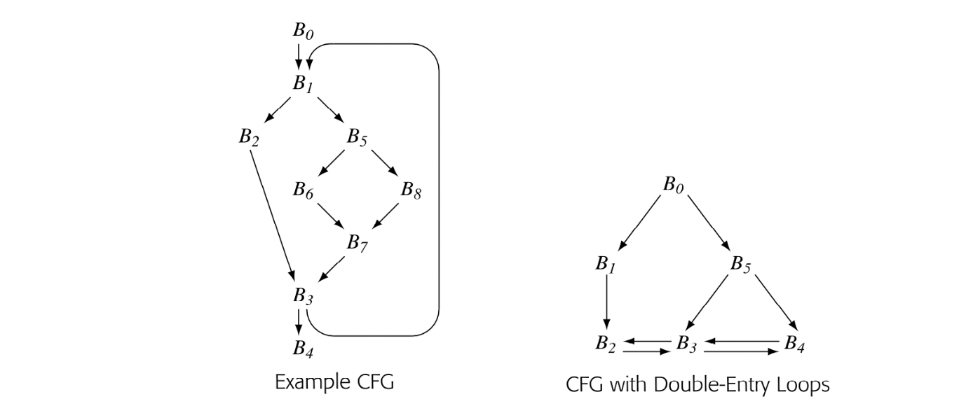
As a second example, consider the second CFG in the margin. It has two loops with multiple entries: $(B_{2}, B_{3})$ and $(B_{3}, B_{4})$ . In particular, $(B_{2}, B_{3})$ has entries from both $(B_{0}, B_{1}, B_{2})$ and $(B_{0}, B_{5}, B_{3})$ , while $(B_{3}, B_{4})$ has entries

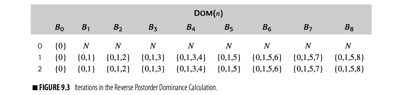
from $(B_{0}, B_{5}, B_{3})$ and $(B_{0}, B_{5}, B_{4})$ . This property makes the graph irreducible, which makes it more difficult to analyze with some data-flow algorithms (see the discussion of reducibility in Section 9.5.1).

To apply the iterative algorithm, we need an rpo numbering. One rpo numbering for this CFG is: Working in this order, the algorithm produces the following iterations:

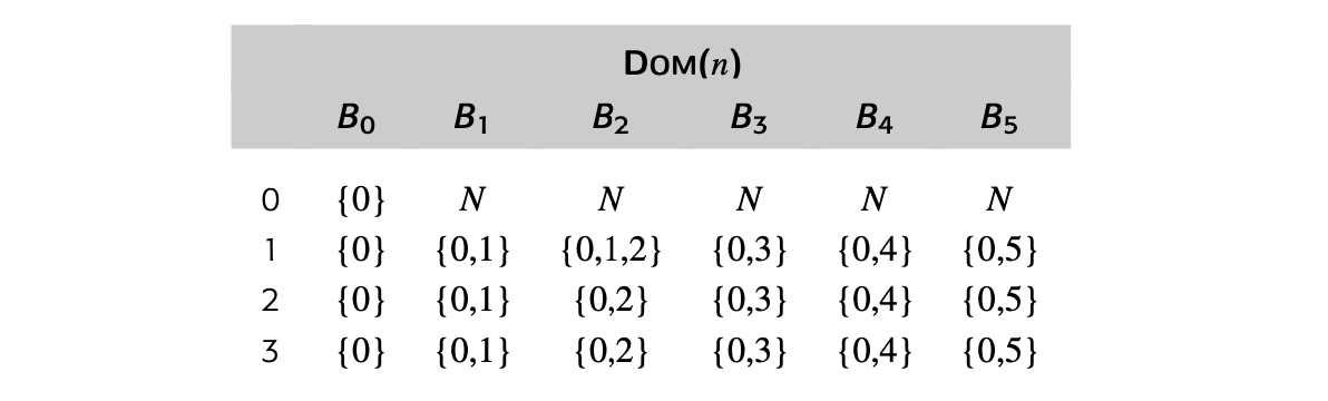
The algorithm requires two iterations to compute the correct DOM sets. The final iteration recognizes that it has reached a fixed point.

The dominance calculation relies only on the structure of the graph. It ig- nores the behavior of the code in any of the CFG’s blocks. As such, it might be considered a form of control-flow analysis. Most data-flow problems in- volve reasoning about the behavior of the code and the flow of data between operations. As an example of this kind of calculation, we will revisit the analysis of live variables.

9.2.2 Live-VariableAnalysis

NAMING SETS IN DATA-FLOW EQUATIONS

In writing the data-flow equations for classic problems, we have renamed the sets that contain local information. The original papers use more intuitive set names. Unfortunately, those names clash with each other across problems. For example, available expressions, live variables, reaching definitions, and anticipable expressions all use some notion of a kill set. These four problems, however, are defined over three distinct domains: expressions (AVAILOUT and ANTOUT), definition points (REACHES), and variables (LIVEOUT). Thus, using one set name, such as KILL or KILLED, can produce confusion across problems.

The names that we have adopted encode both the domain and a hint as to the set’s meaning. Thus, VARKILL(n) contains the set of variables killed in block n, while EXPRKILL(n) contains the set of expressions killed in the same block. Similarly, UEVAR(n) is the set of upward-exposed variables in n, while UEEXPR(n) is the set of upward-exposed expressions. While these names are somewhat awkward, they make explicit the distinction between the notion of kill used in available expressions (EXPRKILL) and the one used in reaching definitions (DEFKILL).

In Section 8.6.1, we used the results of live analysis to identify uninitialized variables. Compilers use live information for many other purposes, such as register allocation and construction of some variants of SSA form. We formulated live analysis as a global data-flow problem with the equation:

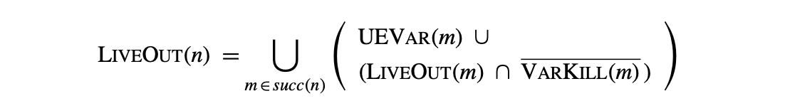
where, succ(n) refers to the set of CFG successors of $n$ . The analysis should initialize $LiveOut (n) = \emptyset, \forall n$ .

Comparing the equations for LiveOut and Dom reveals differences between the problems.

LiveOut is a backward data-flow problem; $LiveOut (n)$ is a function of the information known on entry to each of $n$ 's CFG successors. By contrast, Dom is a forward data-flow problem.
LiveOut looks for a future use on any path in the CFG; thus, it combines information from multiple paths with the union operator. Dom looks for predecessors that lie on all paths from the entry node; thus, it combines information from multiple paths with the intersection operator.
LiveOut reasons about the effects of operations. The sets $UEVAR (n)$ and $VarKill (n)$ encode the effects of executing the block associated with $n$ . By contrast, the Dom equations only use node names. LiveOut uses more information and takes more space.

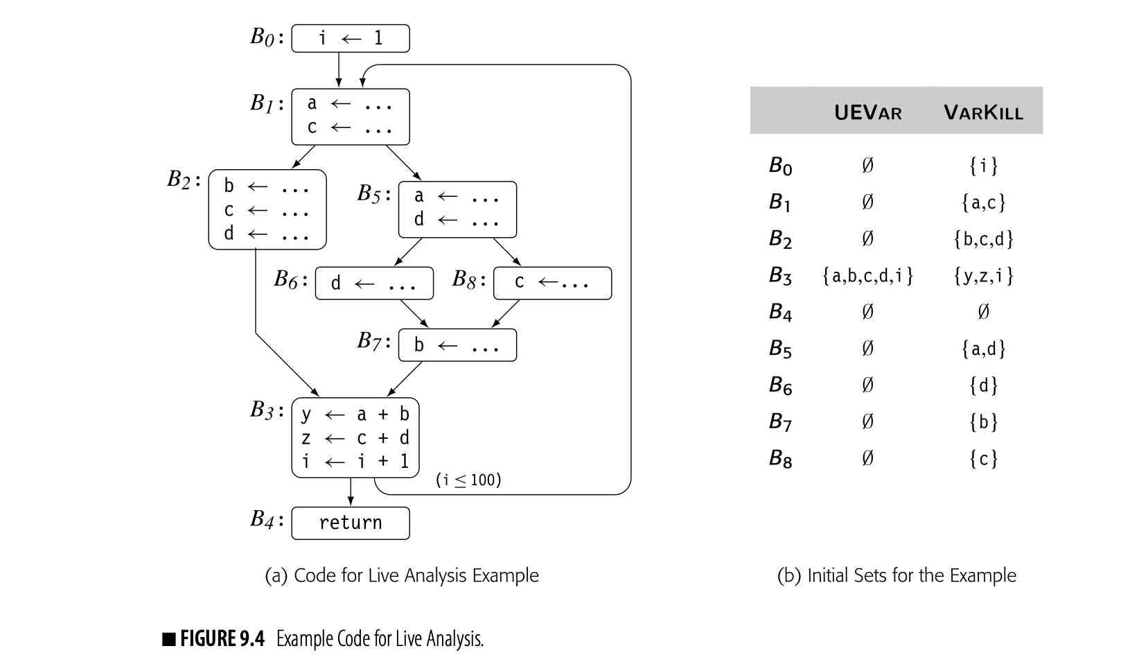
Despite the differences, the process for solving an instance of LiveOut is the same as for an instance of Dom. The compiler must: (1) build a CFG; (2) compute initial values for the sets (see Fig. 8.15(a) on page 420), and (3) apply the iterative algorithm (see Fig. 8.15(b)). These steps are analogous to those taken to solve the Dom equations.

To see the issues that arise in solving an instance of LiveOut, consider the code shown in Fig. 9.4(a). It fleshes out the example CFG that we have used throughout this chapter. Panel (b) shows the UEVar and VarKill sets for each block.

Fig. 9.5 shows the progress of the iterative solver on the example from Fig. 9.4(a), using the same RPO that we used in the Dom computation. Although the equations for LiveOut are more complex than those for Dom, the arguments for termination, correctness, and efficiency are similar to those for the dominance equations.

Termination

Recall that in DOM the sets shrink monoton- ically.

Iterative live analysis halts because the sets grow monotonically and the sets have a finite maximum size. Each time that the algorithm evaluates the LiveOut equation at a node in the cfg, that LiveOut set either remains the same or it grows larger. The LiveOut sets do not shrink. When the algorithm reaches a state where no LiveOut set changes, it halts. It has reached a fixed point.

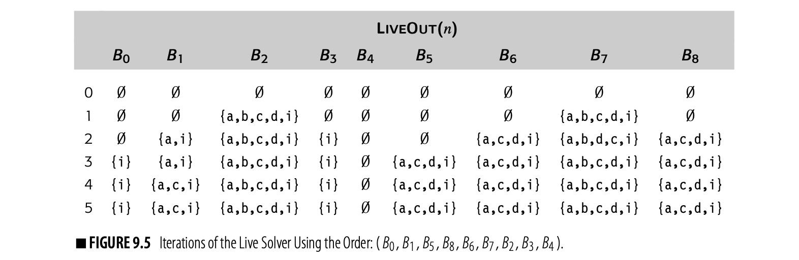The LiveOut sets are finite. Each LiveOut set is either $V$ , the set of names being analyzed, or it is a proper subset of $V$ . In the worst case, one LiveOut set would grow by a single name in each iteration; that behavior would halt after $n \cdot ∣ V ∣$ iterations, where $n$ is the number of nodes in the cfg.

This property-the combination of monotonicity and finite sets-guarantees termination. It is often called the finite descending chain property. In Dom, the sets shrink monotonically and their size is less than or equal to the number of nodes in the cfg. In LiveOut, the sets grow monotonically and their size is bounded by the number of names being analyzed. Either way, it guarantees termination.

Correctness

Iterative live analysis is correct if and only if it finds all the variables that satisfy the definition of liveness at the end of each block. Recall the definition: A variable $v$ is live at point $p$ if and only if there is a path from $p$ to a use of $v$ along which $v$ is not redefined. Thus, liveness is defined in terms of paths in the cfg. A path that contains no definitions of $v$ must exist from $p$ to a use of $v$ . We call such a path a $v$ -clear path.

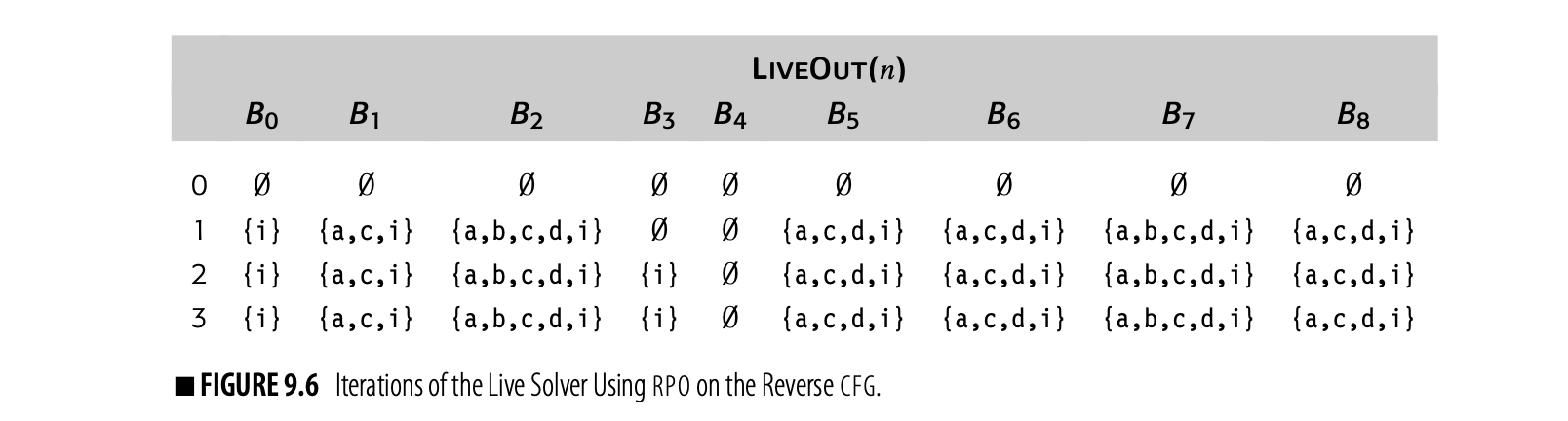
$LiveOut (n)$ should contain $v$ if and only if $v$ is live at the end of block $n$ . To form $LiveOut (n)$ , the iterative solver computes the contribution to $LiveOut (n)$ of each successor of $n$ in the cfg. The contribution of some successor $m$ to $LiveOut (n)$ is given by the right-hand side of the $LiveOut$ equation: $UEVar (m)$ $\cup$ ( $LiveOut (m) \cap \overline{VarKill (m)}$ ).

The solver combines the contributions of the various successors with union because $v \in LiveOut (n)$ if $v$ is live on any path that leaves $n$ .

How does this local computation over single edges relate to liveness defined over all paths? The LiveOut sets that the solver computes are a fixed-point solution to the live equations. Again, the theory of iterative data-flow analysis assures us that the live equations have a unique fixed-point solution [221]. Uniqueness guarantees that all the fixed-point solutions are identical, which includes the meet-over-all-paths solution implied by the definition.

Efficiency

It is tempting to think that reverse postorder on the reverse CFG is equivalent to reverse preorder on the CFG. Exercise 3.b shows a counter-example.

For a backward problem, the solver should use an rpo traversal on the reverse cfg. The iterative evaluation shown in Fig. 9.5 used rpo on the cfg. For the example cfg, one rpo on the reverse cfg is:

Visiting the nodes in this order produces the iterations shown in Fig. 9.6. Now, the algorithm halts in three iterations, rather than the five iterations required with a traversal ordered by rpo on the cfg. Comparing this table against the earlier computation, we can see why. On the first iteration, the algorithm computed correct LiveOut sets for all nodes except $B_{3}$ . It took a second iteration for $B_{3}$ because of the back edge--the edge from $B_{3}$ to $B_{1}$ . The third iteration is needed to recognize that the algorithm has reached its fixed point. Since the fixed point is unique, the compiler can use this more efficient order.

This pattern holds across many data-flow problems. The first iteration computes sets that are correct, except for the effects of cycles. Subsequent iterations settle out the information from cycles.

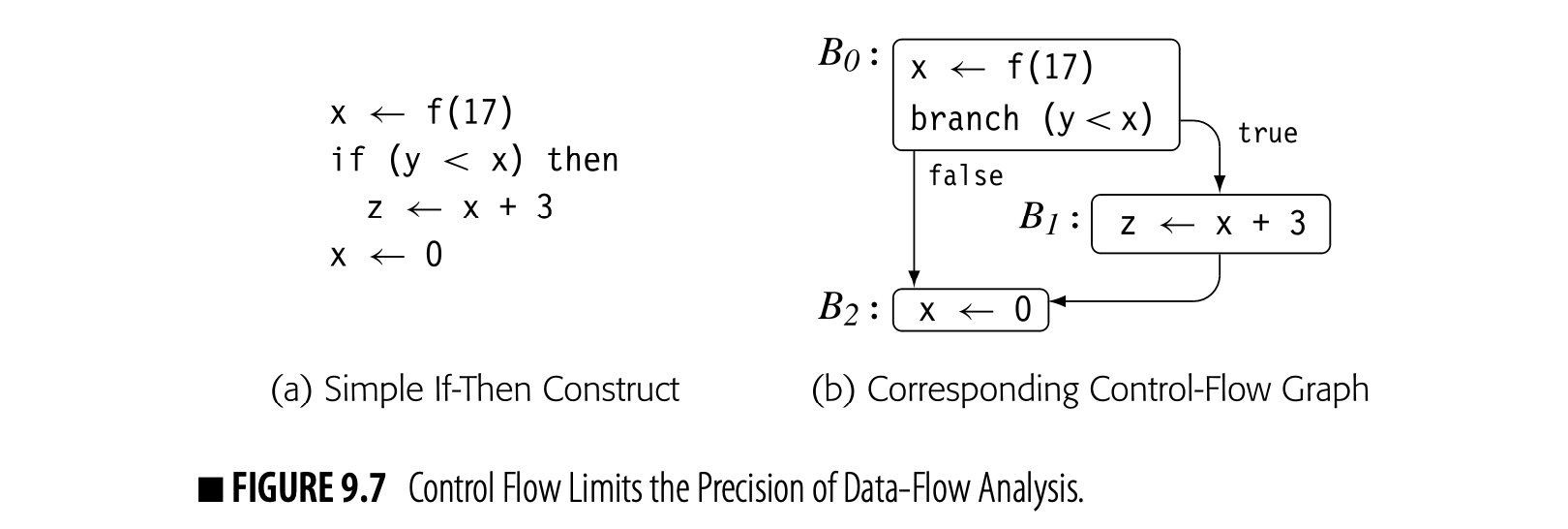
9.2.3 Limitations on Data-Flow Analysis

There are limits to what a compiler can learn from data-flow analysis. In some cases, the limits arise from the assumptions underlying the analysis. In other cases, the limits arise from features of the language being analyzed. To make informed decisions, the compiler writer must understand what data-flow analysis can do and what it cannot do.

When it computes $LiveOut (n)$ , the iterative algorithm uses the sets $LiveOut$ , $UEVar$ , and $VarKill$ for each of $n$ 's CFG successors. This action implicitly assumes that execution can reach each of those successors; in practice, one or more of them may not be reachable.

Consider the code fragment shown in Fig. 9.7 along with its CFG. The definition of x in $B_{O}$ is live on exit from $B_{O}$ because of the use of x in $B_{I}$ . The definition of x in $B_{2}$ kills the value set in $B_{O}$ . If $B_{I}$ cannot execute, then x's value from $B_{O}$ is not live past the comparison with y, and x # $LiveOut (B_{O})$ . If the compiler can prove that the y is always less than x, then $B_{I}$ never executes. The compiler can eliminate $B_{I}$ and replace the test and branch in $B_{O}$ with a jump to $B_{2}$ . At that point, if the call to f has no side effects, the compiler can also eliminate $B_{O}$ .

The equations for $LiveOut$ , however, take the union over all successors of a block, not just its executable successors. Thus, the analyzer computes:

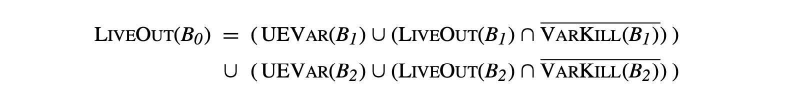
Data-flow analysis assumes that all paths through the CFG are feasible. Thus, the information that they compute summarizes the possible data-flow events, assuming that each path can be taken. This limits the precision of the resulting information; we say that the information is precise "up to symbolic execution." With this assumption, x $\in LiveOut (B_{O})$ and both $B_{O}$ and $B_{I}$ must be preserved.

STATIC ANALYSIS VERSUS DYNAMIC ANALYSIS

The notion of static analysis leads directly to the question: What about dynamic analysis? By definition, static analysis tries to estimate, at compile time, what will happen at runtime. In many situations, the compiler cannot tell what will happen, even though the answer might be obvious with knowledge of one or more runtime values.

Consider, for example, the C fragment:

It contains a redundant expression, $y * z$ , if and only if p does not contain the address of either y or z. At compile time, the value of p and the address of y and z may be unknown. At runtime, they are known and can be tested. Testing these values at runtime would allow the code to avoid recomputing $y * z$ , where compile-time analysis might be unable to answer the question.

However, the cost of testing whether $p == & y$ , or $p == & z$ , or neither and acting on the result is likely to exceed the cost of recomputing y * z. For dynamic analysis to make sense, it must be a priori profitable—that is, the savings must exceed the cost of the analysis. This happens in some cases; in most cases, it does not. By contrast, the cost of static analysis can be amortized over multiple executions of the code, so it is more attractive, in general.

Another way that imprecision creeps into the results of data-flow analysis comes from the treatment of arrays, pointers, and procedure calls. An array reference, such as A[i,j], refers to a single element of A. However, without analysis that reveals the values of i and j, the compiler cannot tell which element of A is accessed. For this reason, compilers have traditionally treated a reference to an element of A as a reference to all of A. Thus, a use of A[i,j] counts as a use of A, and a definition of A[m,n] counts as a definition of A.

The compiler writer must not, however, make too strong an inference. Because the information on arrays is imprecise, the compiler must interpret that information conservatively. Thus, if the goal of the analysis is to determine where a value is no longer live--that is, the value must have been killed--then a definition of A[i,j] does not kill the value of A. If the goal is to recognize where a value might not survive, then a definition of A[i,j] might define any element of A.

Points-to analysis, used to track possible pointer values, is more expensive than classic data-flow problems such as DOM and LIVE.

Pointers add another level of imprecision to the results of static analysis. Explicit arithmetic on pointers makes matters worse. Unless the compiler employs an analysis that tracks the values of pointers, it must interpret an assignment to a pointer-based variable as a potential definition for every variable that the pointer might reach. Type safety can limit the set of objects that the pointer can define; a pointer declared to point at an object of type $t$ can only be used to modify objects of type $t$ . Without analysis of pointer values or a guarantee of type safety, assignment to a pointer-based variable can force the analyzer to assume that every variable has been modified. In practice, this effect often prevents the compiler from keeping the value of a pointer-based variable in a register across any pointer-based assignment. Unless the compiler can specifically prove that the pointer used in the assignment cannot refer to the memory location corresponding to the enregistered value, it cannot safely keep the value in a register.

The complexity of analyzing pointer use leads many compilers to avoid keeping values in registers if they can be the target of a pointer. Usually, some variables can be exempted from this treatment--such as a local variable whose address has never been explicitly taken. The alternative is to perform data-flow analysis aimed at disambiguating pointer-based references--reducing the set of possible variables that a pointer might reference at each point in the code. If the program can pass pointers as parameters or use them as global variables, pointer disambiguation becomes inherently interprocedural.

Procedure calls provide a final source of imprecision. To understand the data flow in the current procedure, the compiler must know what the callee can do to each variable that is accessible to both the caller and the callee. The callee may, in turn, call other procedures that have their own potential side effects.

Unless the compiler computes accurate summary information for each procedure call, it must estimate the call's worst-case behavior. While the specific assumptions vary across problems and languages, the general rule is to assume that the callee both uses and modifies every variable that it can reach. Since few procedures modify and use every variable, this rule typically overestimates the impact of a call, which introduces further imprecision into the results of the analysis.

9.2.4 Other Data-Flow Problems

Compilers use data-flow analyses to prove the safety of applying transformations in specific situations. Thus, many distinct data-flow problems have been proposed, each for a particular optimization.

Availability

Availability An expression $e$ is available at point $p$ if and only if, on every path from the procedure's entry to $p$ , $e$ is evaluated and none of its operands is redefined.

To identify redundant expressions, the compiler can compute information about the availability of expressions. This analysis annotates each node $n$ in the CFG with a set $AvailIn (n)$ , which contains the names of all expressions in the procedure that are available on entry to the block corresponding to $n$ . The equations for $AvailIn$ are:

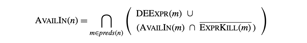with initial values for the $AvailIn$ sets:

These equations can be solved efficiently with a standard iterative data-flow solver. Since it is a forward data-flow problem, the solver should use RPO on the CFG.

In the equations, $DEExpr (n)$ is the set of downward-exposed expressions in $n$ . An expression $e \in DEExpr (n)$ if and only if block $n$ evaluates $e$ and none of $e$ 's operands is defined between the last evaluation of $e$ in $n$ and the end of $n$ . $ExprKill (n)$ contains all those expressions that are killed by a definition in $n$ . An expression is killed if one or more of its operands are redefined in the block.

An expression $e$ is available on entry to $n$ if and only if it is available on exit from each of $n$ 's predecessors in the CFG. As the equation states, an expression $e$ is available on exit from some block $m$ if one of two conditions holds: either $e$ is downward exposed in $m$ , or it is available on entry to $m$ and is not killed in $m$ .

AvailIn sets are used in global redundancy elimination, sometimes called global common subexpression elimination. Perhaps the simplest way to achieve this effect is to compute $AvailIn$ sets for each block and use them as initial information in local value numbering (see Section 46.1). Lazy code motion is a stronger form of redundancy elimination that also uses availability (see Section 46.1).

Reaching Definitions

In some cases, the compiler needs to know where an operand was defined. If multiple paths in the CFG lead to the operation, then multiple definitions may provide the value of the operand. To find the set of definitions that reacha block, the compiler can compute reaching definitions. The compiler annotates each node $n$ in the CFG with a set, $Reaches (n)$ that contains the name of every definition that reaches the head of the block corresponding to $n$ . The domain of $Reaches$ is the set of definition points in the procedure--the set of assignments.

The compiler computes a set $Reaches (n)$ for each CFG node $n$ using the equation:

with initial values for the Reaches sets: $DEDef (m)$ is the set of downward-exposed definitions in $m$ : those definitions in $m$ for which the defined name is not subsequently redefined in $m$ . $DefKill (m)$ contains all the definition points that are obscured by a definition of the same name in $m$ ; $d \in DefKill (m)$ if $d$ defines some name $v$ and $m$ contains a definition that also defines $v$ . Thus, $\overline{DefKill (m)}$ contains those definition points that survive through $m$ .

$DEDef$ and $DefKill$ are both defined over the set of definition points, but computing each of them requires a mapping from names (variables and compiler-generated temporaries) to definition points. Thus, gathering the initial information for reaching definitions is more expensive than it is for live variables.

Anticipable Expressions

Anticipability An expression, $e$ , is anticipable at point $p$ if and only if (1) every path that leaves $p$ evaluates $e$ , and (2) evaluating $e$ at $p$ would produce the same result as the first evaluation along each of those paths.

In some situations, the compiler can move an expression backward in the CFG and replace multiple instances of the $e x p ress i o n$ , along different paths, with a single instance. This optimization, called hoisting, reduces code size. It does not change the number of times the expression is evaluated.

To find safe opportunities for hoisting, the compiler can compute the set of anticipable expressions at the end of each block. An expression $e$ is anticipable at the end of block $b$ if the next evaluation of $e$ , along each path leaving $b$ , would produce the same result. The equations require that $e$ be computed along every path that leaves $b$ .

$AntOut$ , the set of expressions anticipable at the end of a block, can be computed as a backward data-flow problem on the CFG. Anticipability is formulated over the domain of expressions.

Implementing Data-Flow Frameworks

The equations for many global data-flow problems show a striking similarity. For example, available expressions, live variables, reaching definitions, and anticipable expressions all have propagation functions of the form: where $c_{1}$ and $c_{2}$ are constants derived from the code and $o p_{1}$ and $o p_{2}$ are standard set operations such as $\cup$ and $\cap$ . This similarity appears in the problem descriptions; it creates the opportunity for code sharing in the implementation of the analyzer.

The compiler writer can easily abstract away the details in which these problems differ and implement a single, parameterized analyzer. The analyzer needs functions to compute $c_{1}$ and $c_{2}$ , implementations of the operators, and an indication of the problem's direction. In return, it produces the desired data-flow sets.

This implementation strategy encourages code reuse. It hides the low-level details of the solver. It also creates a situation in which the compiler writer can profitably invest effort in optimizing the implementation. For example, a scheme that implements $f (x) = c_{1} o p_{1} (x o p_{2} c_{2})$ as a single function may outperform one that implements both $f_{1} (x) = c_{1} o p_{1} x$ and $f_{2} (x) = x o p_{2} c_{2}$ , and computes $f (x)$ as $f_{1} (f_{2} (x))$ . A framework lets all the client transformations benefit from improvements in the set representations and operator implementations.

The equations to define AntOut are:

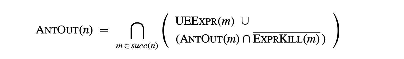
with initial values for the AntOut sets:

Here $U EEXPR (m)$ is the set of upward-exposed expressions—those used in $m$ before they are killed. $EXPR K I LL (m)$ contains all those expressions that are killed by a definition in $m$ ; it also appears in the equations for available expressions.

The results of anticipability analysis are used in lazy code motion, to de- crease execution time, and in code hoisting, to shrink the size of the compiled code. Both transformations are discussed in Section 10.3.

Interprocedural Summary Problems

When analyzing a single procedure, the compiler must account for the impact of each procedure call. In the absence of specific information about the call, the compiler must make worst-case assumptions about the callee and about any procedures that it, in turn, calls. These assumptions can seriously degrade the precision of the global data-flow information. For example, the compiler must assume that the callee modifies every variable that it can access; this assumption essentially stops the propagation of facts across a call site for all global variables, module-level variables, and call-by-reference parameters.

To limit such impact, the compiler can compute summary information on each call site. The classic summary problems compute the set of variables that might be modified as a result of the call and that might be used as a result of the call. The compiler can then use these computed summary sets in place of its worst case assumptions.

Flow insensitive This formulation of MAYMOD ignores control flow inside procedures. Such a formulation is said to be flow $in se n s i t i v e$ .

The $in t er p roce d u r a l$ may modify problem_ annotates each call site with a set of names that the callee, and procedures it calls, might modify. May modify is one of the simplest problems in interprocedural analysis, but it can have a significant impact on the quality of information produced by other analyses, such as global constant propagation. May modify is posed as a set of data-flow equations over the program's call graph that annotate each procedure with a MayMod set.

$M A Y MO D (p)$ is initialized to contain all the names modified locally in $p$ that are visible outside $p$ . It is computed as the set of names defined in $p$ minus any names that are strictly local to $p$ .

The function $u nbin d_{e}$ maps one set of names into another. For a call-graph edge $e = (p, q)$ and set of names $s$ , $u nbin d_{e} (s)$ maps each name in s from the name space of $q$ to the name space that holds at the call site, using the bindings at the call site that corresponds to $e$ . In essence, it projects s from $q$ 's name space into p 's name space.

Given a set of $L OC A L MO D$ sets and a call graph, an iterative solver will find a fixed-point solution for these equations. It will not achieve the kind of fast time bound seen in global data-flow analysis. A more complex framework is required to achieve near-linear complexity on this problem (see Chapter Notes).

The MayMod sets computed by these equations are generalized summary sets. That is, MayMod( $q$ ) contains the names of variables that might be modified by a call to $q$ , expressed in the name space of $q$ . To use this information at a specific call site that invokes $q$ , the compiler will compute the set $S = unbind_{e} (MayMod (q))$ , where $e = (p, q)$ is the call graph edge corresponding to the call. The compiler must then add to $S$ any names that are aliased inside $p$ to names contained in $S$ .

The compiler can also compute the set of variables that might be referenced as a result of executing a procedure call, the interprocedural may reference problem. The equations to annotate each procedure $p$ with a set MayRef( $p$ ) are similar to the equations for $M a y M o d$ The function unbind e_{e} maps one set of names into another. For a call-graph edge e=(p, q) and set of names s, unbind d_{e}(s) maps each name in s from the name space of q to the name space that holds at the call site, using the bindings at the call site that corresponds to e. In essence, it projects s from q 's name space into p 's name space.\\Given a set of LOCALMOD sets and a call graph, an iterative solver will find a fixed-point solution for these equations. It will not achieve the kind of fast time bound seen in global data-flow analysis. A more complex framework is required to achieve near-linear complexity on this problem (see Chapter Notes)..

Section Review

Iterative data-flow analysis works by repeatedly reevaluating an equation at each node in some underlying graph until the sets defined by the equations reach a fixed point. Many data-flow problems have a unique fixed point, which ensures a correct solution independent of the evaluation order, and the finite descending chain property, which guarantees termination independent of the evaluation order. These two properties allow the compiler writer to choose evaluation orders that converge quickly. As a result, iterative analysis is robust and efficient.

The literature describes many different data-flow problems. Examples in this section include dominance, live analysis, availability, anticipability, and interprocedural summary problems. All of these, save for the interprocedural problems, have straightforward efficient solutions with the iterative algorithm. To avoid solving multiple problems, compilers often turn to a unifying framework, such as SSA form, described in the next section.

Review Questions

Compute Dom sets for the CFG shown in the margin, evaluating the nodes in the order $(B_{d}, B_{2}, B_{1}, B_{5}, B_{3}, B_{0})$ . Explain why this order takes a different number of iterations than is shown on page 456.
When the compiler builds a call graph, ambiguous calls can complicate the process, much as ambiguous jumps complicate CFG construction. What language features might lead to an ambiguous call site--one where the compiler was uncertain of the callee5 identify?

9.3 Static Single-Assignment Form

Over time, compiler writers have formulated many different data-flow problems. If each transformation uses its own analysis, the effort spent implementing, debugging, and maintaining the analysis passes can grow unreasonably large. To limit the number of analyses that the compiler writer must implement and that the compiler must run, it is desirable to use a single analysis for multiple transformations.

Some compilers, such as LLVM/CLANG, use SSA as their definitive IR.

One strategy for such a "universal" analysis is to build an IR called static single-assignment form (ssa) (see also Section 4.6.2). SSA encodes both data flow and control flow directly into the IR. Many of the classic scalar optimizations have been reworked to operate on code in SSA form.

Code in SSA form obeys two rules:

Each computation in the procedure defines a unique name.
Each use in the procedure refers to a single name.

The first rule removes the effect of "kills" from the code; any expression in the code is available at any point after it has been evaluated. (We first saw this effect in local value numbering.) The second rule has a more subtle effect. It ensures that the compiler can still represent the code concisely and correctly; a use can be written with a single name rather than a long list of all the definitions that might reach it. 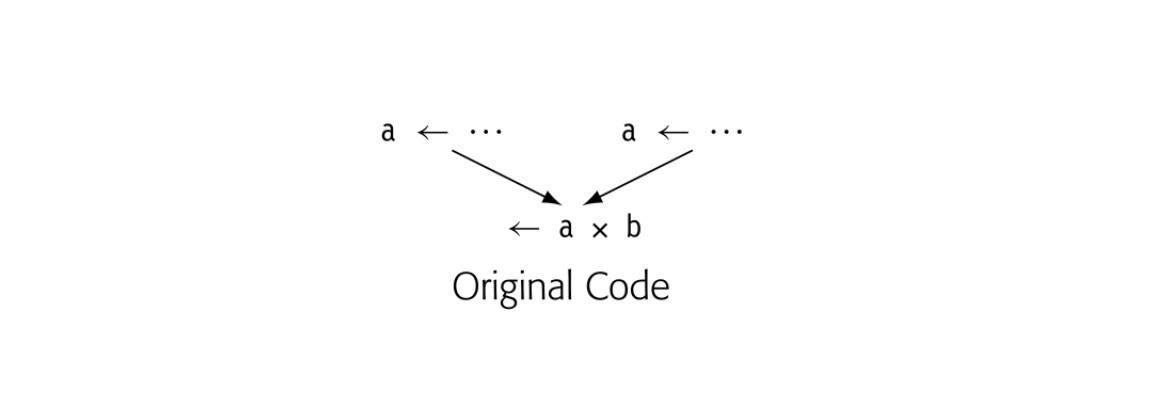Consider the small example shown in the margin. If the compiler renames the two definitions of a to a and, what name should appear in the use of a in a? Neither nor will work in a?b. (The example assumes that was defined earlier in the code.)

To manage this name space, the SSA construction inserts a special kind of copy operation, a $ϕ$ -function, at the head of the block where control-flow paths meet, as shown in the margin. When the $ϕ$ -function evaluates, it reads the argument that corresponds to the edge from which control flow entered the block. Thus, coming from the block on the left, the $ϕ$ -function reads, while from the block on the right it reads. The selected argument is assigned to. Thus, the evaluation of computes the same value that did in the pre-SSA code.

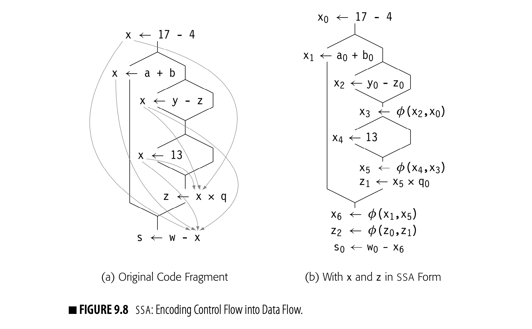Fig. 9.8 shows a more extensive example. Consider the various uses of the variable $x$ in the code fragment shown in panel (a). The curved gray lines show which definitions can reach each use of $x$ . Panel (b) shows the same fragment in SSA form. Variables have been renamed with subscripts to ensure unique names for each definition. We assume that, and are defined earlier in the code.

The code in panel (b) includes all of the $ϕ$ -functions needed to reconcile the names generated by rule one with the need for unique names in uses. Tracing the flow of values will reveal that the same values follow the same paths as in the original code.

Two final points about $ϕ$ -functions need explanation. First, $ϕ$ -functions are defined to execute concurrently. When control enters a block, all of the block's $ϕ$ -functions read their designated argument, in parallel. Next, they all define their target names, in parallel. This concurrent execution semantics allows the SSA construction algorithm to ignore the order of $ϕ$ -functions as it inserts them into a block.

Second, by convention, we write the arguments of a $ϕ$ -function left-to-right to correspond with the incoming edges left-to-right on the printed page. Inside the compiler, the IR has no natural notion of left-to-right for the edges entering a block. Thus, the implementation will require some bookkeeping to track the correspondence between $ϕ$ -function arguments and CFG edges.

9.3.1 A Naive Method for Building SSA Form

Both of the SSA-construction algorithms that we present follow the same basic outline: (1) insert $ϕ$ -functions as needed and (2) rename variables and temporary values to conform with the two rules that define SSA form. The simplest construction method implements the two steps as follows:

The "naive" algorithm inserts more $ϕ$ -functions than are needed. It adds a $ϕ$ - function for each name at each join point.

Inserting $ϕ$ -functions At the start of each block that has multiple CFG predecessors, insert a $ϕ$ -function, such as x $\leftarrow ϕ$ (x,x), for each name x that the current procedure defines. The $ϕ$ -function should have one argument for each predecessor block in the CFG. This process inserts a $ϕ$ -function in every case that might need one. It also inserts many extraneous $ϕ$ -functions.
Renaming The $ϕ$ -function insertion algorithm ensures that a $ϕ$ -function for $x$ is in place at each join point in the CFG reached by two or more definitions of $x$ . The renaming algorithm rewrites all of the names into the appropriate SSA names. The first step adds a unique subscript to the name at each definition.

Base name In an SSA name $x_{2}$ , the base name is x and the version is 2 .

At this point, each definition has a unique SSA name. The compiler can compute reaching definitions (see Section 9.2.4) to determine which SSA name reaches each use. The compiler writer must change the meaning of DefKill so that a definition to one SSA name kills not only that SSA name but also all SSA names with the same base name. The effect is to stop propagation of an SSA name at any $ϕ$ -function where it is an argument. With this change, exactly one definition--one SSA name--reaches each use. The compiler makes a pass over the code to rewrite the name in each use with the SSA name that reaches it. This process rewrites all the uses, including those in $ϕ$ -function arguments. If the same SSA name reaches a $ϕ$ -function along multiple paths, the corresponding $ϕ$ -function arguments will have the same SSA name. The compiler must sort out the correspondence between incoming edges in the CFG and $ϕ$ -function arguments so that it can rename each argument with the correct SSA name. While conceptually simple, this task requires some bookkeeping.

A $ϕ$ -function $x_{j} \leftarrow ϕ (x_{i}, x_{i})$ is redundant. A $ϕ$ -function whose value is not live is considered dead.

The naive algorithm constructs SSA form that obeys the two rules. Each definition assigns to a unique name; each reference uses the name of a distinct definition. While the algorithm builds correct SSA form, it can insert $ϕ$ -functions that are redundant or dead. These extra $ϕ$ -functions may be problematic. The compiler wastes memory representing them and time traversing them. They can also decrease the precision of some kinds of analysis over SSA form.

We call this flavor of SSA maximal SSA form. To build SSA form with fewer $ϕ$ -functions requires more work; in particular, the compiler must analyze the code to determine where potentially distinct values converge in the CFG. This computation relies on the dominance information described in Section 9.2.1.

The difference of SSA form of SSA Form

The literature proposes several distinct flavors of SSA form. The flavors differ in their criteria for inserting $ϕ$ -functions. For a given program, they can produce different sets of $ϕ$ -functions.

Minimal SSA inserts a $ϕ$ -function at any join point where two distinct definitions for the same original name meet. This is the minimal number consistent with the definition of SSA. Some of those $ϕ$ -functions, however, may be dead; the definition says nothing about the values being live when they meet.

Pruned SSA adds a liveness test to the $ϕ$ -insertion algorithm to avoid adding dead $ϕ$ -functions. The construction must compute LwEOUT sets, which increases the cost of building pruned SSA.

Semipruned SSA is a compromise between minimal SSA and pruned SSA. Before inserting $ϕ$ -functions, the algorithm eliminates any names that are not live across a block boundary. This can shrink the name space and reduce the number of $ϕ$ -functions without the overhead of computing LwEOUT sets. The algorithm in Fig. 9.11 computes semipruned SSA.

Of course, the number of $ϕ$ -functions depends on the specific program being converted into SSA form. For some programs, the reductions obtained by semipruned SSA and pruned SSA are significant. Shrinking the SSA form can lead to faster compilation, since passes that use SSA form then operate on programs that contain fewer operations--and fewer $ϕ$ -functions.

The following subsections present, in detail, an algorithm to build semipruned SSA--a version with fewer $ϕ$ -functions. Section 9.3.2 introduces dominance frontiers and shows how to compute them; dominance frontiers guide $ϕ$ -function insertion. Section 9.3.3 gives an algorithm to insert $ϕ$ -functions, and Section 9.3.4 presents an efficient algorithm for renaming. Section 9.3.5 discusses complications that can arise in translating out of SSA form.

9.3.2 Dominance Frontiers

The primary problem with maximal SSA form is that it contains too many $ϕ$ -functions. To reduce their number, the compiler must determine more carefully where they are needed. The key to $ϕ$ -function insertion lies in understanding which names need a $ϕ$ -function at each join point. To solve this problem efficiently and effectively, the compiler can turn the question around. It can determine, for each block $i$ , the set of blocks that will need a $ϕ$ -function as the result of a definition in block $i$ . Dominance plays a critical role in this computation.

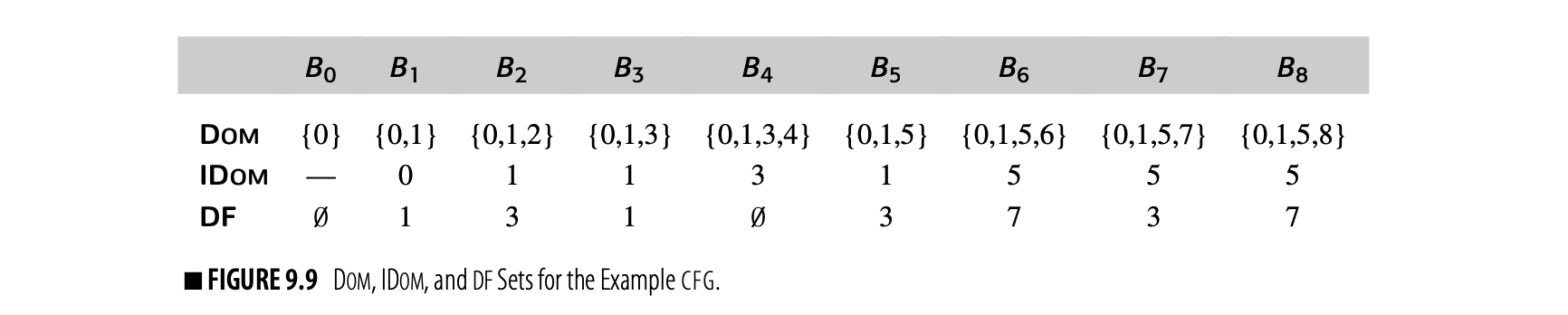
Consider the CFG shown in the margin. Assume that the code assigns distinct values to $a$ in both $B_{I}$ and $B_{5}$ , and that no other block assigns to $a$ . The value from $B_{5}$ is the only value for $a$ that can reach $B_{6}$ , $B_{7}$ , and $B_{8}$ . Because $B_{5}$ dominates these three blocks, it lies on any path from $B_{0}$ to $B_{6}$ , $B_{7}$ , or $B_{8}$ . The definition in $B_{I}$ cannot reach them.

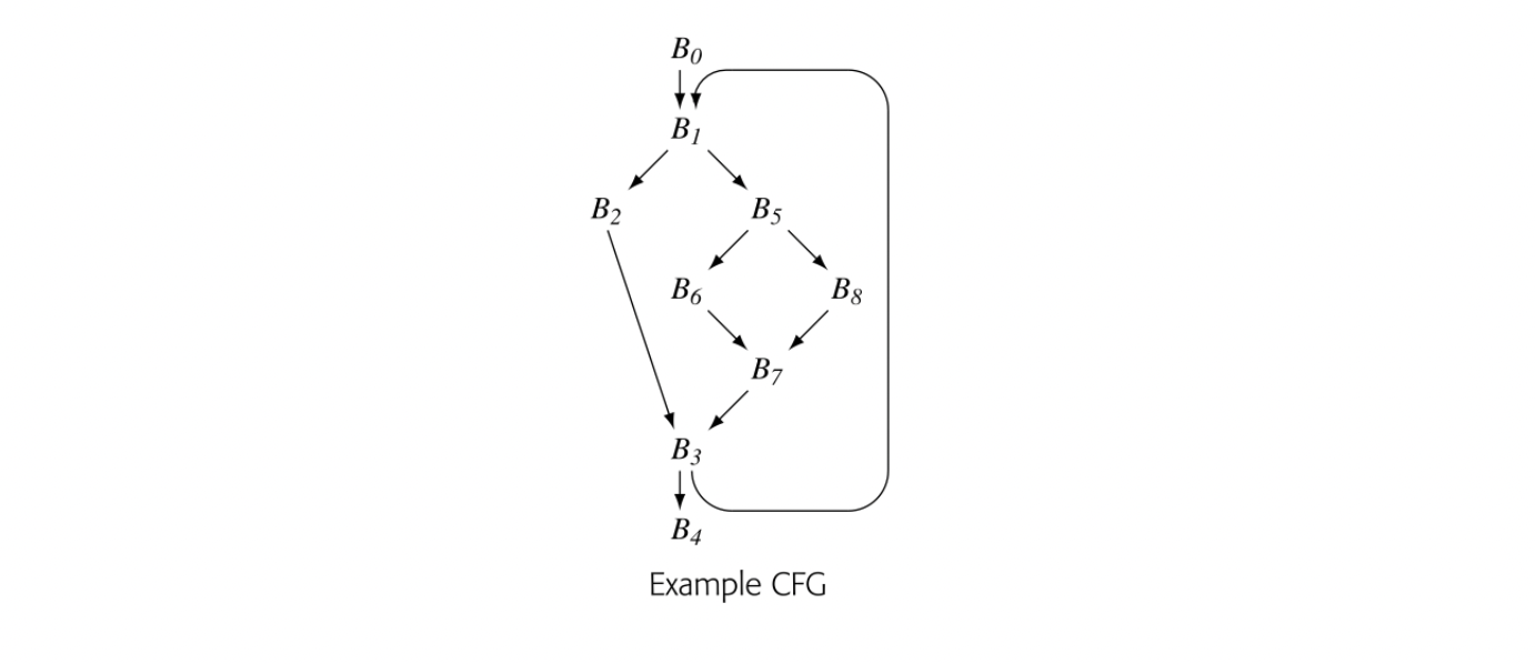
Strict dominance In a CFG, node $p$ strictly dominates node $q$ if $p \in Dom (q)$ and $p \neq = q$ . We denote this as $p \in (Dom (q) - q)$ .

$B_{3}$ presents a different situation. Neither of its CFG predecessors, $B_{2}$ and $B_{7}$ , dominate $B_{3}$ . A use of $a$ in $B_{3}$ can receive its value from either $B_{I}$ or $B_{5}$ , depending on the path taken to reach $B_{3}$ . The assignments to $a$ in $B_{I}$ and $B_{5}$ force a $ϕ$ -function for $a$ at the start of $B_{3}$ .

$B_{5}$ dominates the region $(B_{6}, B_{7}, B_{8})$ . It is the immediate dominator of all three nodes. A definition of $a$ in $B_{5}$ will reach a use in that region, unless $a$ is redefined before the use. The definition in $B_{5}$ cannot necessitate the need for a $ϕ$ -function in this region.

Strict dominance In a CFG, node p strictly dominates node q if $p \in Dom (q)$ and $p \neq = q$ . We denote this as $p \in (Dom (q) - q)$ .

$B_{3}$ lies just outside of the region that $B_{5}$ dominates. It has two CFG predecessors and $B_{5}$ only dominates one of them. Thus, it lies one CFG edge outside the region that $B_{5}$ dominates. In general, a definition of $a$ in some block $B_{i}$ will necessitate a $ϕ$ -function in any node that, like $B_{3}$ , lies one CFG edge beyond the region that $B_{i}$ dominates. The dominance frontier of $B_{i}$ , denoted DF( $B_{i}$ ), is the set of all such nodes.

Dominance frontier In a CFG, node $q$ is in the dominance frontier of node p if and only if (1) p dominates a CFG predecessor of $q$ and (2) p does not strictly dominate $q$ . We denote p 's dominance frontier as $DF (p)$ .

To recap, $q \in$ DF( $p$ ) if, along some path, $q$ is one edge beyond the region that $p$ dominates. Thus:

$q$ has a CFG predecessor that $p$ dominates. There exists an $x$ such that $(x, q)$ is a CFG edge and $p \in Dom (x)$ .
$p$ does not strictly dominate $q$ . That is, $p \in / (Dom (q) - q)$ .

DF( $p$ ) is simply the set of all nodes that meet these two criteria.

A definition of $a$ in block $n$ forces the insertion of a $ϕ$ -function for $a$ at the head of each block $m \in$ DF( $n$ ). Fig. 9 shows the Dom, IDom, and DF sets for the example CFG.

Notice the role of strict dominance. In the example CFG, strict dominance ensures that $B_{1} \in$ DF( $B_{1}$ ). Thus, an assignment to some name $a$ in $B_{1}$ forces

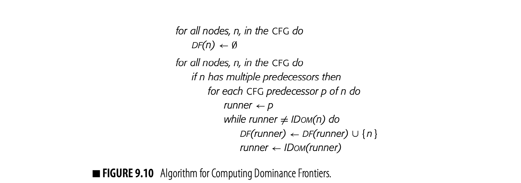
the insertion of a $ϕ$ -function in $B_{1}$ . If the definition of dominance frontiers used Dom, instead, $DF (B_{1})$ would be empty.

Dominator Trees

Dominator tree a tree that encodes the dominance informa- tion for a flow graph

The algorithm to compute dominance frontiers uses a data structure, the dominator tree, to encode dominance relationships. The dominator tree of a CFG has a node for each block in the CFG. Edges encode immediate dominance; if $m = IDom (n)$ , then $n$ is a child of $m$ in the dominator tree.

The dominator tree encodes the Dom sets as well. For a node $n$ , $Dom (n)$ contains precisely the nodes on the path from $n$ to the root of the dominator tree. The nodes on that path are ordered by the IDom relationship. The dominator tree for our running example appears in the margin.

Computing Dominance Frontiers

To make $ϕ$ -insertion efficient, the compiler should precompute, for each CFG node $n$ , a set $DF (n)$ that contains $n$ 's dominance frontier. The algorithm, shown in Fig. 9.10, uses both the dominator tree and the CFG to build the $DF (n)$ sets.

Notice that the DF sets can only contain nodes that are join points in the CFG--that is, nodes that have multiple predecessors. Thus, the algorithm starts with the join points. At a CFG join point $n$ , it iterates over $n$ 's CFG predecessors $p$ and inserts $n$ into $DF (p)$ as needed.

If $p = IDom (n)$ , then p also dominates all of n 's other predecessors. In the example, $B_{0} = IDom (B_{1})$ .

If $p = IDom (n)$ , then $n$ does not belong to $DF (p)$ . Neither does it belong to $DF (m)$ for any predecessor $m$ of $p$ .
If $p \neq = IDom (n)$ , then $n$ belongs in $DF (p)$ . It also belongs in $DF (q)$ for any $q$ such that $q \in Dom (p)$ and $q \in / (Dom (n) - n)$ . The algorithm finds these latter nodes $q$ by running up the dominator tree.

The algorithm follows from these observations. It initializes $DF (n)$ to $\emptyset$ , for all CFG nodes $n$ . Next, it finds each CFG join point $n$ and iterates over $n$ 's

CFG predecessors, $p$ . If $p$ dominates $n$ , the algorithm is done with $p$ . If not, it adds $n$ to DF( $p$ ) and walks up the dominator tree, adding $n$ to the DF set of each dominator-tree ancestor until it finds $n$ 's immediate dominator. The algorithm needs a small amount of bookkeeping to avoid adding $n$ to a DF set multiple times. 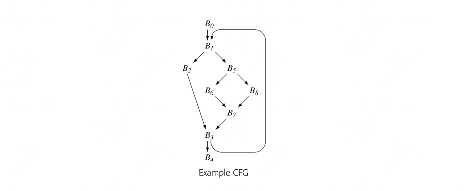Consider again the example CFG and its dominator tree. The analyzer examines the nodes in some order, looking for nodes with multiple predecessors. Assuming that it takes the nodes in name order, it finds the join points as $B_{1}$ , then $B_{3}$ , then $B_{7}$ .

For CFG-predecessor $B_{0}$ , the algorithm finds that $B_{0}$ is IDom( $B_{1}$ ), so it never enters the while loop. For CFG-predecessor $B_{3}$ , it adds $B_{1}$ to DF( $B_{3}$ ) and sets $r u nn er$ to IDom( $B_{3}$ ) = $B_{1}$ . It adds $B_{1}$ to DF( $B_{1}$ ) and sets $r u nn er$ to IDom( $B_{1}$ ) = $B_{0}$ , where it halts.
For CFG-predecessor $B_{2}$ , it adds $B_{3}$ to DF( $B_{2}$ ) and sets $r u nn er$ to IDom( $B_{2}$ ) = $B_{1}$ . Since $B_{1}$ = IDom( $B_{3}$ ), it halts. For CFG-predecessor $B_{7}$ , it adds $B_{3}$ to DF( $B_{7}$ ) and sets $r u nn er$ to IDom( $B_{7}$ ) = $B_{5}$ . It adds $B_{3}$ to DF( $B_{5}$ ) and sets $r u nn er$ to IDom( $B_{5}$ ) = $B_{1}$ , where it halts.
For CFG-predecessor $B_{6}$ , it adds $B_{7}$ to DF( $B_{6}$ ) and advances $r u nn er$ to IDom( $B_{6}$ ) = $B_{5}$ , where it halts. For CFG-predecessor $B_{8}$ , it adds $B_{7}$ to DF( $B_{8}$ ) and advances $r u nn er$ to IDom( $B_{8}$ ) = $B_{5}$ , where it halts.

These results produce the DF sets shown in the table in Fig. 9.9.

9.3.3 Placing $ϕ$ -Functions

The naive algorithm placed a $ϕ$ -function for every variable at the start of every join node. With dominance frontiers, the compiler can determine more precisely where $ϕ$ -functions might be needed. The basic idea is simple.

From a control-flow perspective, an assignment to $x$ in CFG node $n$ induces a $ϕ$ -function in every CFG node m\in\mbox{DF}(n). Each inserted $ϕ$ -function creates a new assignment; that assignment may, in turn, induce additional $ϕ$ -functions.
From a data-flow perspective, a $ϕ$ -function is only necessary if its result is live at the point of insertion. The compiler could compute live information and check each $ϕ$ -function on insertion; that approach leads to pruned SSA form.

The word $g l o ba l$ is used here to mean of interest across the entire procedure.

In practice, the compiler can avoid most dead $ϕ$ -functions with an inexpensive approximation to liveness. A name $x$ cannot need a $ϕ$ -function unless it is live in multiple blocks. The compiler can compute the set of global names--those that are live in multiple blocks. The SSA-construction can ignore any nonglobal name, which reduces the name space and the number of $ϕ$ -functions. The resulting SSA form is called $semipruned SSA form$ .

The compiler can find the global names cheaply. In each block, it looks for names with upward-exposed uses--the UEVar set from the live-variables calculation. Any name that appears in a LiveOut set must be in the UEVar set of some block. Taking the union of all the UEVar sets gives the compiler the set of names that are live on entry to one or more blocks and, hence, live in multiple blocks.

The algorithm to find global names, shown in Fig. 11(a), is derived from the obvious algorithm for computing UEVar. It constructs both a set of global names, Globals, and, for each name, the set of blocks that contain a definition of that name. The algorithm uses these block lists to form initial worklists during $ϕ$ -function insertion.

The algorithm for inserting $ϕ$ -functions, in panel (b), iterates over the global names. For each name $x$ , it initializes WorkList with Blocks( $ϕ$ ). For each block $b$ in WorkList, it inserts a $ϕ$ -function at the head of each block $d$ in $b$ 's dominance frontier. The parallel execution semantics of the $ϕ$ -functions lets the algorithm insert them at the head of $d$ in any order. When it adds a $ϕ$ -function for $x$ to $d$ , the algorithm adds $d$ to WorkList to reflect the new assignment to $x$ in $d$ .

Example

Fig. 9.12 recaps our running example. Panel (a) shows the code and panel (b) shows the dominance frontiers for the CFG.

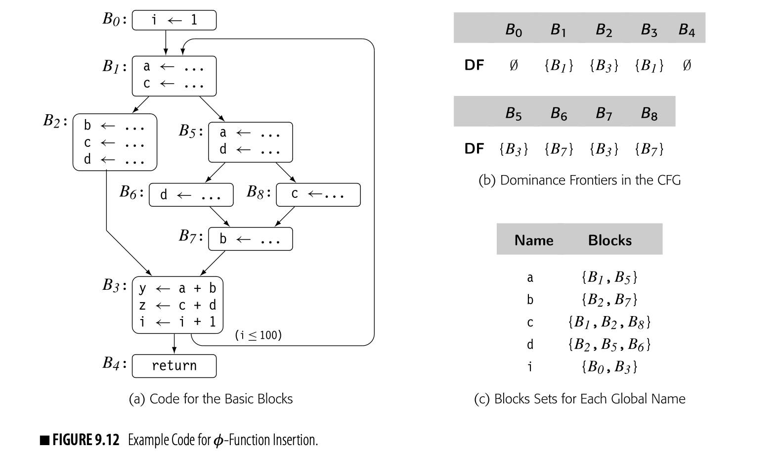
The compiler could avoid computing Blocks sets for nonglobal names, at the cost of another pass over the code.

The first step in the $ϕ$ -function insertion algorithm finds global names and computes the $Blocks$ set for each name. The global names are ${a, b, c, d, i}$ . The $Blocks$ sets for the global names are shown in panel (c). While the algorithm computes a $Blocks$ set for each of y and z, the table omits them because they are not global names.

The $ϕ$ -function insertion algorithm, shown in Fig. 9.11(b), works on a name-by-name basis. Consider its actions for the variable a in the example. First, it initializes the worklist to $Blocks (a) = {B_{I}, B_{S}}$ , to denote the fact that a is defined in $B_{I}$ and $B_{S}$ .

The definition of a in $B_{I}$ causes insertion of a $ϕ$ -function for a at the start of each block in $DF (B_{I}) = {B_{I}}$ . The $ϕ$ -function in $B_{I}$ is a new assignment, so the algorithm adds $B_{I}$ to $Worklist$ . Next, the algorithm removes $B_{S}$ from the worklist and inserts a $ϕ$ -function in each block of $DF (B_{S}) = {B_{S}}$ . The new $ϕ$ -function in $B_{S}$ causes the algorithm to add $B_{S}$ to the worklist. When $B_{I}$ comes off the worklist, the algorithm discovers that the $ϕ$ -function induced by $B_{I}$ in $B_{I}$ already exists. It neither adds a duplicate $ϕ$ -function nor adds blocks to $Worklist$ . When $B_{S}$ comes off the worklist, the algorithm also finds the $ϕ$ -function for a in $B_{I}$ . At that point, $Worklist$ is empty and the processing for a halts.

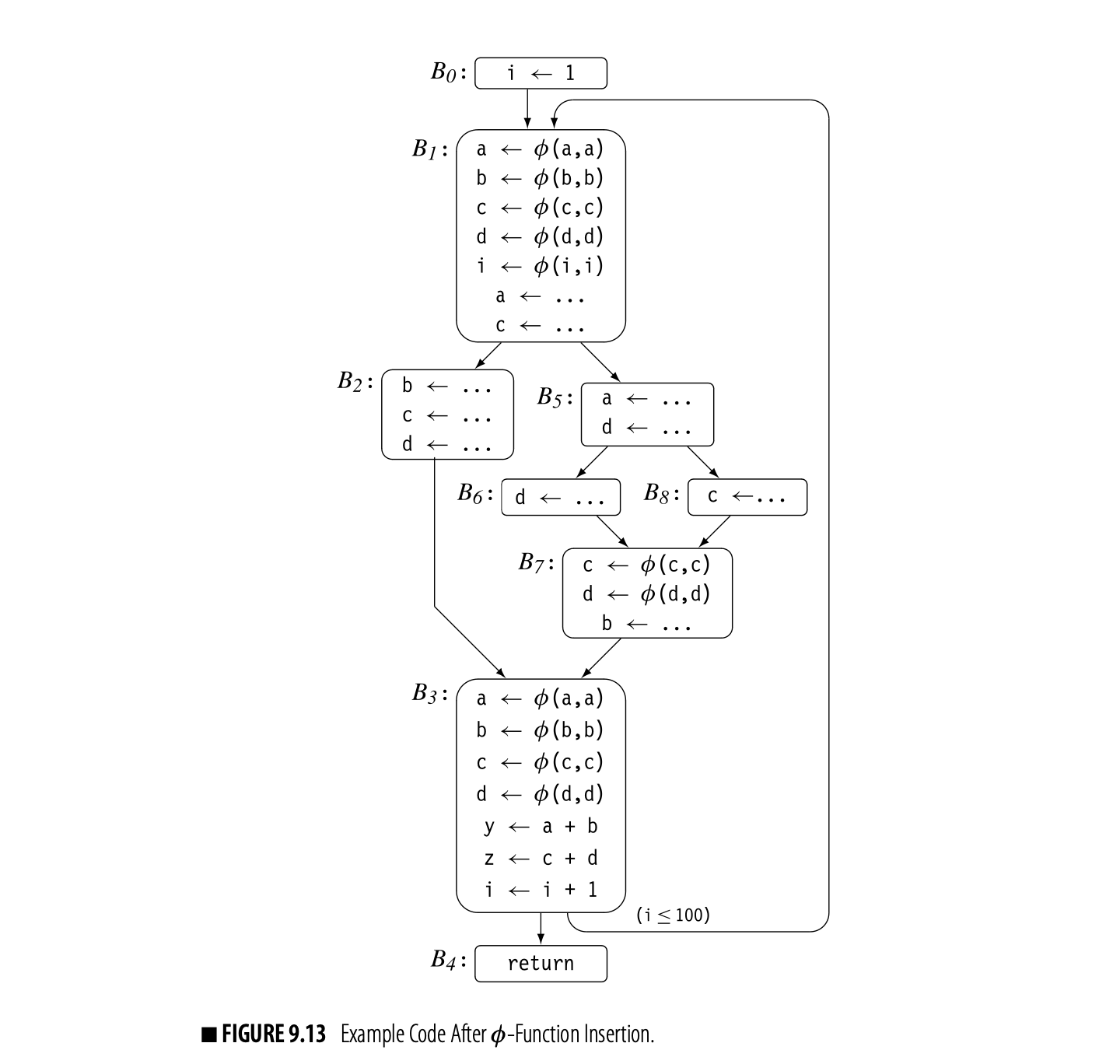
The algorithm follows the same logic for each name in Globols, to produce the following insertions:

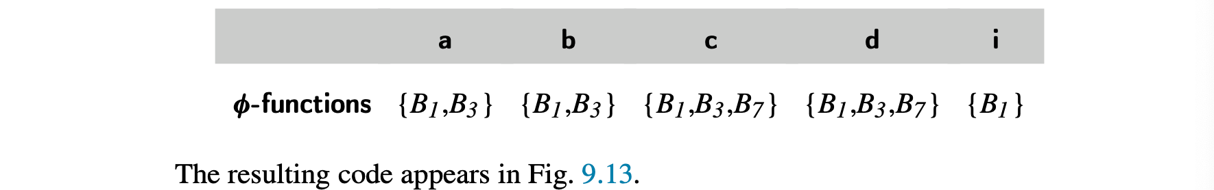
Limiting the algorithm to global names keeps it from inserting dead $ϕ$ -functions for $y$ and $z$ in block $B_{I}$ . ( $B_{I} \in DF (B_{3})$ and $B_{3}$ defines both $y$ and $z$ .) However, the distinction between local names and global names is not sufficient to avoid all dead $ϕ$ -functions. For example, the $ϕ$ -function for b in $B_{I}$ is not live because b is redefined before its value is used. To avoid inserting these $ϕ$ -functions, the compiler can construct LiveOut sets and add a test based on liveness to the inner loop of the $ϕ$ -function insertion algorithm. That modification causes the algorithm to produce $pruned SSA form$ .

Efficiency Improvements

To improve efficiency, the compiler should avoid two kinds of duplication. First, the algorithm should avoid placing any block on the worklist more than once per global name. It can keep a checklist of blocks that have already been processed for the current name and reset the checklist when it starts to process a new name.

Both of these checklists can be imple- mented as sparse sets (see Appendix B.2.3).

Second, a given block can be in the dominance frontier of multiple nodes that appear on the WorkList. The algorithm must check, at each insertion, for a preexisting $ϕ$ -function for the current name. Rather than searching through the $ϕ$ -functions in the block, the compiler should maintain a checklist of blocks that already contain $ϕ$ -functions for the current variable. Again, this checklist must be reset when the algorithm starts to process a new name.

9.3.4 Renaming

Earlier, we stated that the algorithm for renaming variables was conceptually straightforward. The details, however, require explanation.

In the final SSA form, each global name becomes a base name, and individual definitions of that base name are distinguished by the addition of a numerical subscript. For a name that corresponds to a source-language variable, say a, the algorithm uses a as the base name. Thus, the first definition of a that the renaming algorithm encounters will be named a0 and the second will be a1. For a compiler-generated temporary, the algorithm can use its pre-SSA name as its base name.

The algorithm, shown in Fig. 14, renames both definitions and uses in a preorder walk over the procedure's dominator tree. In each block, it first renames the values defined by $ϕ$ -functions at the head of the block. Next, it visits each operation in the block, in order. It rewrites the operands with current SSA names and then creates a new SSA name for the result of the operation. This latter act makes the new name current. After all the operations in the block have been rewritten, the algorithm rewrites the appropriate $ϕ$ -function parameters in each CFG successor of the block, using the current SSA names. Finally, it recurs on any children of the block in the dominator tree. When it returns from those recursive calls, it restores the set of current SSA names to the state that existed before the current block was visited.

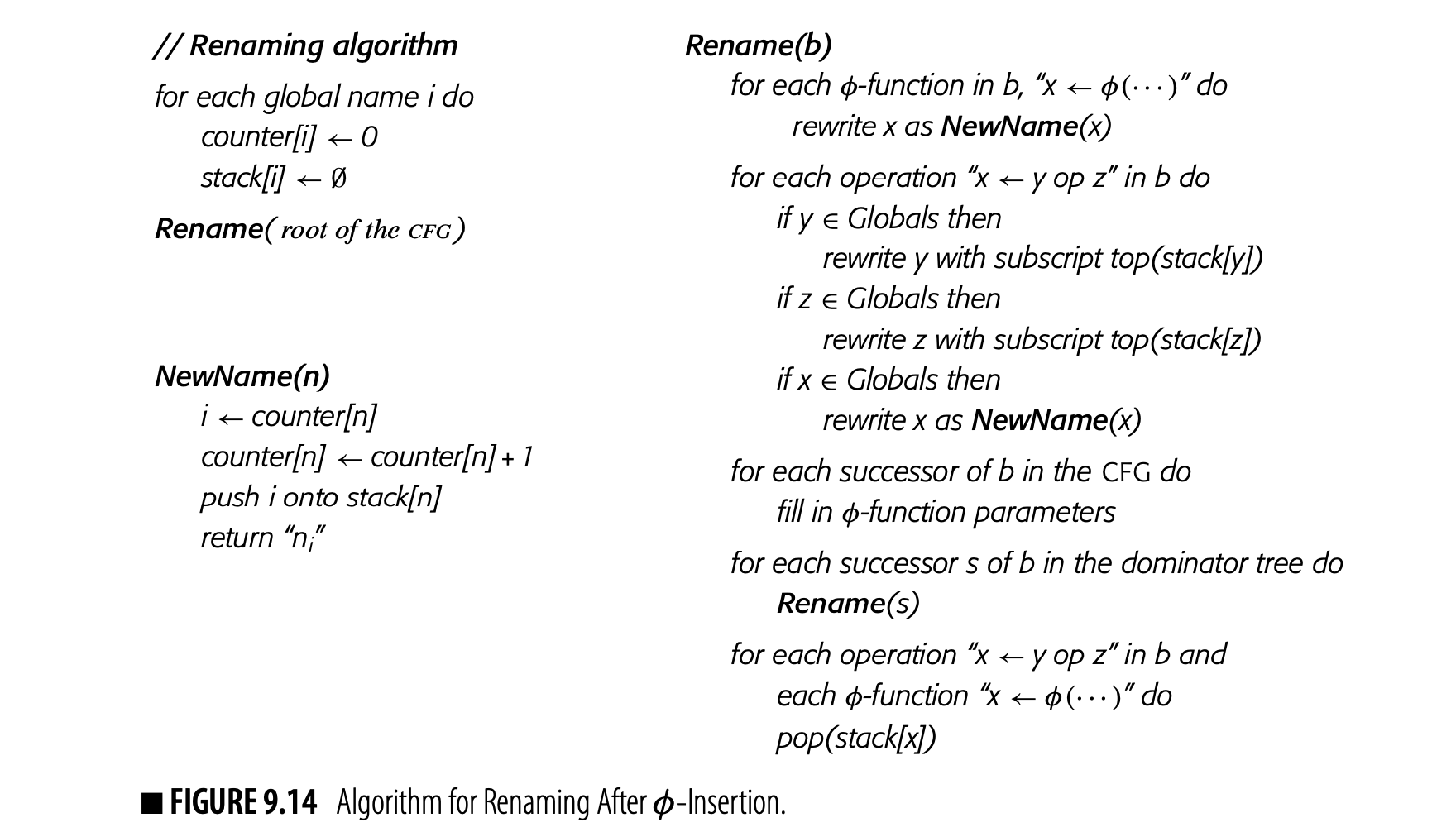
To manage the names, the algorithm uses a counter and a stack for each global name. A name's stack holds the subscript from its current SSA name. At each definition, the algorithm generates a new subscript for the defined base name by pushing the value of its current counter onto the stack and incrementing the counter. Thus, the value on top of the stack for $n$ is always the subscript of $n$ 's current SSA name.

As the final step, after recurring on the block's children in the dominator tree, the algorithm pops all the names generated in that block off their respective stacks. This action reveals the names that held at the end of that block's immediate dominator. Those names may be needed to process the block's remaining dominator-tree siblings.

The stack and the counter serve distinct and separate purposes. As the algorithm moves up and down the dominator tree, the stack is managed to simulate the lifetime of the most recent definition in the current block. The counter, on the other hand, grows monotonically to ensure that each successive definition receives a unique SSA name.

Fig. 9.14 summarizes the algorithm. It initializes the stacks and counters, then calls Rename on the dominator tree's root--the CFG's entry node. Rename processes the block, updates $ϕ$ -function arguments in its CFG successor blocks, and recurs on its dominator-tree successors. To finish the block, Rename pops off the stacks any names that it added as it processed the block. The function NewName manipulates the counters and stacks to create new SSA names as needed.

One final detail remains. When Rename rewrites the $ϕ$ -function parameters in each of $b$ 's CFG successors, it needs a mapping from $b$ to an ordinal parameter slot in those $ϕ$ -functions for $b$ . That is, it must know which parameter slot in the $ϕ$ -functions corresponds to $b$ .

When we draw SSA form, we assume a left-to-right order that matches the left-to-right order in which the edges are drawn. Internally, the compiler can number the edges and parameter slots in any consistent fashion that produces the desired result. This requires cooperation between the code that builds SSA and the code that builds the CFG. (For example, if the CFG implementation uses a list of edges leaving each block, the order of that list can determine the mapping.)

Example

To finish the continuing example, let's apply the renaming algorithm to the code in Fig. 9.13. Assume that $a_{0}$ , $b_{0}$ , $c_{0}$ , and $d_{0}$ are defined on entry to $B_{0}$ . Fig. 9.15 shows the states of the counters and stacks for global names at various points during the process.

The algorithm makes a preorder walk over the dominator tree, which, in this example, corresponds to visiting the nodes in ascending order by name. Fig. 9.15(a) shows the initial state of the stacks and counters. As the algorithm proceeds, it takes the following actions:

Block $B_{0}$ This block contains only one operation. Rename rewrites $i$ with $i_{0}$ , increments $i$ 's counter, and pushes $i_{0}$ onto the stack for $i$ . Next, it visits $B_{0}$ 's CFG-successor, $B_{I}$ , and rewrites the $ϕ$ -function parameters that correspond to $B_{0}$ with their current names: $a_{0}$ , $b_{0}$ , $c_{0}$ , $d_{0}$ , and $i_{0}$ . It then recurs on $B_{0}$ 's child in the dominator tree, $B_{I}$ . After that, it pops the stack for $1$ and returns.

Block $B_{1}$ Rename enters $B_{I}$ with the state shown in panel (b). It rewrites the $ϕ$ -function targets with new names, $a_{1}$ , $b_{1}$ , $c_{1}$ , $d_{1}$ , and $i_{1}$ . Next, it creates new names for the definitions of $a$ and $c$ and rewrites them. Neither of $B_{I}$ 's CFG successors have $ϕ$ -functions, so it recurs on $B_{I}$ 's dominator-tree children, $B_{2}$ , $B_{3}$ , and $B_{5}$ . Finally, it pops the stacks and returns.

Block $B_{2}$ Rename enters $B_{2}$ with the state shown in panel (c). This block has no $ϕ$ -functions to rewrite. Rename rewrites the definitions of $b$ , $c$ , and $d$ , creating a new SSA name for each. It then rewrites $ϕ$ -function parameters in $B_{2}$ 's CFG successor, $B_{3}$ . Panel (d) shows the stacks and counters just before they are popped. Finally, it pops the stacks and returns.

9.15.png

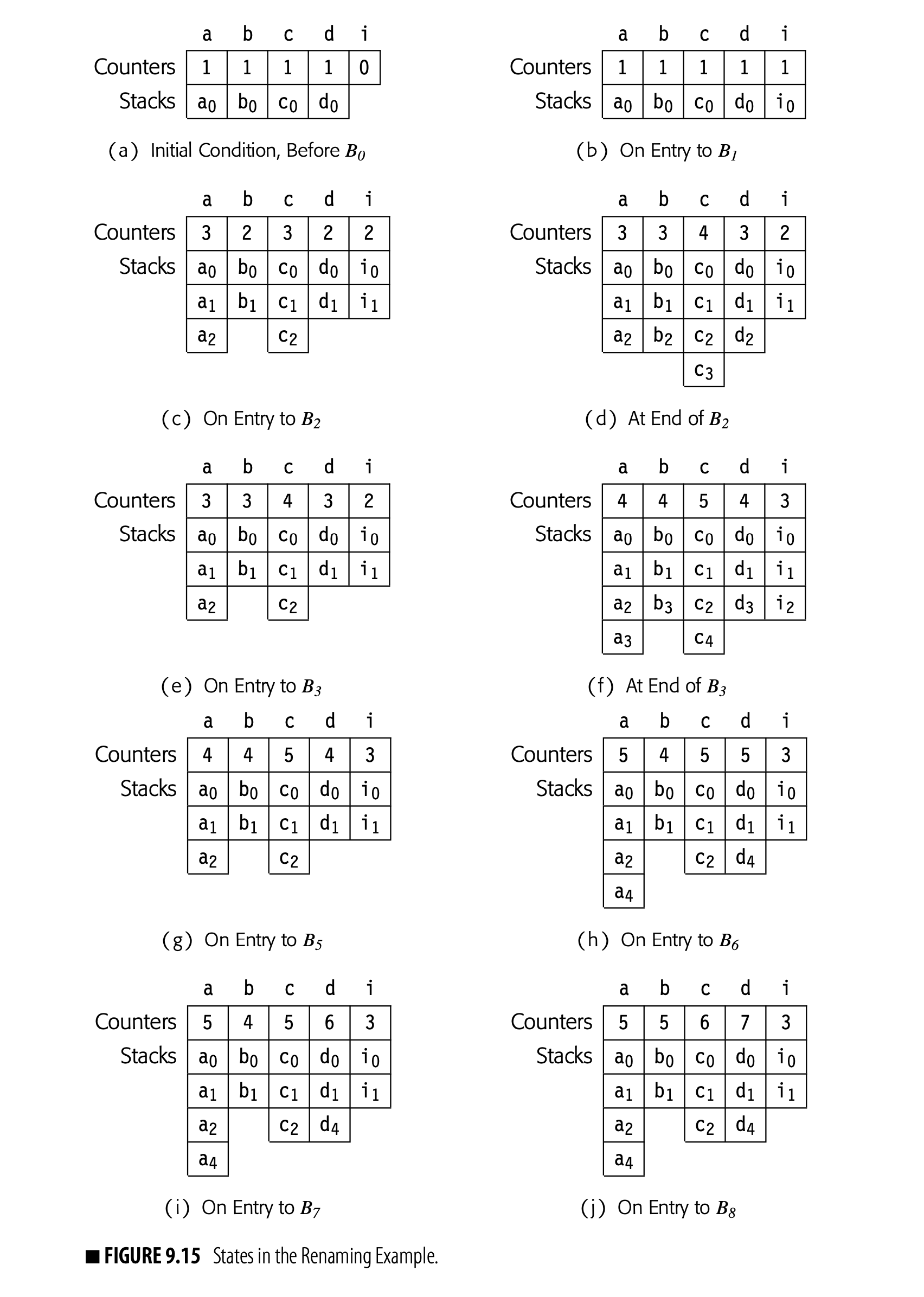
Block B3 Rename enters $B_{3}$ with the state shown in panel (e). Notice that the stacks have been popped to their state when Rename entered $B_{2}$ , but the counters reflect the names created inside $B_{2}$ . In $B_{3}$ , Rename rewrites the $ϕ$ -function targets, creating new SSA names for each. Next, it rewrites each assignment in the block, using current SSA names for the uses of global names and then creating new SSA names for definitions of global names. $B_{3}$ has two CFG successors, $B_{1}$ and $B_{4}$ . In $B_{1}$ , it rewrites the $ϕ$ -function parameters that correspond to the edge from $B_{3}$ , using the stacks and counters shown in panel (f). $B_{4}$ has no $ϕ$ -functions. Next, Rename recurs on $B_{3}$ 's dominator-tree child, $B_{4}$ . When that call returns, Rename pops the stacks and returns.

Block B4 This block just contains a return statement. It has no $ϕ$ -functions, definitions, uses, or successors in either the CFG or the dominator tree. Thus, Rename performs no actions and leaves the stacks and counters unchanged.

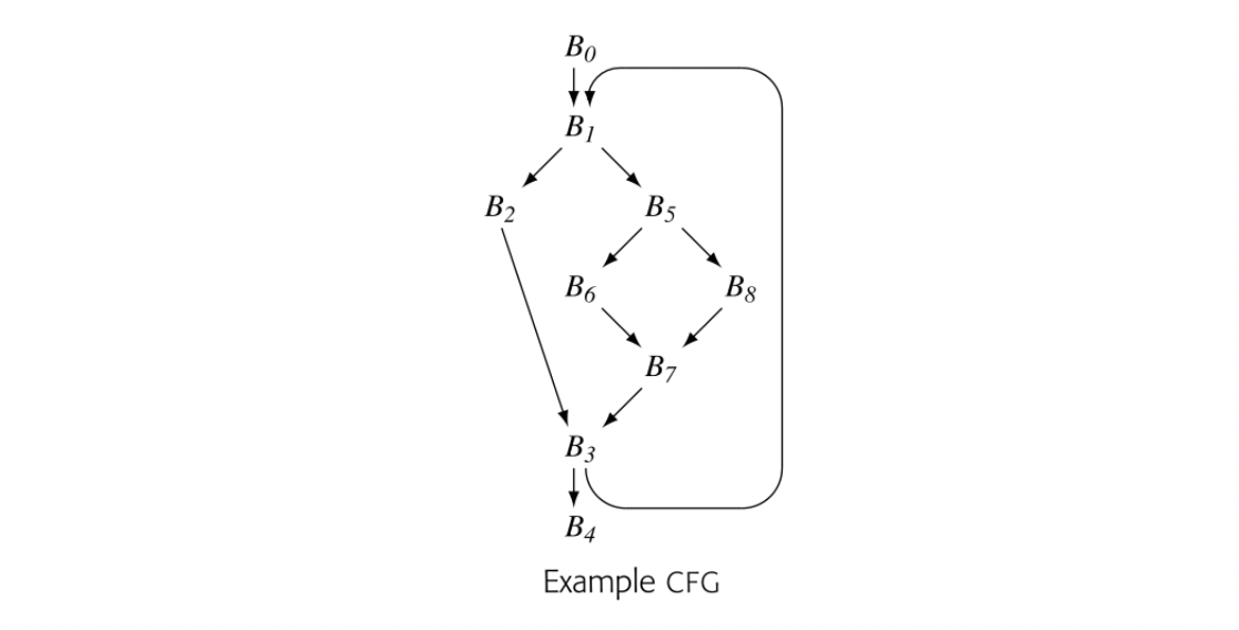
Block B5 After $B_{4}$ , Rename pops through $B_{3}$ back to $B_{1}$ . With the stacks as shown in panel (g), it recurs down into $B_{1}$ 's final dominator-tree child, $B_{5}$ . $B_{5}$ has no $ϕ$ -functions. Rename rewrites the two assignment statements, creating new SSA names as needed. Neither of $B_{5}$ 's CFG successors has $ϕ$ -functions. Rename next recurs on $B_{5}$ 's dominator-tree children, $B_{6}$ , $B_{7}$ , and $B_{8}$ . Finally, it pops the stacks and returns.

Block B6 Rename enters $B_{6}$ with the state in panel (h). $B_{6}$ has no $ϕ$ -functions. Rename rewrites the assignment to d, generating the new SSA name d5. Next, it visits the $ϕ$ -functions in $B_{6}$ 's CFG successor $B_{7}$ . It rewrites the $ϕ$ -function arguments along the edge from $B_{6}$ with their current names, $c_{2}$ and d5. Since $B_{6}$ has no dominator-tree children, it pops the stack for d and returns.

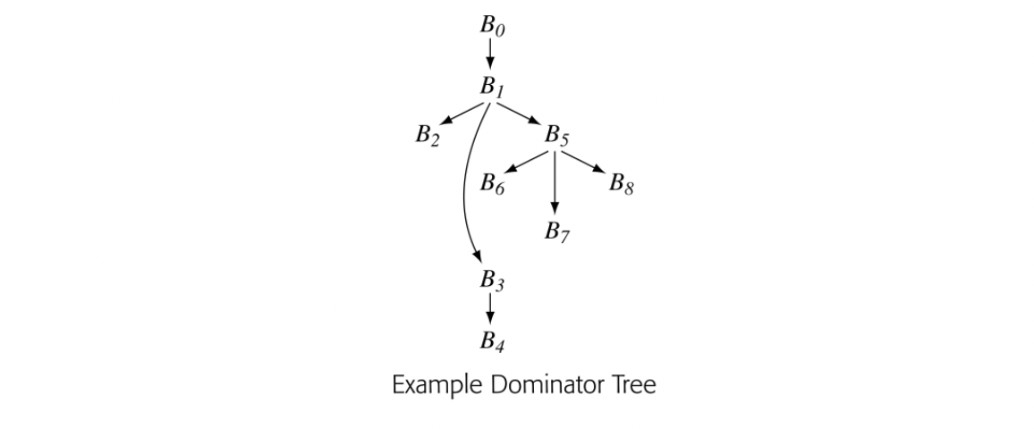Block B7 Rename enters $B_{7}$ with the state shown in panel (i). It first renames the $ϕ$ -function targets with new SSA names, $c_{5}$ and d6. Next, it rewrites the assignment to b with new SSA name b4. It then rewrites the $ϕ$ -function arguments in $B_{7}$ 's CFG successor, $B_{3}$ , with their current names. Since $B_{7}$ has no dominator-tree children, it pops the stacks and returns.

Block B8: Rename enters $B_{8}$ with the state shown in panel (j). $B_{8}$ has no $ϕ$ -functions. Rename rewrites the assignment to c with new SSA name c6. It rewrites the appropriate $ϕ$ -function arguments in $B_{7}$ with their current names, $c_{6}$ and d4. Since $B_{8}$ has no dominator-tree children, it pops the stacks and returns.

Fig 9.16 shows the code after Rename halts.

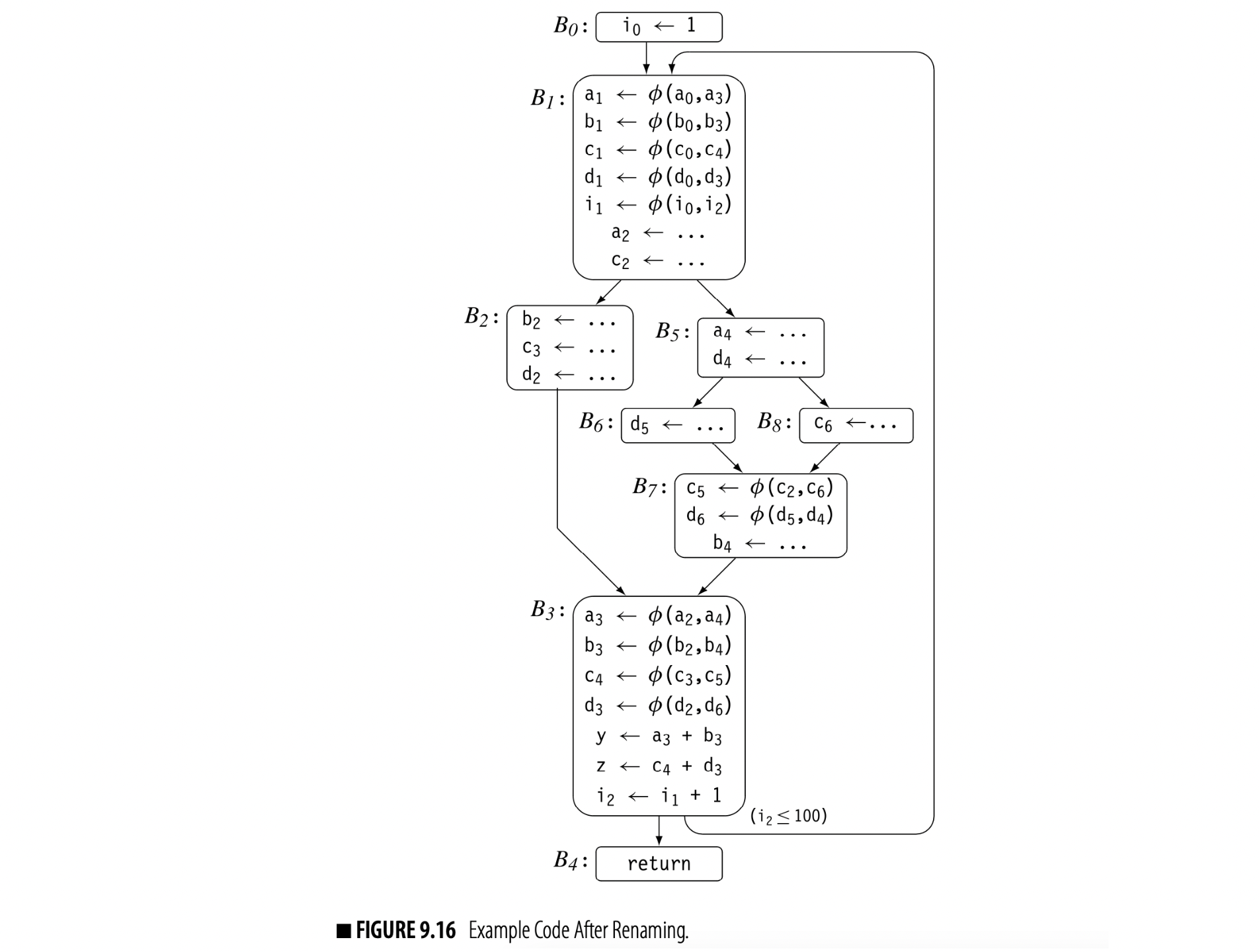
A Final Improvement

We can reduce the time and space spent in stack manipulation with a clever implementation of NewName. The primary use of the stacks is to reset the name space on exit from a block. If a block redefines the same base name multiple times, the stack only needs to keep the most recent name. For example, in block $B_{I}$ , both a and c are defined twice. NewName could reuse the slots for a $_{1}$ and c $_{1}$ when it creates a $_{2}$ and c $_{2}$ .

With this change, Rename performs one push and one pop per base name defined in the block. NewName can keep a list of the stack entries that it creates; on exit from the block, Rename can then walk the list to pop theappropriate stacks. The stacks require less space; their size is bounded by the depth of the dominator tree. Stack manipulation is simplified; the algorithm performs fewer push and pop operations and the push operation need not test for a stack overflow.

9.3.5 Translation out of SSA Form

Actual processors do not implement φ- functions, so the compiler must rewrite the code without the φ-functions.

A compiler that uses SSA form must translate that form of the code back into a more conventional model--one without $ϕ$ -functions--before the code can execute on conventional computer hardware. The compiler must replace the $ϕ$ -functions with copy operations and place them in the code so that they reproduce the semantics of those $ϕ$ -functions: both the control-based selection of values and the parallel execution at the start of the block.

This section addresses out-of-SA translation. It begins with an overly simple, or naive, translation, which informs and motivates the actual translation schemes. Next, it presents two example problems that demonstrate the problems that can arise in translating from SSA form back to conventional code. Finally, it presents a unified framework that addresses the known complexities of the translation.

The Naive Translation

A $ϕ$ -function is just a copy operation that selects its input based on prior control-flow. To replicate the effect of a $ϕ$ -function at the top of block $b$ , the compiler can insert, at the end of each CFG-predecessor of $b$ , a copy operation that moves the appropriate $ϕ$ -function argument into the name defined by the $ϕ$ -function (shown in the margin). Once the compiler has inserted the copies, it can delete the $ϕ$ -function.

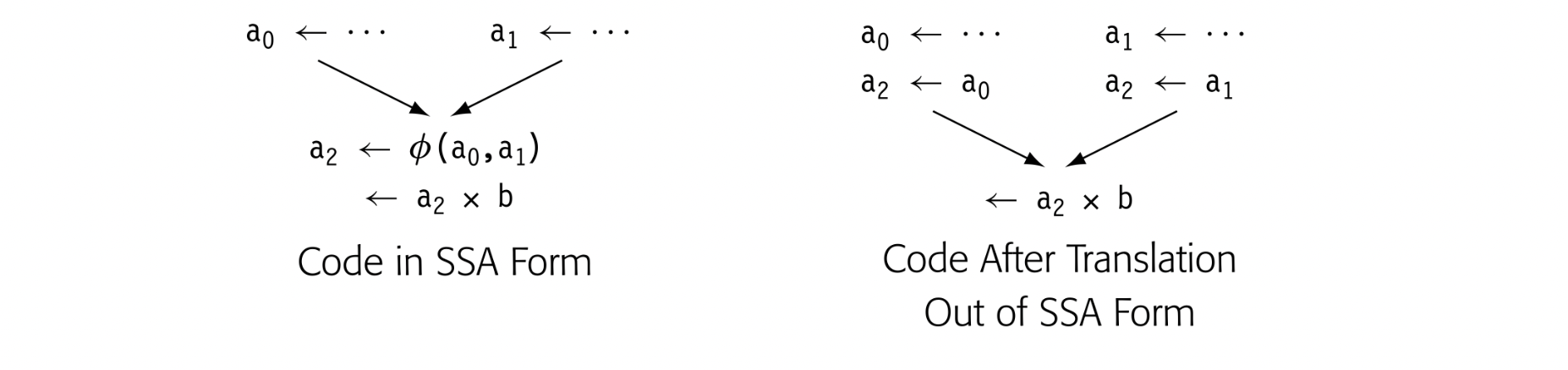
This process, while conceptually simple, has some complications. Consider, for example, the continuing example from Fig. 16. Three blocks in the CFG contain $ϕ$ -functions: $B_{1}$ , $B_{3}$ , and $B_{7}$ . Fig. 17 shows the code after copies have been inserted.

For $B_{3}$ and $B_{7}$ , insertion into the predecessor blocks works. The predecessors of both $B_{3}$ and $B_{7}$ have one successor each, so the copy operations inserted at the end of those predecessor blocks have no effect on any path other than the one to the $ϕ$ -function.

The situation is more complex for $B_{1}$ . Copy insertion at the end of $B_{1}$ 's predecessor, $B_{0}$ , produces the desired result; the copies only occur on the path $(B_{0}, B_{1})$ . With $B_{1}$ 's other predecessor, $B_{3}$ , simple insertion will not work. A copy inserted at the end of $B_{3}$ will execute on both $(B_{3}, B_{1})$ and $(B_{3}, B_{4})$ . Along $(B_{3}, B_{4})$ , the copy operation may change a value that is live in $B_{4}$ .

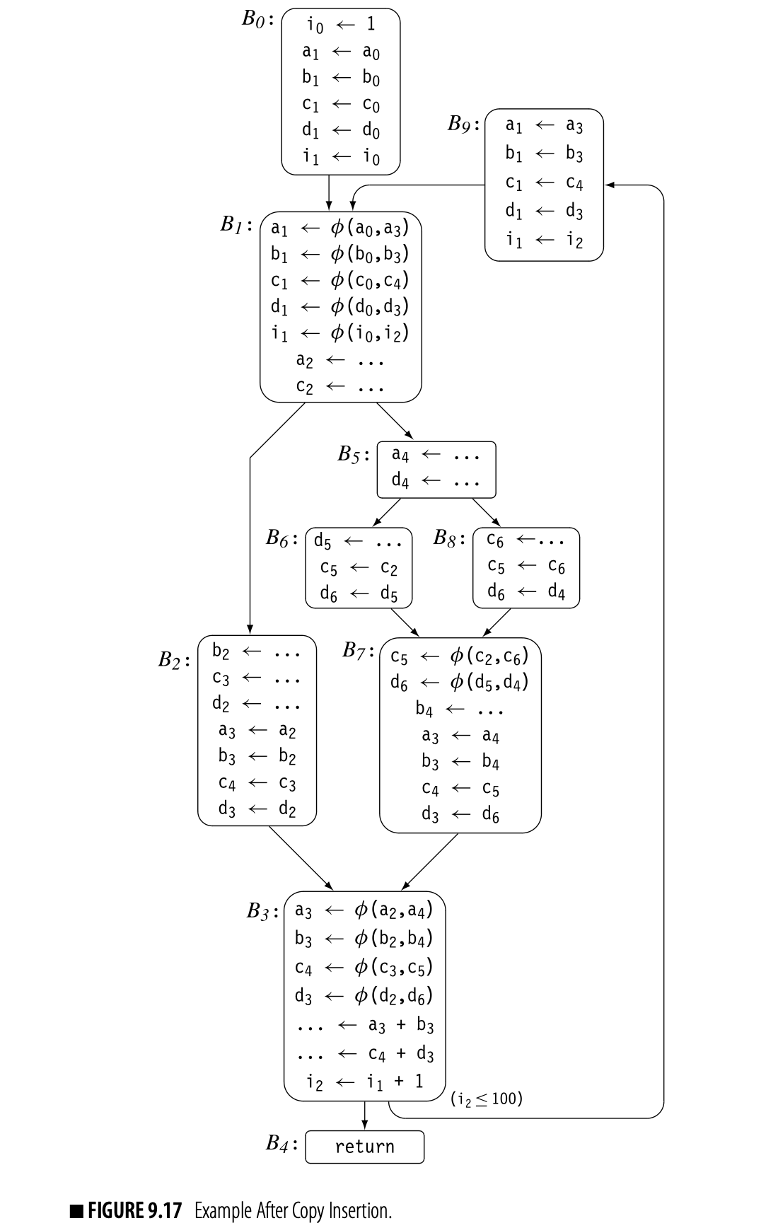
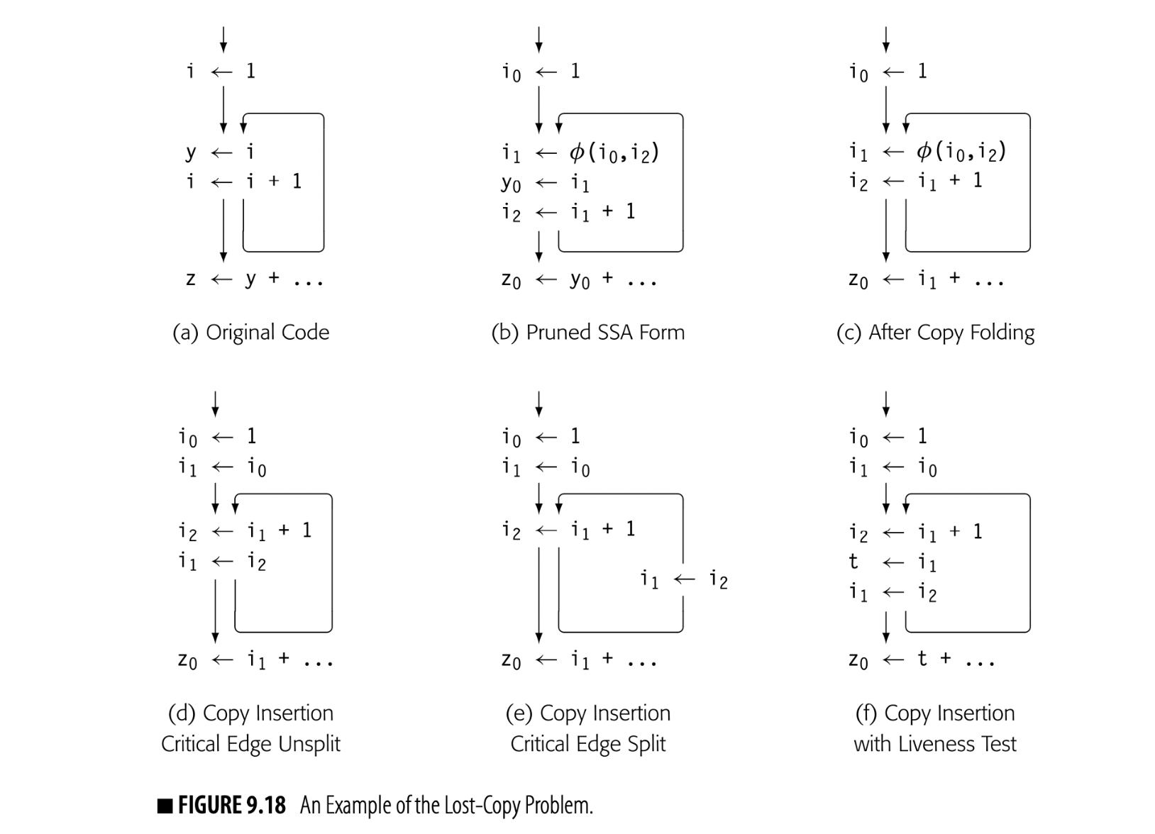
Critical edge A flow graph $e d g e (i, j)$ is a critical edge if $i$ has multiple successors and $j$ has multiple predecessors. Optimizations that move or insert code often need to split critical edges.

The edge $(B_{3}, B_{1})$ highlights a more general problem with code placement on a critical edge. $B_{3}$ has multiple successors, so the compiler cannot insert the copy at the end of $B_{3}$ . $B_{1}$ has multiple predecessors, so the compiler cannot insert the copy at the start of $B_{I}$ . Since neither solution works, the compiler must split the edge and create a new block to hold the inserted copy operations. With the split edge and the creation of $B_{9}$ , the translated code faithfully reproduces the effects of the SSA form of the code.

Problems with the Naive Translation

If the compiler applies the naive translation to code that was produced directly by the translation into SSA form, the results will be correct, as long as critical edges can be split. If, however, the compiler transforms the code while it is in SSA form--particularly, transformations that move definitions or uses of SSA names--or if the compiler cannot split critical edges, then the naive translation can produce incorrect code. Two examples demonstrate how the naive translation can fail.

The Lost-Copy Problem

In Fig. 9.17, the compiler had to split the edge $(B_{3}, B_{1})$ to create a location for the copy operations associated with that edge. In some situations, the compiler cannot or should not split a critical edge. For example, an SSA-based register allocator should not add any blocks or edges during copy insertion (see Section 13.5.3). The combination of an unsplit critical edge and an optimization that extends some SSA-name's live range can create a situation where naive copy insertion fails.

Fig. 9.18(a) shows an example to demonstrate the problem. The loop increments $i$ . The computation of $z$ after the loop uses the second-to-last value of $i$ . Panel (b) shows the pruned SSA for the code.

Panel (c) shows the code after copy folding. The use of $y_{0}$ in the computation of $z_{0}$ has been replaced with a use of $i_{1}$ . The last use of $i_{1}$ in panel (b) was in the assignment to $y_{0}$ ; folding the copy extends the live range of $i_{1}$ beyond the end of the loop in panel (c).

Copy folding an optimization that removes unneeded copy operations by renaming the source and destination to the same name, when such renaming does not change the flow of values $Copy folding$ is also called $copy coalescing$ (see Section 13.4.3).

Copy insertion on the code in panel (c) adds $i_{1} \leftarrow i_{0}$ to the end of the preloop block, and $i_{1} \leftarrow i_{2}$ at the end of the loop. Unfortunately, that latter assignment kills the value in $i_{1}$ ; the computation of $z_{0}$ now receives the final value of $i$ rather than its penultimate value. Copy insertion produces incorrect code because it extends $i_{1}$ 's live range.

Splitting the critical edge cures the problem, as shown in panel (e); the copy does not execute on the loop's final iteration. When the compiler cannot split that edge, it must add a new name to preserve the value of $i_{1}$ , as shown in panel (f). A simple, ad-hoc addition to the copy insertion process can avoid the lost-copy problem. As the compiler inserts copies, it should check whether or not the target of the new copy is live at the insertion point. If the target is live, the compiler must introduce a new name, copy the live value into it, and propagate that name to the uses after the insertion point.

The Swap Problem

The concurrent semantics of $ϕ$ -functions create another problem for out-of-SSA translation, which we call the swap problem. The motivating example appears in Fig. 9.19(a): a simple loop that repeatedly swaps the values of $x$ and $y$ . If the compiler builds pruned SSA-form, as in panel (b), and performs copy folding, as in panel (c), it creates a valid program in SSA form that relies directly on the concurrent semantics of the $ϕ$ -functions in a single block.

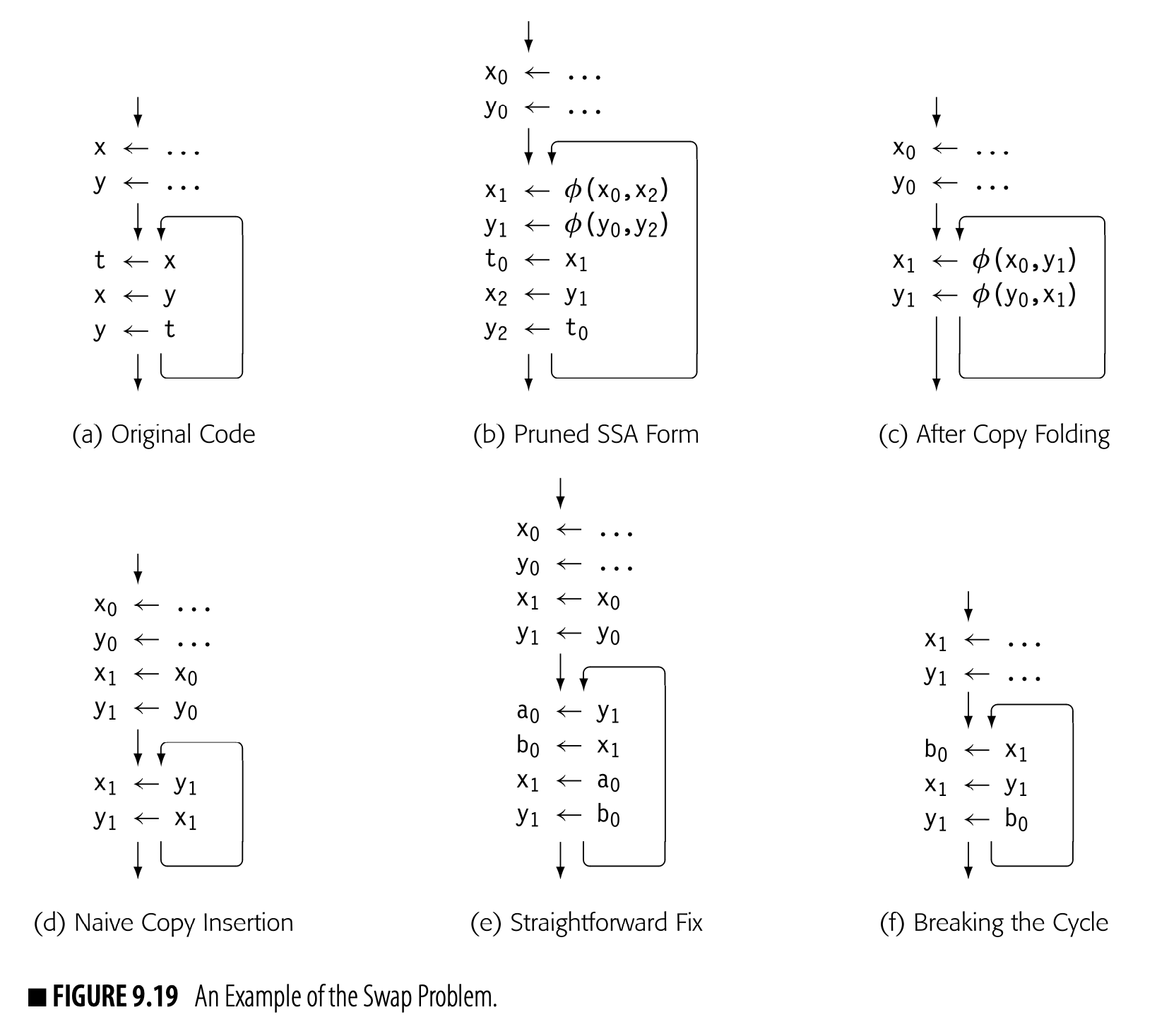
Because the two $ϕ$ -functions read their values concurrently and then write their results concurrently, the code in panel (c) has the same meaning as theoriginal code from panel (a). Naive copy-insertion, however, replaces each $ϕ$ -function with a sequential copy operation, as shown in panel (d). The two sequential copies have a different result than did the two $ϕ$ -functions; the substitution fundamentally changes the meaning of the code.

To maintain the original code's meaning, the compiler must ensure that the inserted copies faithfully reproduce the flow of values specified by the $ϕ$ -functions. Thus, it must pay attention to any values that are defined by one $ϕ$ -function and used by another $ϕ$ -function in the same block.

In some cases, the compiler must introduce one or more new names. The straightforward solution to this problem is to adopt a two-stage copy protocol, as shown in panel (e). The first stage copies each of the $ϕ$ -function arguments into its own temporary name, simulating the control-based selection and the parallel read of the $ϕ$ -function. The second stage then copies those values to the $ϕ$ -function targets.

Unfortunately, this solution doubles the number of copy operations required to translate out of SSA form. The compiler can reduce the number of temporary names and extra copy operations by building a small dependence graph for the set of parallel copies implied by the $ϕ$ -functions and using the graph to guide insertion of the sequential copies. If the dependence graph is acyclic, then the compiler can use it to schedule the copy operations in a way that requires no additional names or operations (see Chapter 12).

If the dependence graph contains cycles, then the compiler must break each cycle with a copy into a name not involved in the cycle. This may require a new name. The dependence graph for the example, shown in the margin, consists of a two node cycle. It requires one new name to break the cycle, which produces the code shown in panel (f).

A Unified Approach to Out-of-SSA Translation

The swap problem and the copy problem arise from two distinct phenomena: transformations that change the range over which an SSA-name is live, and failure to preserve the parallel semantics of $ϕ$ -function execution during translation out of SSA-form. Common code transformations, such as copy folding, code motion, and cross-block instruction scheduling, can create the circumstances that trigger these problems. While the solutions proposed in the previous section will generate correct code, neither solution provides a clean framework for understanding the underlying issues.

The unified approach uses a three-phase plan to address the two issues caused by code transformations on the SSA form: changes in the live ranges of SSA names and implicit use of the parallel semantics of $ϕ$ -function execution. Phase one introduces a new set of names to isolate $ϕ$ -functions from the rest of the code; it then inserts parallel copy operations to connect those names with the surrounding context. Phase two replaces $ϕ$ -functions with parallel copy operations in predecessor blocks. Phase three rewrites each block of parallel copies with an equivalent series of sequential copies. This process avoids both the swap problem and the lost copy problem. At the same time, it eliminates the need to split critical edges.

Phase One

We will denote a parallel copy group by adding a common subscript to the assignment operator, $\leftarrow_{i}$ .

To isolate the name space for a $ϕ$ -function, such as $a_{0} \leftarrow ϕ (a_{1}, a_{2}, \dots, a_{n})$ , phase one rewrites it as $a_{0}^{'} \leftarrow ϕ (a_{1}^{'}, a_{2}^{'}, \dots, a_{n}^{'})$ . To connect the new primed names with the surrounding code, the compiler adds a copy operation $a_{i}^{'} \leftarrow a_{i}$ to the end of the predecessor block associated with $a_{i}$ , for each parameter $a_{i}$ . To retain the parallel execution semantics of the $ϕ$ -functions, the compiler will use parallel copy groups for the copies that it inserts.

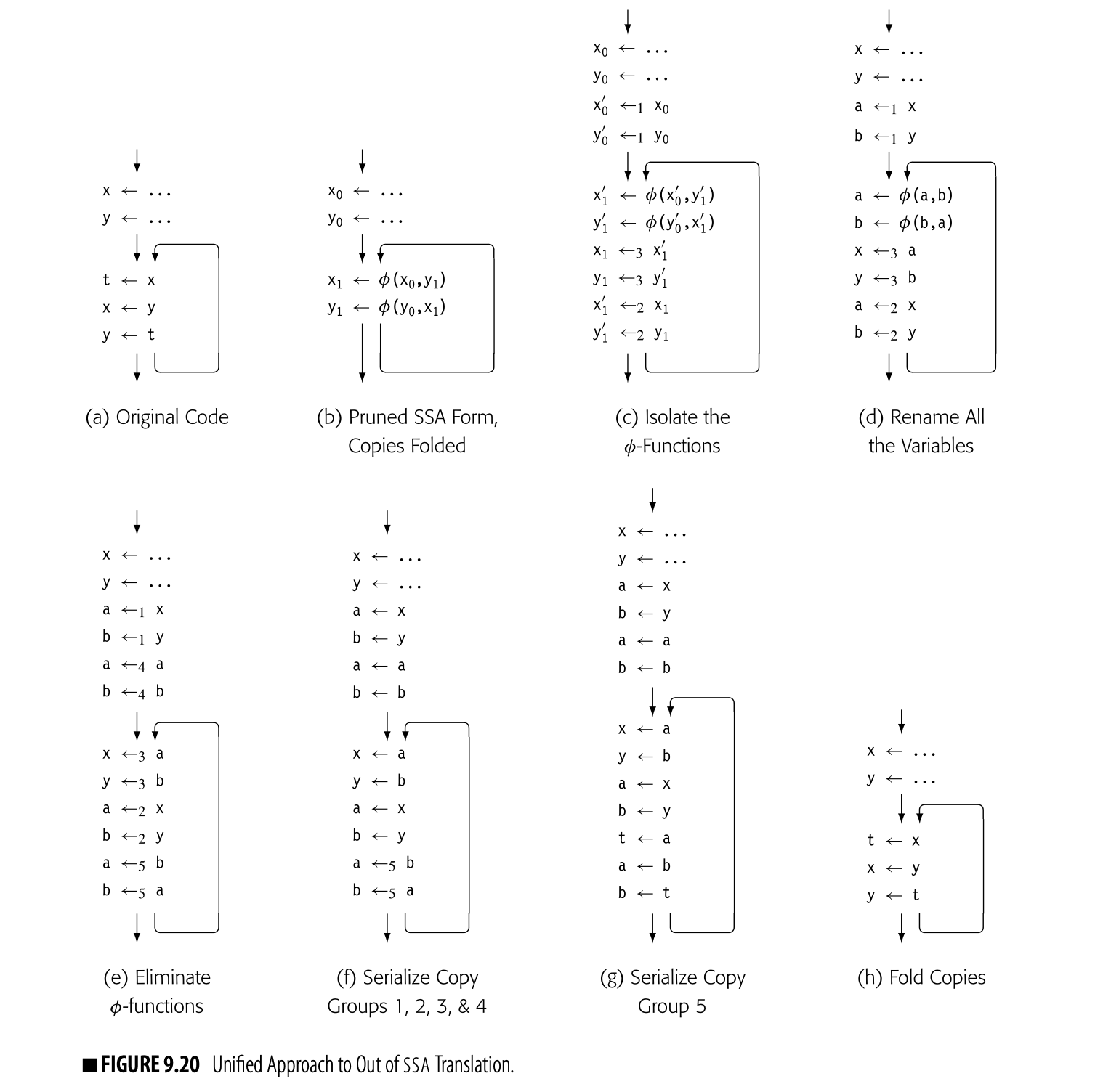
After the group of $ϕ$ -functions at the head of a block, the compiler should insert another parallel copy group. For each $ϕ$ -function in the block, $a_{i} \leftarrow ϕ (\dots)$ , the copy group should include a copy of the form $a_{i} \leftarrow a_{i}^{'}$ . The net effect of these three actions is to isolate the names used in the $ϕ$ -functions from the surrounding code and to make the impact of parallel execution explicit, outside of the $ϕ$ -functions. Fig. 9.20 shows the effects of this transformation on the example from the swap problem. Panel (a) shows the original code; panel (b) shows it in pruned ssa form, with copies folded. Panel (c) shows the code after the compiler has isolated the $ϕ$ -functions. The $ϕ$ -function parameters have been renamed and parallel copy groups inserted.

Parallel copy group 1, at the end of the first block, gives $x_{0}^{'}$ and $y_{0}^{'}$ their initial values.
Parallel copy group 2, at the end of the loop body, gives $x_{1}^{'}$ and $y_{1}^{'}$ their values from computation inside the loop. (The loop body is its own predecessor.)
Parallel copy group 3, after the $ϕ$ -functions, copies the values defined by the $ϕ$ -functions into the names that they had before the renaming transformation. At this point, the compiler can rename all of the primed variables and drop all of the subscripts from SSA names, as shown in panel (d). The renamed code retains the meaning of the original code.

Phase Two

This phase replaces $ϕ$ -functions by inserting copies into predecessor blocks and deleting the $ϕ$ -functions. To retain the $ϕ$ -function semantics, the compiler uses parallel copies in each block.

At the end of phase one as shown in panel (d), the actual value swap occurs during evaluation of the $ϕ$ -function arguments. After $ϕ$ -function replacement, shown in panel (e), that value swap occurs in parallel copy group 5, at the end of the loop body.

At the end of phase two, the compiler has eliminated all of the $ϕ$ -functions. The code still contains groups of parallel copy operations that implement the semantics of the $ϕ$ -functions. To complete the process, the compiler must rewrite each parallel copy group into a set of serial copies. The code will likely contain multiple (perhaps many) unneeded copy operations. Coalescing can eliminate some or all of them (see Section 13.4.3).

Phase Three

The final phase examines each parallel copy group and rewrites it with an equivalent group of sequential copy operations. It builds a data-dependence graph for the copy group (see Section 4.3.2). If the graph is acyclic, as in the acyclic graph shown in the margin, the compiler can simply insert copies in the order implied by the graph--leaves to roots. For the first example, the graph requires that $a \leftarrow b$ and $d \leftarrow b$ precede $b \leftarrow c$ . If the dependence graph contains a cycle, as shown in the example in the margin, the compiler must insert copies in a way that breaks the cycle. In the example, it must copy one of the values, say a, into a new temporary name, say t. Then, it can perform a $\leftarrow$ b and b $\leftarrow$ c. It can finish the copy group with c $\leftarrow$ t. This breaks the cycle and correctly implements the semantics of teh parallel copy group. In some cases, the compiler can avoid the new name by careful ordering. For example, if the second example also included a copy d $\leftarrow_{2}$ a, the compiler could schedule d $\leftarrow$ a first and break the cycle by rewriting c $\leftarrow$ a as c $\leftarrow$ d.

In the example, groups 1, 2, 3, and 4 can be serialized without additional names, as shown in panel (f). Copy group 5 contains a cycle, so it requires one new name, t. Panel (g) shows the rewrite of copy group 5. Panel (h) shows the final code after copy folding.

9.3.6 Using SSA Form

A compiler writer uses SSA form because it improves the quality of analysis, the quality of optimization, or both. To see how analysis on SSA differs from the classical data-flow analysis techniques presented in Section 9.2, consider the problem of global constant propagation on SSA, using an algorithm called sparse simple constant propagation (SSCP).

Semilattice a set $L$ and a $m ee t$ operator $\land$ such that, $\forall$ a, b, and $c \in L$ ,

$a \land a = a$ ,
$a \land b = b \land a$ , and
$a \land (b \land c) = (a \land b) \land c$ Compilers use semilattices to model the data domains of analysis problems.

In SSCP, the compiler annotates each SSA name with a value. The set of possible values forms a semilattice. A semilattice consists of a set $L$ of values and a meet operator, $\land$ . The meet operator must be idempotent, commutative, and associative; it imposes an order on the elements of $L$ :

Every semilattice has a bottom element, $⊥$ , with the properties that Some semilattices also have a top element, $⊤$ , with the properties that In constant propagation, the structure of the semilattice used to model program values plays a critical role in the algorithm's runtime complexity. The semilattice for a single SSA name appears in the margin. It consists of $⊤$ , $⊥$ , and an infinite set of distinct constant values. For any value $x$ : $x \land ⊤ = x$ , and $x \land ⊥ = ⊥$ . For two constants, $c_{i}$ and $c_{j}$ : $c_{i} \land c_{j} = ⊥$ if $c_{i} \neq = c_{j}$ . If $c_{i} = c_{j}$ , then $c_{i} \land c_{j} = c_{i}$ .

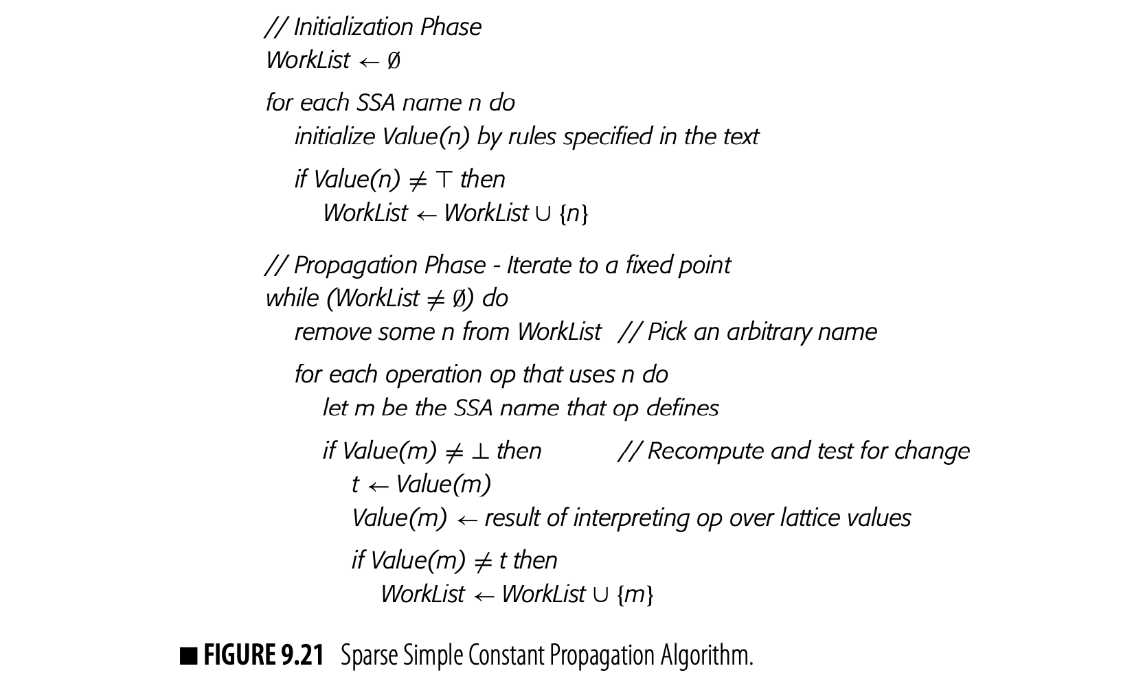The algorithm for SSCP, shown in Fig. 9.21, consists of an initialization phase and a propagation phase. The initialization phase iterates over the SSA names. For each SSA name $n$ , it examines the operation that defines $n$ and sets $Value(n)$ according to a simple set of rules.

If n is defined by a \phi-function, \operatorname{SSCP} sets \operatorname{Value}(n) to T.
if n 's value is not known, \operatorname{SSCP} sets \operatorname{Value}(n) to T.
If n 's value is a known constant c_{i}, \operatorname{SSCP} sets Value (n) to c_{i}.
If n 's value cannot be known-for example, it is defined by reading a value from external media—SSCP sets \operatorname{Value}(n) to \perp.

If Value (n) is not T, the algorithm adds n to the worklist.

These initializations highlight the use of T and $⊥$ in the constant propagation semilattice. T indicates that the compiler does not yet know anything about the value, but that it might discover information about its value in the future. By contrast, $⊥$ indicates that the compiler has proven that the value is not a constant. For any SSA name m, $Value(m)$ can change at most twicethe height of the semilattice. If $Value(m)$ starts as $T$ , it can progress to some constant $c_{i}$ or to $⊥$ . If $Value (m)$ is some constant $c_{i}$ , it can progress to $⊥$ . Once $Value(m)$ is $⊥$ , it cannot change.

The propagation phase is straightforward. It removes an SSA name n from the worklist. The algorithm examines each operation op that uses n, where op defines some SSA name m. If $Value(m)$ has already reached $⊥$ , then no further evaluation is needed. Otherwise, it models the evaluation of op by interpreting the operation over the lattice values of its operands. If the result is lower in the lattice than $Value(m)$ , it lowers $Value(m)$ accordingly and adds m to the worklist. The algorithm halts when the worklist is empty.

Interpreting an operation over lattice values requires some care. For a $ϕ$ -function, the result is simply the meet of the lattice values of all the $ϕ$ -function's arguments; the rules for meet are shown in the margin, in order of precedence. For other kinds of operations, the compiler needs a set of rules. Consider, for example, $a \times b$ . If $a = 4$ and $b = 17$ , then $a \times b = 68$ . However, if $a = ⊥$ , then $a \times b = ⊥$ , unless $b = 0$ . ( $a \times 0 = 0$ , for any $a$ .)

In general, the evaluation rules for operators should preserve $⊤$ , unless the other operand forces a value, as with multiplication by zero. If $a = ⊤$ , then evaluating $a + b$ to $⊤$ will defer determination of the sum until $a$ 's value is resolved to either a constant or $⊥$ .

Complexity

The propagation phase of SSCP is a classic fixed-point scheme. The arguments for termination and complexity follow from the length of descending chains through the semilattice, shown again in the margin. The lattice value for an SSA name can change at most twice: from $⊤$ to $c_{1}$ and from $c_{1}$ to $⊥$ . SSCP only adds an SSA name to the worklist when its value changes, so each name appears on the worklist at most twice. SSCP evaluates an operation when one of its operands is removed from the worklist, which bounds the number of evaluations at twice the number of uses in the code.

Optimism: The Role of Top

As discussed earlier, SSCP uses the lattice value $⊤$ to represent a lack of knowledge. This practice differs from the data-flow problems in Section 9.2, which use the value $⊥$ but not the value $⊤$ . The use of $⊤$ as an initial value plays a critical role in constant propagation; it allows values to propagate into cycles in the graph.

Because it initializes unknown values to $⊤$ , rather than $⊥$ , it can propagate some values into cycles in the graph--loops in the CFG. Algorithms that begin with the value $⊤$ , rather than $⊥$ , are often called optimistic algorithms. The intuition behind "optimism" is that initialization to $⊤$ allows the algorithm to propagate information into a cyclic region, optimistically assuming that the value along the back edge will confirm this initial propagation. An initialization to $⊥$ , called pessimistic, disallows that possibility.

Consider the SSA fragment in Fig. 9.22. If the algorithm initializes $x_{1}$ and $x_{2}$ to $⊥$ (pessimism), it will not propagate the value $17$ into the loop. When it evaluates the $ϕ$ -function, it sets $x_{1}$ to $17 \land ⊥ = ⊥$ . Once $x_{1} = ⊥$ , propagation sets $x_{2} = ⊥$ , independent of $i_{12}$ 's value.

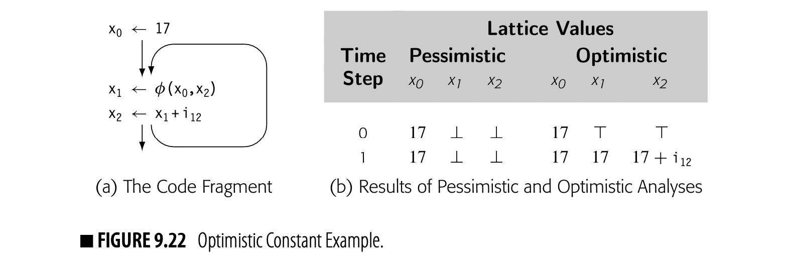
If, on the other hand, the algorithm initializes $x_{1} = ⊤$ and $x_{2} = ⊤$ (optimism), it can propagate $x_{0}$ 's value into the loop. It computes $x_{1}$ 's value as $17 \land ⊤ = 17$ . Since $x_{1}$ 's value has changed, the algorithm places $x_{1}$ on WorkList. The algorithm then reevaluates the definition of $x_{2}$ . If, for example, $i_{12} = 0$ , then $x_{2}$ gets the value $17$ and the algorithm adds $x_{2}$ to the worklist. When it reevaluates the $ϕ$ -function, it sets $x_{1} = 17 \land 17 = 17$ .

Consider what would happen if $i_{12} = 2$ , instead. Then, when SSCP evaluates $x_{1} + i_{12}$ it sets $x_{2} = 19$ . Next, it reevaluates $x_{1} = 17 \land 19 = ⊥$ . This $⊥$ , in turn, propagates to $x_{2}$ , proving $x$ nonconstant in the loop.

The Value of SSA Form

The use of SSA form in SSCP leads to a simple and efficient algorithm. To see this point, consider a classic data-flow approach to the problem. It would create a set ConstantsIN at the top of each block and a set ConstantsOut at the end of each block. ConstantsIN and ConstantsOut would hold $⟨ variable, value ⟩$ pairs.

This sketch oversimplifies the algorithm. This formulation lacks a unique fixed point, so the results depend on the order in which the blocks are processed. It also lacks the properties that let the iterative algorithm converge quickly. Solvers may run in $O (n 2$ ) time, or worse.

For a block $b$ , the compiler could compute $C o n s t an t s I N ($ b $)$ as a pairwise intersection of ConstantsOut( $p$ ), taken over every $p \in preds (b)$ . All the values for a single name would be intersected using the same meet function as in SSCP. To derive ConstantsOut( $b$ ) from ConstantsIN( $b$ ) the compiler could apply a version of LVN extended to handle $⊥$ and $⊤$ . An iterative fixed-point algorithm would halt when the sets stopped changing.

By contrast, SSCP is a simple iterative fixed-point algorithm operating on a sparse graph and particularly shallow lattice. It has the same complication with interpreting each operation over the known constant values, but it interprets single operations rather than whole blocks. It has an easily understood time bound. In this case, use of SSA form leads directly to a simple, efficient, sparse method for global constant propagation.

Section Review

SSA form encodes information about both data flow and control flow in a conceptually simple intermediate form. This section focused on the algorithms to translate code into and out of semipruned SSA form. The initial construction of SSA form is a two-step process. The first step inserts $ϕ$ -functions into the code at join points where distinct definitions can converge. That algorithm relies on dominance frontiers for efficiency. The second step creates the SSA name space by adding subscripts to the original base names during a systematic traversal of the entire procedure.

Because processors do not directly implement $ϕ$ -functions, the compiler must translate code out of SSA form before it can execute. Transformation of the code while in SSA form can complicate out-of-SSA translation. Section 9.3.5 examined both the "lost copy problem" and the "swap problem" and described approaches for handling them. Finally, Section 9.3.6 showed an algorithm for global constant propagation over the SSA-form.

Review Questions

Maximal SSA form includes useless $ϕ$ -functions that define nonlive values and redundant $ϕ$ -functions that merge identical values ( $e.g., x_{8} \leftarrow ϕ (x_{7}, x_{7}))$ . Can semipruned SSA insert nonlive or redundant $ϕ$ -functions? If so, how can the compiler eliminate them?
Assume that your compiler targets an ISA that implements swap $r_{1}$ , $r_{2}$ , which simultaneously performs $r_{1} \leftarrow r_{2}$ and $r_{2} \leftarrow r_{1}$ . What impact could swap have on out-of-SSA translation?

9.4 INTERPROCEDURAL ANALYSIS

Procedure calls introduce two kinds of inefficiencies: (1) loss of knowledge in single-procedure analysis and optimization because of a call site; and (2) overhead introduced to implement the abstractions inherent in procedure calls. Interprocedural analysis was introduced to address the former problem. We saw, in Section 9.2.4, that the compiler can compute sets that summarize each call site's side effects. This section explores more complex issues in interprocedural analysis.

9.4.1 Call-Graph Construction

The first problem that the compiler must address in interprocedural analysis is the construction of a call graph. In the simplest case, in whichevery procedure call invokes a procedure named by a literal constant, as in call fee(x,y,z), the problem is straightforward. The compiler creates a call-graph node for each procedure in the program and adds an edge to the call graph for each call site. This process takes time proportional to the number of procedures and the number of call sites in the program; in practice, the limiting factor will be the cost to locate the call sites.

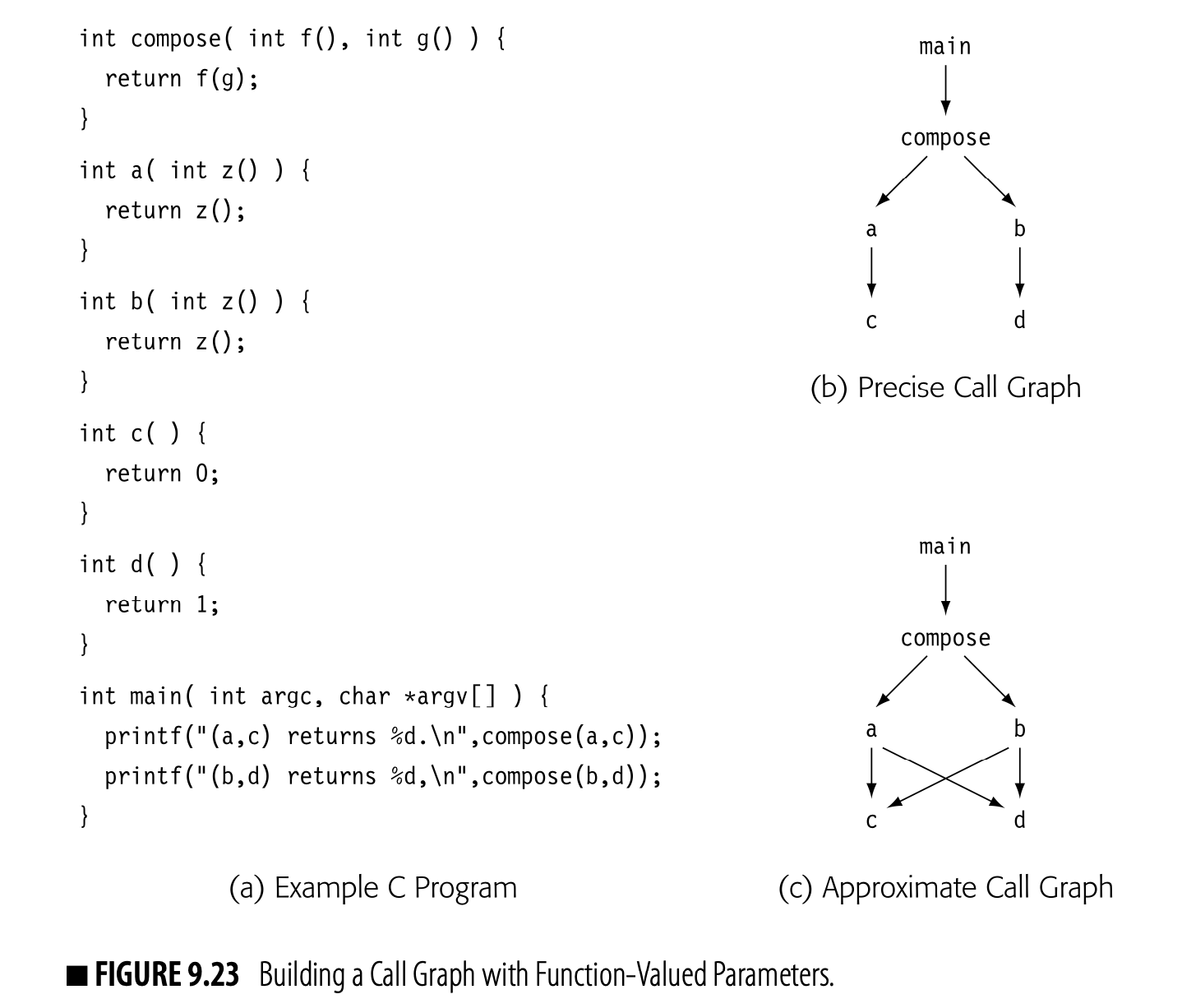
Source language features can complicate call-graph construction. For example, consider the small C program shown in Fig. 9.23(a). Its precise call graph is shown in panel (b). The following subsections outline the language features that complicate call-graph construction.

Procedure-Valued Variables

If the program uses procedure-valued variables, the compiler must either assume that a call to a procedure-valued variable can invoke any procedure, or it must analyze the program to estimate the set of possible callees at each such call site. To perform this analysis, the compiler can construct the graph specified by the calls that use explicit literal constants. Next, it can track the propagation of functions as values around this subset of the call graph, adding edges as indicated.

In SSCP, initialize any function-valued formal parameters with known constant values. Actual parameters with the known values reveal where functions are passed through.

The compiler can use a simple analog of global constant propagation to transfer function values from a procedure's entry to the call sites that use them, using set union as its meet operation.

Once it has a set of procedures that might be passed to a procedure-valued parameter, the compiler must model the transmission of that parameter to individual call sites in the procedure. Most programming languages do not allow operations on a procedure-value, so this modeling can be both simple and effective (see the discussion of jump functions in Section 9.4.2).

Fig. 9.23 shows that a straightforward analysis may overestimate the set of call-graph edges. The code calls compose to compute a(c) and b(d). A simple analysis, however, will conclude that the formal parameter g in compose can receive either c or d, and that, as a result, the program might compose any of a(c), a(d), b(c), or b(d), as shown in panel (c). To build the precise call graph, shown in panel (b), the compiler must track sets of parameters that are passed together, along the same path. The algorithm could then consider each set independently to derive the precise graph. Alternatively, it might tag each value with the path that the values travel and use the path information to avoid adding spurious edges such as (a,d) or (b,c).

Contextually Resolved Names

Some languages allow programmers to use names that are resolved by context. In object-oriented languages with an inheritance hierarchy, the binding of a method name to a specific implementation depends on the class of the receiver and the state of the inheritance hierarchy.

If the inheritance hierarchy and all the procedures are fixed at the time of analysis, then the compiler can use interprocedural analysis of the class structure to narrow the set of methods that can be invoked at any given call site. The call-graph constructor must include an edge from that call site to each procedure or method that might be invoked.

Dynamic linking, used in some operating systems to reduce virtual memory require- ments, introduces similar complications. If the compiler cannot determine what code will execute, it cannot construct a complete call graph.

For a language that allows the program to import either executable code or new class definitions at runtime, the compiler must construct a conservative call graph that reflects the complete set of potential callees at each call site. One option is to have the compiler construct a single call-graph node to represent these unknown procedures and to endow that node with worst-case behavior, such as maximal MayMod and MayRef sets. This strategy will ensure that other analyses have conservative approximations to the set of possible facts.

Analysis to resolve ambiguous calls can improve the precision of the call graph by reducing the number of spurious edges--edges for calls that cannot occur at runtime. Of equal or greater importance, any call site that can be resolved to a single callee can be implemented with a direct call; one with multiple callees may need a runtime lookup to dispatch the call (see Section 6.3.2). Runtime lookups to support dynamic dispatch can be much more expensive than a direct call.

Other Language Issues

In intraprocedural analysis, we assume that the control-flow graph has a single entry and a single exit; we add an artificial exit node if the procedure has multiple returns. The analogous problems arise in interprocedural analysis.

For example, JAVA has both initializers and finalizers. The JAVA virtual machine invokes a class initializer after it loads and verifies the class; it invokes an object initializer after it allocates space for the object but before it returns the object's hashcode. Thread start methods, finalizers, and destructors also have the property that they execute without an explicit call in the source program.

The call-graph builder must recognize and understand these procedures. It must connect them into the call graph in appropriate ways. The specific details will depend on the language definition and the analysis being performed. MayMod analysis, for example, might ignore them as irrelevant, while interprocedural constant propagation might need information from initialization and start methods.

9.4.2 Interprocedural Constant Propagation

Interprocedural constant propagation tracks known constant values of global variables and parameters as they propagate around the call graph, both through procedure bodies and across call-graph edges. The goal of interprocedural constant propagation is to discover places where a procedure always receives a known constant value or where a procedure always returns a known constant value. When the compiler finds such a constant, it can specialize the code to that value.

For the moment, we will restrict our attention to finding constant-valued formal parameters. The extension to global variables appears at the end of this section.

Conceptually, interprocedural constant propagation consists of three sub-problems: discovering an initial set of constants, propagating known constant values around the call graph, and modeling transmission of values through procedures.

Discovering an Initial Set of Constants

The analyzer must identify, at each call site, which actual parameters have known constant values. A wide range of techniques are possible. The simplest method is to recognize literal constant values used as parameters. A more effective and expensive approach could use global constant propagation (e.g., SSCP from Section 9.3.6) to identify constant-valued parameters.

Propagating Known Constant Values Around the Call Graph

Given an initial set of constants, the analyzer propagates the constant values across call-graph edges and through the procedures from entry to each call site in the procedure. This portion of the analysis resembles the iterative data-flow algorithms from Section 9.2. The iterative algorithm will solve this problem, but it may require significantly more iterations than it would for simpler problems such as live variables or available expressions.

Modeling Transmission of Values Through Procedures

Each time the analyzer processes a call-graph node, it must determine how the constant values known at the procedure's entry affect the set of constant values known at each of the call sites in the procedure. To do so, it builds a small model for each actual parameter, called a jump function. At a call site $s$ , we will denote the jump function for parameter $a$ as $J_{s}^{a}$ .

Each call site $s$ is represented with a vector of jump functions. If $s$ has $n$ parameters, the algorithm builds the vector $J_{s} = ⟨ J_{s}^{a}, J_{s}^{b}, J_{s}^{c}, \dots, J_{s}^{n} ⟩$ , where $a$ is the first formal parameter in the callee, $b$ is the second, and so on. Each jump function, $J_{s}^{x}$ , relies on the values of some subset of the global variables and the formal parameters to the procedure $p$ that contains $s$ ; we denote that set as Support( $J_{s}^{x}$ ).

For the moment, assume that $J_{s}^{x}$ consists of an expression tree whose leaves are all global variables, formal parameters of the caller, or literal constants. We require that $J_{s}^{x}$ return $⊤$ if Value(y) is $⊤$ for any $y \in Support (J_{s}^{x})$ .

The Algorithm

Fig. 9.24 shows a simple interprocedural constant propagation algorithm. It is similar to the SSCP algorithm presented in Section 9.3.6.

The algorithm associates a field Value( $x$ ) with each formal parameter $x$ of each procedure $p$ . (It assumes unique, or fully qualified, names for each formal parameter.) The first phase optimistically sets all the Value fields to $⊤$ . Next, it iterates over each actual parameter $a$ at each call site $s$ in the program, updates the Value field of $a$ 's corresponding formal parameter $f$ to $Value (f) \land J_{s}^{f}$ , and adds $f$ to the worklist. This step factors the initial set of constants represented by the jump functions into the $Value$ fields and sets the worklist to contain all of the formal parameters.

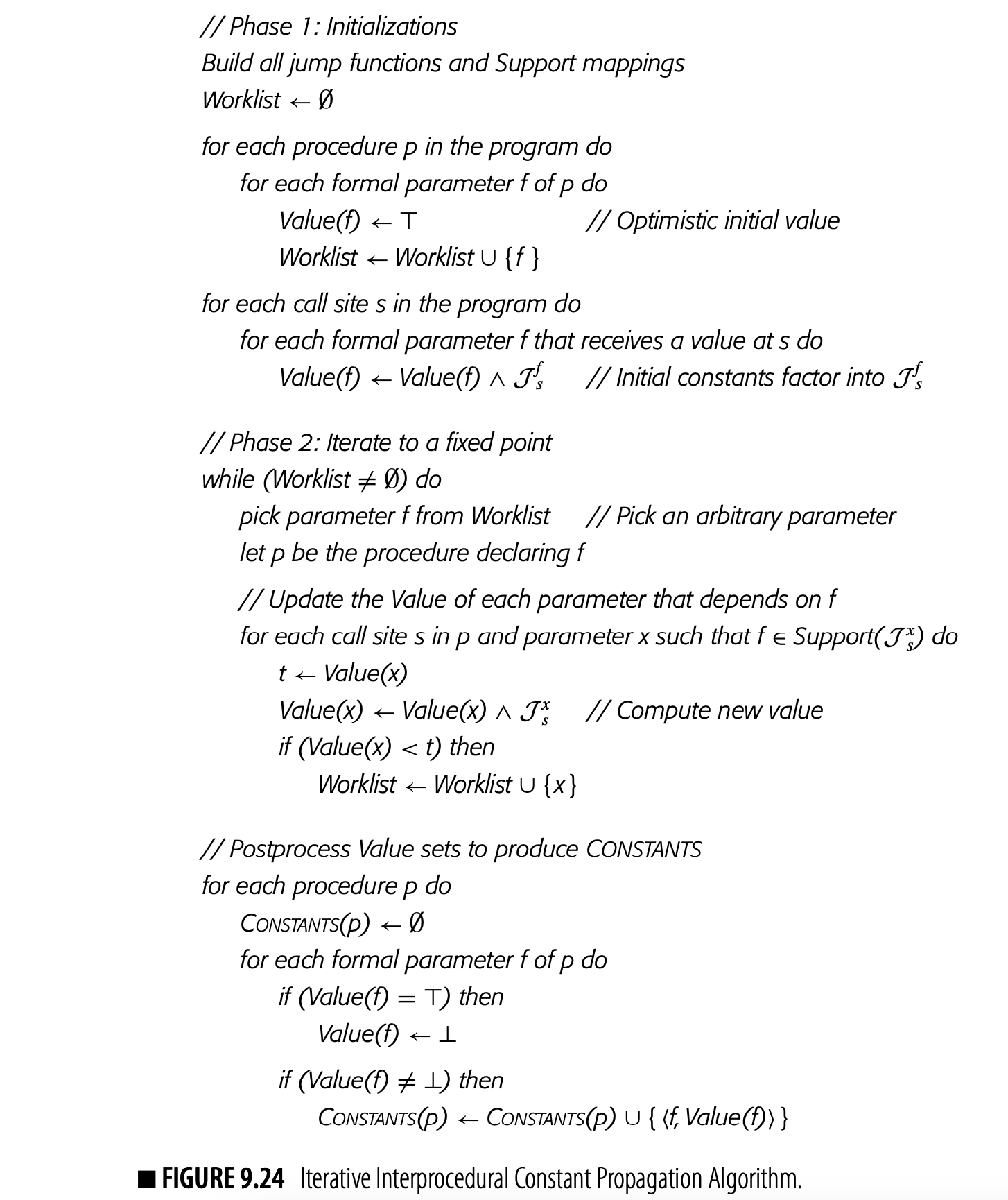
The second phase repeatedly selects a formal parameter from the worklist and propagates it. To propagate formal parameter $f$ of procedure $p$ , the analyzer finds each call site $s$ in $p$ and each formal parameter $x$ (which corresponds to an actual parameter of call site $s$ ) such that $f \in Support (J_{s}^{x})$ . It evaluates $J_{s}^{x}$ and combines it with $Value (x)$ . If $Value (x)$ changes, it adds $x$ to the worklist. The worklist should be implemented with a data structure, such as a sparse set, that does not allow duplicate members (see Section B.2.3).

This algorithm relies on the same semilattice-based termination argument used for SSCP in Section 9.3.6.

The second phase terminates because each Value set can take on at most three values in the semilattice: $⊤$ , some $c_{i}$ , and $⊥$ . A variable $x$ can only enter the worklist when its initial Value is computed or when its Value changes. Each variable $x$ can appear on the worklist at most three times. Thus, the total number of changes is bounded and the iteration halts. After the second phase halts, a postprocessing step constructs the sets of constants known on entry to each procedure.

Jump Function Implementation

For example, $Support (J_{s}^{x})$ might contain a value read from a file, so $J_{s}^{x} =⊥$ .

Implementations of jump functions range from simple static approximations that do not change during analysis, through small parameterized models, to more complex schemes that perform extensive analysis at each jump-function evaluation. In any of these schemes, several principles hold. If the analyzer determines that parameter $x$ at call site $s$ is a known constant $c$ , then $J_{s}^{x} = c$ and $Support (J_{s}^{x}) = \emptyset$ . If $y \in Support (J_{s}^{x})$ and $Value (y) = ⊤$ , then $J_{s}^{x} = ⊤$ . If the analyzer determines that the value of $J_{s}^{x}$ cannot be determined, then $J_{s}^{x} = ⊥$ .

The analyzer can implement $J_{s}^{x}$ in many ways. A simple implementation might only propagate a constant if the value enters the procedure as a formal parameter and passes, unchanged, to a parameter at a call site--that is, an actual parameter $x$ is the SSA name of a formal parameter in the procedure that contains call site $s$ . (Similar functionality can be obtained using Reaches information from Section 9.2.4.)

More complex schemes that find more constants are possible. The compiler could build expressions composed of SSA names of formal parameters and literal constants. The jump-function would then interpret the expression over the semilattice values of the SSA names and constants that it contains. To obtain even more precise results, the compiler could run the SSCP algorithm on demand to update the values of jump functions.

Extending the Algorithm

The algorithm shown in Fig. 9.24 only propagates constant-valued actual parameters forward along call-graph edges. We can extend it, in a natural way, to handle returned values and variables that are global to a procedure.

Just as the algorithm builds jump functions to model the flow of values from caller to callee, it can construct return jump functions to model the values returned from callee to caller. Return jump functions are particularly important for routines that initialize values, whether filling in a common block in FORTRAN or setting initial values for an object or class in JAVA. The algorithm can treat return jump functions in the same way that it handled ordinary jump functions; the one significant complication is that the implementation must avoid creating cycles of return jump functions that diverge (e.g., for a tail-recursive procedure).

To extend the algorithm to cover a larger class of variables, the compiler can extend the vector of jump functions in an appropriate way. Expanding the set of variables will increase the cost of analysis, but two factors mitigate the cost. First, in jump-function construction, the analyzer can notice that many of those variables do not have a value that can be modeled easily; it can map those variables onto a universal jump function that returns $⊥$ and avoid placing them on the worklist. Second, for the variables that might have constant values, the structure of the lattice ensures that they will be on the worklist at most twice. Thus, the algorithm should still run quickly.

Section Review

Compilers perform interprocedural analysis to capture the behavior of all the procedures in the program and to bring that knowledge to bear on optimization within individual procedures. To perform interprocedural analysis, the compiler must model all of the code that it analyzes. A typical interprocedural problem requires the compiler to build a call graph (or some analog), to annotate it with information derived directly from the individual procedures, and to propagate that information around the graph.

The results of interprocedural information are applied directly in intraprocedural analysis and optimization. For example, MarMood and MarRer sets can be used to mitigate the impact of a call site on global data-flow analyses or to avoid the necessity for $ϕ$ -functions after a call site. The results of interprocedural constant propagation can be used to initialize a global algorithm, such as sparse conditional constant propagation (see Section 0.1.7).

Review Questions

Call-graph construction has many similarities to interprocedural constant propagation. The call-graph algorithm can achieve good results with relatively simple jump functions. What features could a language designer add that might necessitate more complex jump functions in the call-graph constructor?
How might the analyzer incorporate MarMood information into interprocedural constant propagation? What effect would you expect it to have?

9.5 Advanced Topics

Section 9.2 focused on iterative data-flow analysis. It emphasized the iterative approach because it is simple, robust, and efficient. Other approaches to data-flow analysis tend to rely heavily on structural properties of the underlying graph. Section 9.5 discusses flow-graph reducibility--a critical property for most of the structural algorithms.

Section 9.5.2 revisits the iterative dominance framework from Section 9.2.1. The simplicity of that framework makes it attractive; however, more specialized and complex algorithms have significantly lower asymptotic complexities. In Section 9.5.2, we introduce a set of data structures that make the simple iterative technique competitive with the fast dominator algorithms for flow graphs of up to several thousand nodes.

9.5.1 Structural Data-Flow Analysis and Reducibility

Chapters 8 and 9 present an iterative formulation of data-flow analysis. The iterative algorithm works, in general, on any set of well-formed equations on any graph. Other data-flow algorithms exist; many of these work by deriving a simple model of the control-flow structure of the code being analyzed and using that model to solve the equations. Often, that model is built by finding a sequence of transformations to the CFG that reduce its complexity--by combining nodes or edges in carefully defined ways. This graph-reduction process lies at the heart of almost every data-flow algorithm except the iterative algorithm.

Reducible graph A flow graph is reducible if the two transformations, $T_{1}$ and $T_{2}$ , will reduce it to a single node. If that process fails, the graph is $irreducible$ .

These $s t r u c t u r a l$ data-flow algorithms use a small set of transformations, each of which selects a subgraph and replaces it by a single node to represent the subgraph. This creates a series of derived graphs in which each graph differs from its predecessor in the series by the effect of applying a single transformation. As the analyzer transforms the graph, it computes data-flow sets for the new representer nodes in each successive derived graph. These sets summarize the replaced subgraph's effects. The transformations reduce well-behaved graphs to a single node. The algorithm then reverses the process, going from the final derived graph, with its single node, back to the original flow graph. As it expands the graph back to its original form, the analyzer computes the final data-flow sets for each node.

In essence, the reduction phase gathers information from the entire graph and consolidates it, while the expansion phase propagates the effects in the consolidated set back out to the nodes of the original graph. Any graph for which such a reduction sequence succeeds is deemed reducible. If the graph cannot be reduced to a single node, it is irreducible. 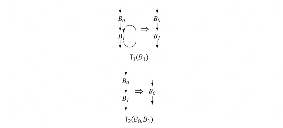To demonstrate reducibility, we can use the two graph transformations, called $T_{1}$ and $T_{2}$ , shown in the margin. These same transformations form the basis for a classic data-flow algorithm. $T_{1}$ removes a self loop, which is an edge that runs from a node back to itself. The drawing in the margin shows $T_{1}$ applied to $B_{I}$ , denoted $T_{1} (B_{I})$ . $T_{2}$ folds a node $B_{I}$ that has exactly one predecessor $B_{0}$ back into $B_{0}$ ; it removes the edge $⟨ B_{0}, B_{I} ⟩$ , and makes $B_{0}$ the source of any edges that originally left $B_{I}$ . If this leaves multiple edges from $B_{0}$ to some other node $n$ , it consolidates those edges. The drawing in the margin shows $T_{2} (B_{0}, B_{I})$ .

Any graph that can be transformed, or reduced, to a single node by repeated application of $T_{1}$ and $T_{2}$ is deemed reducible. To understand how this works, consider the CFG from our continuing example. Fig. 9.25(a) shows one sequence of applications of $T_{1}$ and $T_{2}$ that reduces the CFG to a single-node graph. The sequence applies $T_{2}$ until no more opportunities exist: $T_{2} (B_{I}, B_{2})$ , $T_{2} (B_{5}, B_{6})$ , $T_{2} (B_{5}, B_{8})$ , $T_{2} (B_{5}, B_{7})$ , $T_{2} (B_{I}, B_{5})$ , and $T_{2} (B_{I}, B_{3})$ . Next, it uses $T_{1} (B_{I})$ to remove the loop. Finally, it applies $T_{2} (B_{0}, B_{I})$ and $T_{2} (B_{0}, B_{4})$ to reduce the graph to a single node. This sequence proves that the graph is reducible.

Other application orders also reduce the graph. For example, starting with $T_{2} (B_{I}, B_{3})$ leads to a different transformation sequence. $T_{1}$ and $T_{2}$ have the finite Church-Rosser property, which ensures that the final result is independent of the order of application and that the sequence terminates. Thus, the analyzer can find places in the graph where $T_{1}$ or $T_{2}$ applies and use them opportunistically.

Fig. 9.25(b) shows what can happen when we apply $T_{1}$ and $T_{2}$ to a graph with multiple-entry loops. The analyzer uses $T_{2} (B_{0}, B_{I})$ followed by $T_{2} (B_{0}, B_{5})$ . At that point, however, no remaining node or pair of nodes is a candidate for either $T_{1}$ or $T_{2}$ . Thus, the analyzer cannot reduce the graph any further. (No other order will work either.) The graph cannot be reduced to a single node; it is irreducible.

Many other tests for graph reducibility exist. One fast and simple test is to apply the iterative DOM framework to the graph, using an RPO traversal order. If the calculation needs more than two iterations over a graph, that graph is irreducible.

The failure of $T_{1}$ and $T_{2}$ to reduce this graph arises from a fundamental property of the graph. The graph is irreducible because it contains a loop, or cycle, that has edges that enter it at different nodes. In terms of the source language, the program that generated the graph has a loop with multiple entries. We can see this property in the graph; consider the cycle formed by $B_{2}$ and $B_{3}$ . It has edges entering it from $B_{I}$ , $B_{4}$ , and $B_{5}$ . Similarly, the cycle formed by $B_{3}$ and $B_{4}$ has edges that enter it from $B_{2}$ and $B_{5}$ .

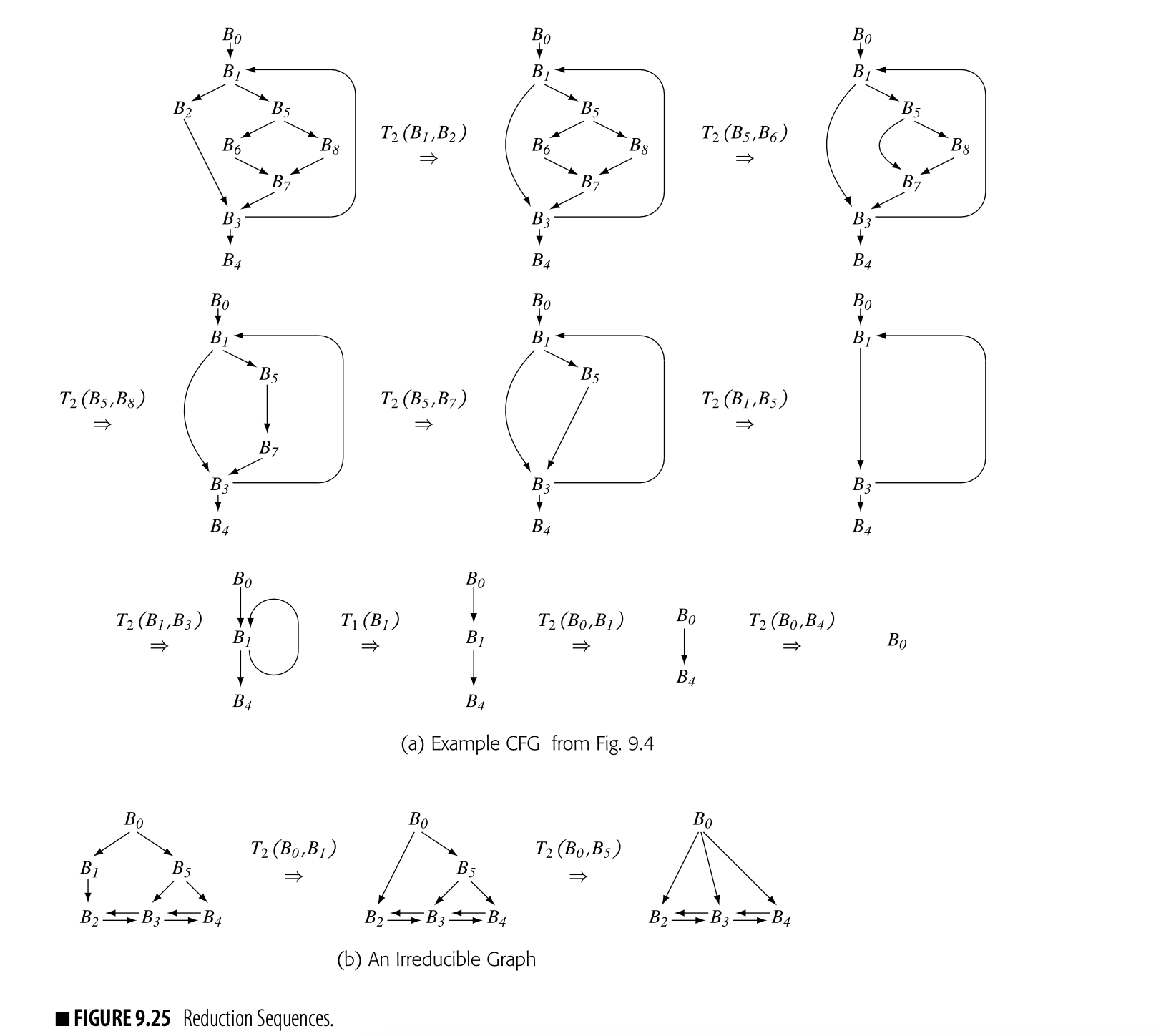
Irreducibility poses a serious problem for algorithms built on transformations like $T_{1}$ and $T_{2}$ . If the algorithm cannot reduce the graph to a single-node, then the method must either report failure, modify the graph by splitting one or more nodes, or use an iterative approach to solve the system on the partially reduced graph. In general, structural algorithms for data-flow analysis only work on reducible graphs. The iterative algorithm, by contrast, works correctly, albeit more slowly, on an irreducible graph. 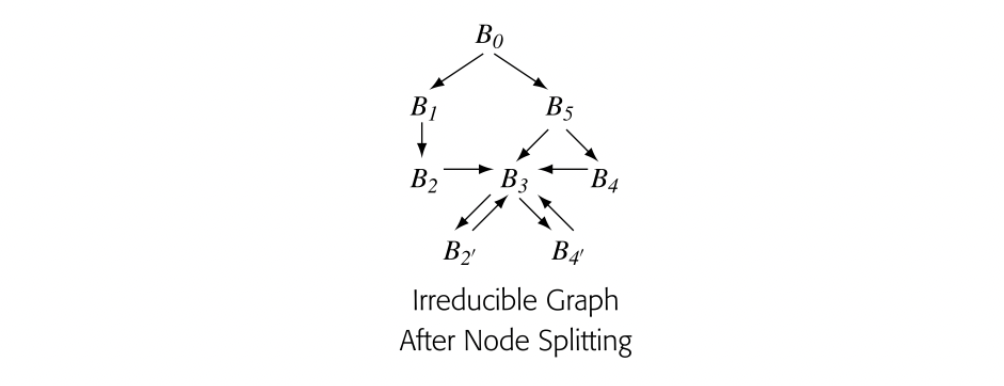To transform an irreducible graph to a reducible graph, the analyzer can split one or more nodes. The simplest split for the example graph from Fig. 9.25(b) is shown in the margin. The transformation has cloned $B_{2}$ and $B_{d}$ to create $B_{2^{'}}$ and $B_{d^{'}}$ , respectively. The analyzer then retargets the edges $(B_{3}, B_{2})$ and $(B_{3}, B_{4})$ to form a complex loop, ${B_{3}, B_{2^{'}}, B_{4^{'}}}$ . The new loop has a single entry, through $B_{3}$ .

This transformation creates a reducible graph that executes the same sequence of operations as the original graph. Paths that, in the original graph, entered $B_{3}$ from either $B_{2}$ or $B_{4}$ now execute as prologs to the loop ${B_{3}, B_{2^{'}}, B_{4^{'}}}$ . Both $B_{2}$ and $B_{4}$ have unique predecessors in the new graph. $B_{3}$ has multiple predecessors, but it is the sole entry to the loop and the loop is reducible. Thus, node splitting produced a reducible graph, at the cost of cloning two nodes.

In the reverse CFG, the break becomes a second entry to the cyclic region.

Both folklore and published studies suggest that irreducible graphs rarely arise in global data-flow analysis. The rise of structured programming in the 1970s made programmers much less likely to use arbitrary transfers of control, like a goto statement. Structured loop constructs, such as do, for, while, and until loops, cannot produce irreducible graphs. However, transferring control out of a loop (for example, C's break statement) creates a CFG that is irreducible to a backward analysis. Similarly, irreducible graphs may arise more often in interprocedural analysis due to mutually recursive subroutines. For example, the call graph of a recursive-descent parser is likely to have irreducible subgraphs. Fortunately, an iterative analyzer can handle irreducible graphs correctly and efficiently.

A simple way to avoid worst case behavior from an irreducible graph in an iterative analyzer is to compute two traversal orders, one based on the treewalk that traverses siblings left-to-right and another based on a right-to-left traversal. Alternating between these two orders on successive passes will improve behavior on worst-case irreducible graphs.

9.5.2 Speeding up the Iterative Dominance Framework

The iterative framework for computing dominance is particularly simple. Where most data-flow problems have equations involving several sets, the equations for Dom involve computing a pairwise intersection over Dom sets and adding a single element to those sets. The simple nature of these equations presents an opportunity; we can use a sparse data-structure to improve the speed of the $Dom$ calculation.

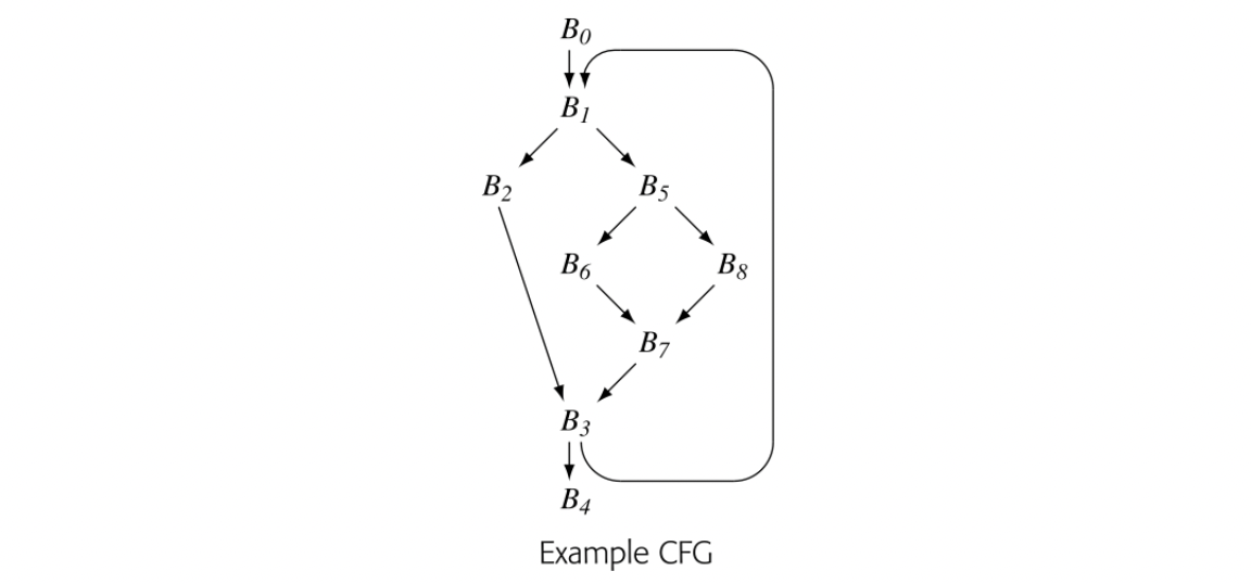
The iterative Dom framework described in Section 9.2.1 stores a full Dom set at each node. The compiler can achieve the same result by storing just the immediate dominator, or IDom, at each node and solving for IDom. The compiler can easily recreate Dom( $n$ ) when needed. Since IDom is a singleton set, the implementation can be quite efficient.

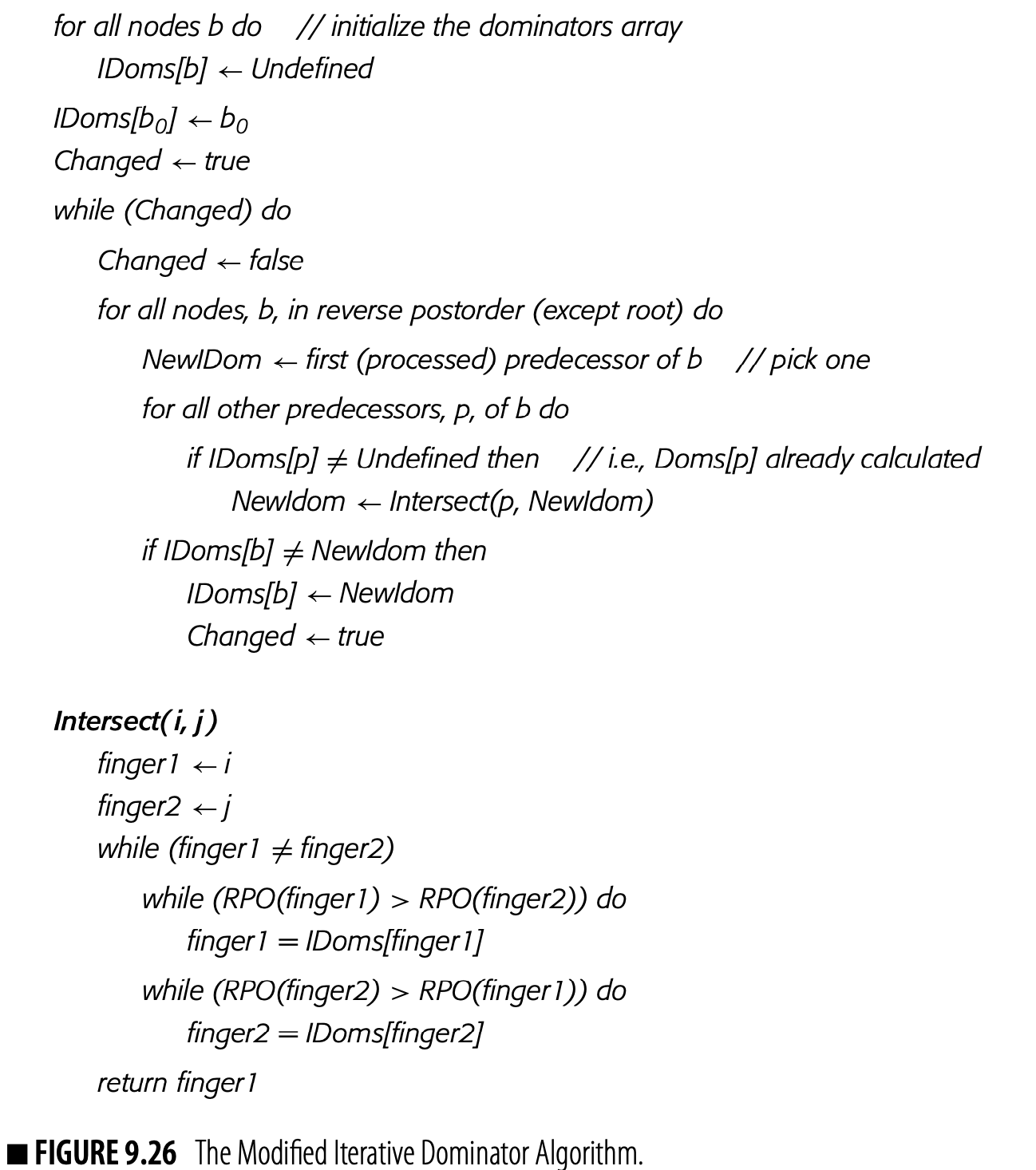
Recall our example CFG from Section 9.2.1, repeated in the margins along with its dominator tree. Its IDom sets are as follows:

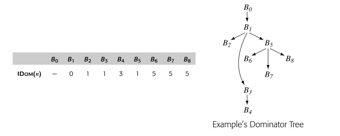
Notice that the dominator tree and the IDoms are isomorphic. IDom( $b$ ) is just $b$ 's predecessor in the dominator tree. The root of the dominator tree has no predecessor; accordingly, its IDom set is undefined.

The compiler can read a graph's Dom sets from its dominator tree. For a node $n$ , its Dom set is just the set of nodes that lie on the path from $n$ to the root of the dominator tree, inclusive of the end points. In the example, the dominator-tree path from $B_{7}$ to $B_{0}$ consists of $(B_{7}, B_{5}, B_{1}, B_{0})$ , which matches Dom( $B_{7}$ ) from Section 9.2.1.

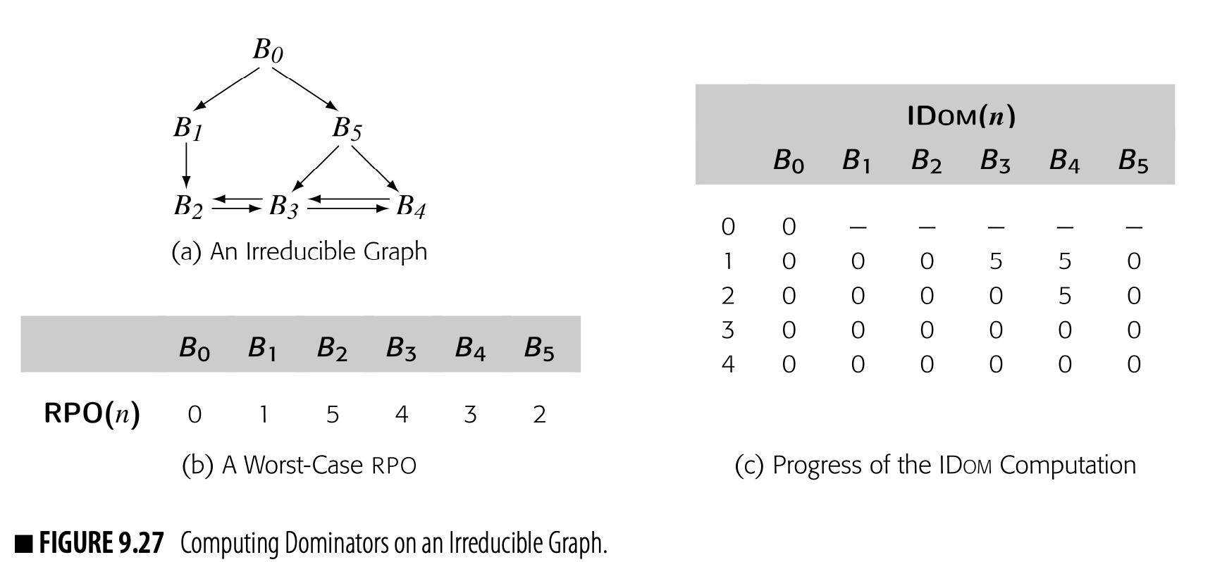
Thus, the compiler can use the IDom sets as a proxy for the Dom sets, provided that it can initialize and intersect the sets efficiently. A small modification to the iterative algorithm can simplify initialization. Intersection requires a more subtle approach, shown in Fig. 9.26. The critical procedure, intersect, relies on two observations:

When the algorithm walks the path from a node to the root to recreate a Dom set, it encounters the nodes in a consistent order. The intersection of two Dom sets is simply the common suffix of the labels on the paths from the nodes to the root.
The algorithm needs to recognize the common suffix. It starts at the two nodes whose sets are being intersected, $i$ and $j$ , and walks upward in the dominator tree from each of them toward the root. If we name the nodes by their RPO numbers, then a simple comparison will let the algorithm discover the nearest common ancestor--the IDom of $i$ and $j$ .

intersect is a variant of the classic "two finger" algorithm. It uses two pointers to trace paths upward through the tree. When they agree, they both point to the node representing the result of the intersection.

Fig. 9.26 shows a reformulated iterative algorithm for IDom. It keeps the IDom information in an array, IDoms. It initializes the IDom entry for the root, b $_{0}$ , to itself to simplify the rest of the algorithm. It processes the nodes in reverse postorder. In computing intersections, it ignores predecessors whose IDoms have not yet been computed.

To see how the algorithm operates, consider the irreducible graph in Fig. 9.27(a). Panel (b) shows an RPO for this graph that illustrates the problems caused by irreducibility. Using this order, the algorithm miscomputes the IDoms of $B_{3}$ , and $B_{4}$ in the first iteration. It takes two iterations for thealgorithm to correct those IDoms, and a final iteration to recognize that the IDoms have stopped changing.

This improved algorithm runs quickly. It has a small memory footprint. On any reducible graph, it halts in two passes: the first pass computes the correct IDom sets and the second pass confirms that no changes occur. An irreducible graph will take more than two passes. In fact, the algorithm provides a rapid test for reducibility--if any IDom entry changes in the second pass, the graph is irreducible.

9.6 Summary and Perspective

Most optimization tailors general-case code to the specific context that occurs in the compiled code. The compiler's ability to tailor code is often limited by its lack of knowledge about the program's range of runtime behaviors.

Data-flow analysis allows the compiler to model the runtime behavior of a program at compile time and to draw important, specific knowledge from these models. Many data-flow problems have been proposed; this chapter presented several of them. Many of those problems have properties that lead to efficient analyses.

SSA form is both an intermediate form and a tool for analysis. It encodes both data-flow information and control-dependence information into the name space of the program. Using SSA form as the basis for an algorithm has three potential benefits. It can lead to more precise analysis, because SSA incorporates control-flow information. It can lead to more efficient algorithms, because SSA is a sparse representation for the underlying data-flow information. It can lead to simpler formulations of the underlying optimization (see Section 10.7.2). These advantages have led both researchers and practitioners to adopt SSA form as a definitive representation in modern compilers.

Chapter Notes

Credit for the first data-flow analysis is usually given to Vyssotsky at Bell Labs in the early 1960s [351]. Lois Haibt's work, in the original FORTRAN compiler, predates Vyssotsky. Her phase of the compiler built a control-flow graph and performed a Markov-style analysis over the CFG to estimate execution frequencies [27].

Iterative data-flow analysis has a long history in the literature. Among the seminal papers on this topic are Kildall's 1973 paper [234], work by Hechtand Ullman [197], and two papers by Kam and Ullman [221, 222]. The treatment in this chapter follows Kam & Ullman.

This chapter focuses on iterative data-flow analysis. Many other algorithms for solving data-flow problems have been proposed [229]. The interested reader should explore the structural techniques, including interval analysis [18, 19, 68]; $T_{1}$ - $T_{2}$ analysis [196, 348]; the Graham-Wegman algorithm [178, 179]; the balanced-tree, path-compression algorithm [342, 343]; graph grammars [230]; and the partitioned-variable technique [371]. The alternating-direction iterative method mentioned at the end of Section 9.5.1 is due to Harvey [109].

Dominance has a long history in the literature. Prosser introduced dominance in 1959 but gave no algorithm to compute dominators [300]. Lowry and Medlock describe the algorithm used in their compiler [260]; it takes at least \mathsf{O}\big{(}N^{2}\big{)} time, where $N$ is the number of statements in the procedure. Several authors developed faster algorithms based on removing nodes from the cfg[4, 9, 301]. Tarjan proposed an $O (N lo g N + E)$ algorithm based on depth-first search and union find [341]. Lengauer and Tarjan improved this time bound [252], as did others [24, 67, 190]. The data-flow formulation for dominators is taken from Allen [13, 18]. The fast data structures for iterative dominance are due to Harvey [110]. The algorithm in Fig. 9.10 is from Ferrante, Ottenstein, and Warren [155].

The SSA construction is based on the seminal work by Cytron et al. [120]. That work builds on work by Shapiro and Saint [323]; by Reif [305, 344]; and by Ferrante, Ottenstein, and Warren [155]. The algorithm in Section 9.3.3 builds semipruned SSA[55]. Briggs et al. describe the details of the renaming algorithm and the ad-hoc approach to out-of-SSA translation [56]. The unified approach to out-of-SSA translation is due to Boissinot et al. [51]. The complications introduced by critical edges have long been recognized in the literature of optimization [139, 141, 142, 236, 312]; it should not be surprising that they also arise in the translation from SSA back into executable code. The sparse simple constant algorithm, SSCP, is due to Reif and Lewis [306]. Wegman and Zadeck reformulate SSCP to use SSA form [358, 359].

The IBM PL/I optimizing compiler was one of the earliest systems to perform interprocedural data-flow analysis [334]. Call-graph construction is heavily language dependent: Ryder looked at the problems that arise in Fortran [314], C [272], and JAVA[372]. Shivers wrote the classic paper on control-flow analysis in Scheme-like languages [325].

Early work on side-effect analysis focused more on defining the problems than on their fast solution [35, 37]. Cooper and Kennedy developed simple frameworks for MayMod and MayRef that led to fast algorithms for these problems [112, 113]. The interprocedural constant propagation algorithm is from Torczon's thesis and subsequent papers [74, 182, 271]; both Cytron and Wegman suggested other approaches to the problem [121, 359]. Burke and Torczon [70] formulated an analysis that determines which modules in a large program must be recompiled in response to a change in a program's interprocedural information. Pointer analysis is inherently interprocedural; a growing body of literature describes that problem [84, 87, 123, 134, 149, 202, 203, 209, 247, 322, 360, 363]. Ayers, Gottlieb, and Schooler described a practical system that analyzed and optimized a subset of the entire program [26].

Exercises

In live analysis, the equations initialize the LiveOut set of each block to $\emptyset$ . Are other initializations possible? Do they change the result of the analysis? Justify your answer.
In live analysis, how should the compiler treat a block containing a procedure call? What should the block's UEVar set contain? What should its VarKill set contain?
For each of the following control-flow graphs: a. Compute reverse postorder numberings for the CFG and the reverse CFG. b. Compute reverse preorder on the CFG. c. Is reverse preorder on the CFG equivalent to postorder on the reverse CFG?
- Consider the three control-flow graphs shown in Fig. 9.28.
- Compute the dominator trees for CFGs (a), (b), and (c).
- Compute the dominance frontiers for nodes 3 and 5 of (a), nodes 4 and 5 of (b), and nodes 2 and 10 of (c).
- Translate the code in the cfg shown below into SSA form. Show only the final results, after both $ϕ$ -insertion and renaming.
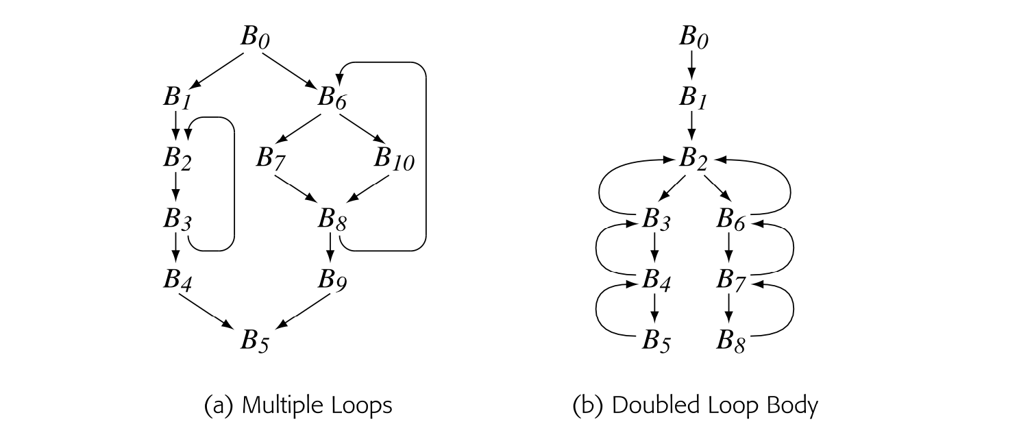
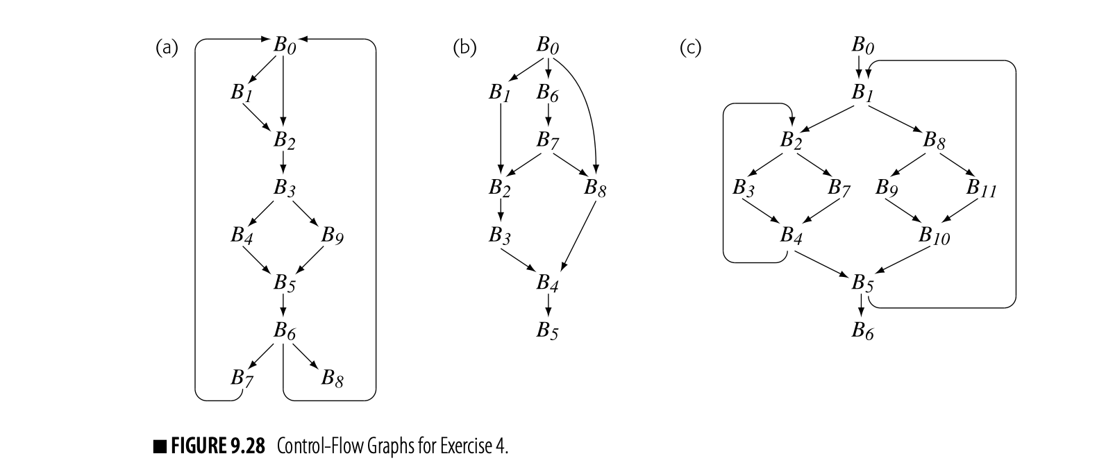
Consider the three control-flow graphs shown in Fig. 9.28.
1. Compute the dominator trees for CFGs (a), (b), and (c).
2. Compute the dominance frontiers for nodes 3 and 5 of (a), nodes 4 and 5 of (b), and nodes 2 and 10 of (c).
Translate the code in the CFG shown below into SSA form. Show only the final results, after both φ-insertion and renaming.
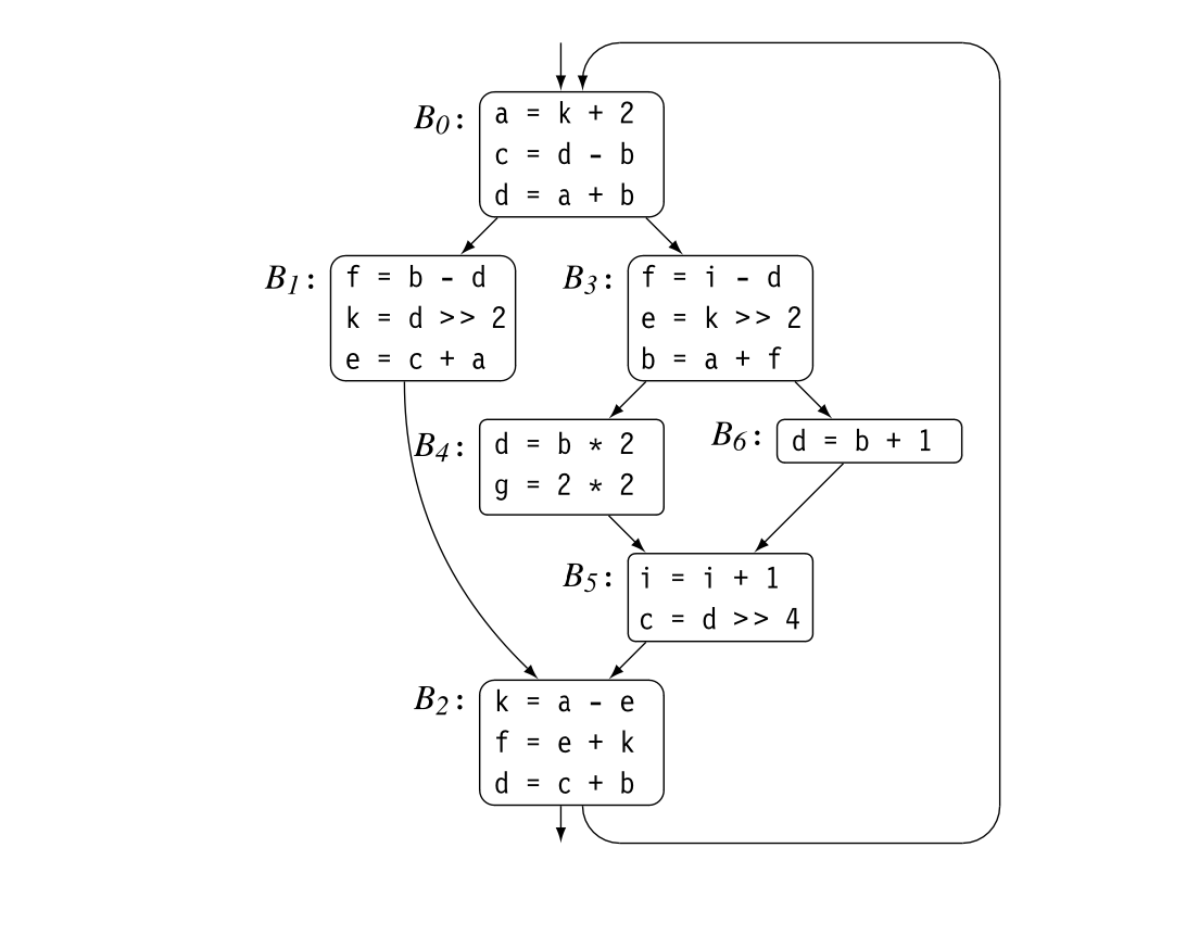
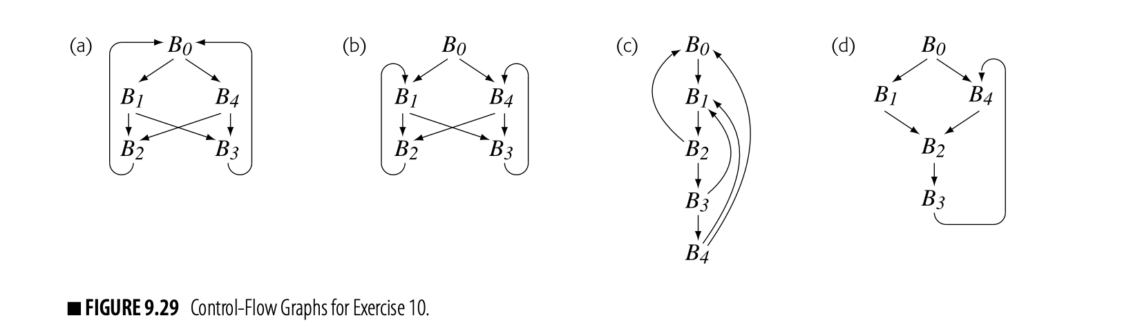
Given an assignment to some variable $v$ in block $b$ , consider the set of blocks that need a $ϕ$ -function as a result. The algorithm in Fig. 9.11 inserts a $ϕ$ -function in each block in $DF (b)$ . It then adds each of those blocks to the worklist; they, in turn, may add more blocks to the worklist. Call the set of all these blocks $DF^{+} (b)$ . We can define $DF^{+} (b)$ as the limit of the sequence: 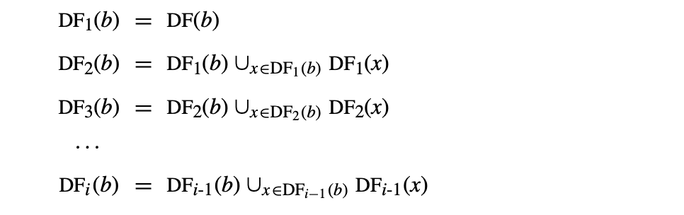Using these extended sets, $DF^{+} (b)$ , leads to a simpler algorithm for inserting $ϕ$ -functions. a. Develop an algorithm to compute $DF^{+} (b)$ . b. Develop an algorithm to insert $ϕ$ -functions using the $DF^{+}$ sets computed in part (a). c. Compare the overall cost of your algorithm, including the computation of $DF^{+}$ sets, to the cost of the $ϕ$ -insertion algorithm given in Section 9.3.3.
The maximal SSA construction is both simple and intuitive. However, it can insert many more $ϕ$ -functions than the semipruned algorithm. In particular, it can insert both redundant $ϕ$ -functions ( $x_{1} \leftarrow ϕ (x_{j}, x_{j})$ ) and dead $ϕ$ -functions--functions whose results are never used. a. Propose a method to detect and remove the extra $ϕ$ -functions that the maximal construction inserts. b. Can your method reduce the set of $ϕ$ -functions to just those that the semipruned construction inserts? c. Contrast the asymptotic complexity of your method against that of the semipruned construction.
Apply the unified out-of-SSA translation scheme to the example code for the lost-copy problem, shown in Fig. 9.18(a).
Apply the unified out-of-SSA translation scheme to the example code for the swap problem, shown in Fig. 9.19(a).
For each of the control-flow graphs shown in Fig. 9.29, show whether or not it is reducible. (Hint: use a sequence of $T_{1}$ and $T_{2}$ to show that the graph is reducible. If no such sequence exists, it is irreducible.)
Prove that the following definition of a reducible graph is equivalent to the definition that uses the transformations $T_{1}$ and $T_{2}$ : "A graph $G$ is reducible if and only if for each cycle in $G$ , there exists a node $n$ in the cycle with the property that $n$ dominates every node in that cycle."

13 Register Allocation

ABSTRACT

The code generated by a compiler must make effective use of the limited resources of the target processor. Among the most constrained resources is the set of hardware registers. Register use plays a major role in determining the performance of compiled code. At the same time, register allocation--the process of deciding which values to keep in registers--is a combinatorially hard problem.

Most compilers decouple decisions about register allocation from other optimization decisions. Thus, most compilers include a separate pass for register allocation. This chapter begins with local register allocation, as a way to introduce the problem and the terminology. The bulk of the chapter focuses on global register allocation and assignment via graph coloring. The advanced topics section discusses some of the many variations on that technique that have been explored in research and employed in practice.

Keywords

13.1 Introduction

Registers are a prominent feature of most processor architectures. Because the processor can access registers faster than it can access memory, register use plays an important role in the runtime performance of compiled code. Register allocation is sufficiently complex that most compilers implement it as a separate pass, either before or after instruction scheduling.

The register allocator determines, at each point in the code, which values will reside in registers and which will reside in memory. Once that decision is made, the allocator must rewrite the code to enforce it, which typically adds load and store operations to move values between memory and specific registers. The allocator might relegate a value to memory because the code contains more live values than the target machine's register set can hold. Alternatively, the allocator might keep a value in memory between uses because it cannot prove that the value can safely reside in a register.

Conceptual Roadmap

A compiler's register allocator takes as input a program that uses some arbitrary number of registers. The allocator transforms the code into an equivalent program that fits into the finite register set of the target machine. It decides, at each point in the code, which values will reside in registers and which will reside in memory. In general, accessing data in registers is faster than accessing it in memory.

Spill When the allocator moves a value from a register to memory, it is said to spill the value.

To transform the code so that it fits into the target machine's register set, the allocator inserts load and store operations that move values, as needed, between registers and memory. These added operations, or "spill code," include loads, stores, and address computations. The allocator tries to minimize the runtime costs of these spills and restores.

Restore When the allocator retrieves a previously spilled value, it is said to restore the value.

As a final complication, register allocation is combinatorially hard. The problems that underlie allocation and assignment are, in their most general forms, NP-complete. Thus, the allocator cannot guarantee optimal solutions in any reasonable amount of time. A good register allocator runs quickly--somewhere between $O (n)$ and $O (n^{2})$ time, where $n$ is the size of the input program. Thus, a good register allocator computes an effective approximate solution to a hard problem, and does it quickly.

Few Words About Time

The register allocator runs at compile time to rewrite the almost-translated program from the IR program's name space into the actual registers and memory of the target ISA. Register allocation may be followed by a scheduling pass or a final optimization, such as a peephole optimization pass.

The allocator produces code that executes at runtime. Thus, when the allocator reasons about the cost of various decisions, it makes a compile-time estimate of the expected change in running time of the final code. These estimates are, of necessity, approximations.

A few compiler systems have included description-driven, retargetable register allocators. To reconfigure these systems, the compiler writer builds a description of the target machine at design time; build-time tools then construct a working allocator.

Overview

Virtual register a symbolic register name that the compiler uses, before register allocation We write virtual registers as $V R_{i}$ , for $i \geq 0$

To simplify the earlier phases of translation, many compilers use an IR in which the name space is not tied to either the address space of the target processor or its register set. To translate the IR code into assembly code for the target machine, these names must be mapped onto the hardware resourcesof the target machine. Values stored in memory in the IR program must be turned into runtime addresses, using techniques such as those described in Section 7.3. Values kept in virtual registers (VRs) must be mapped into the processor's physical registers (PRs).

Physical register an actual register on the target processor We write physical registers as $P R_{i}$ , for $i \geq 0$ .

The underlying memory model of the IR program determines, to a large extent, the register allocator's role (see Section 4.7.1).

With a register-to-register memory model, the IR uses as many VRs as needed without regard for the size of the PR set. The register allocator must then map the set of VRs onto the set of PRs and insert code to move values between PRs and memory as needed.
With a memory-to-memory model, the IR keeps all program values in memory, except in the immediate neighborhood of an operation that defines or uses the value. The register allocator can promote a value from memory to a register for a portion of its lifetime to improve performance.

Thus, in a register-to-register model, the input code may not be in a form where it could actually execute on the target computer. The register allocator rewrites that code into a name space and a form where it can execute on the target machine. In the process, the allocator tries to minimize the cost of the new code that it inserts. By contrast, in a memory-to-memory model, all of the data motion between registers and memory is explicit; the code could execute on the target machine. In this situation, allocation becomes an optimization that tries to keep some values in registers longer than the input code did.

Graph coloring an assignment of colors to the nodes of a graph so that two nodes, $n 1$ and $n 2$ , have different colors if the graph contains the edge $(n 1, n 2)$ .

This chapter focuses on global register allocation in a compiler with a register-to-register memory model. Section 13.3 examines the issues that arise in a single-block allocator; that local allocator, in turn, helps to motivate the need for global allocation. Section 13.4 explores global register allocation via graph coloring. Finally, Section 13.5 explores variations on the global coloring scheme that have been discussed in the literature and tried in practical compilers.

13.2 Background

The design and implementation of a register allocator is a complex task. The decisions made in allocator design may depend on decisions made earlier in the compiler. At the same time, design decisions for the allocator may dictate decisions in earlier passes of the compiler. This section introduces some of the issues that arise in allocator design.

13.2.1 A Name Space for Allocation: Live Ranges

At its heart, the register allocator creates a new name space for the code. It receives code written in terms of Vrs and memory locations; it rewrites the code in a way that maps those Vrs onto both the physical registers and some additional memory locations.

To improve the efficiency of the generated code, the allocator should minimize unneeded data movement, both between registers and memory, and among registers. If the allocator decides to keep some value $x$ in a physical register, it should arrange, if possible, for each definition of $x$ to target the same PR and for each use of $x$ to read that PR. This goal, if achieved, eliminates unneeded register-to-register copy operations; it may also eliminate some stores and loads.

Live range a closed set of related definitions and uses Most allocators use live ranges as values that they consider for placement in a physi- cal register or in memory.

Most register allocators construct a new name space: a name space of live ranges. Each live range (LR) corresponds to a single value, within the scope that the allocator examines. The allocator analyzes the flow of values in the code, constructs its set of LRs, and renames the code to use LR names. The details of what constitutes an LR differ across the scope of allocation and between different allocation algorithms.

In a single block, LRs are easy to visualize and understand. Each LR corresponds to a single definition and extends from that definition to the value's last use. Fig. 13.1(a) shows an ILOC fragment that appeared in Chapter 1; panel (b) shows the code renamed into its distinct live ranges. The live ranges are shown as a graph in panel (c). The graph can be summarized as a set of intervals; for example LR $_{2}$ is [6, 9] and LR $_{8}$ is [3, 6]. The drawing in panel (c) assumes no overlap between execution of the operations.

We denote LR $_{8}$ as starting in operation three because the operation reads its arguments at the start of its execution and writes its result at the end of its execution. Thus, LR $_{8}$ is actually defined at the end of the second operation. By convention, we mark a live range as starting with the first operation after it has been defined. This treatment makes clear that the two instances of $r_{1}$ in addI $r_{1}$ , $10 \Rightarrow r_{1}$ are not the same live range, unless other context makes them so.

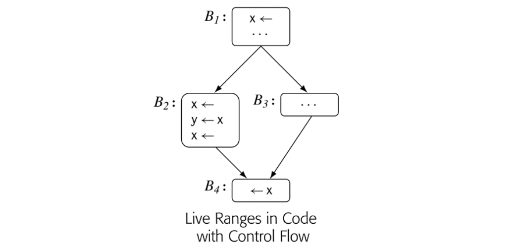
An LR ends for one of two reasons. An operation may be the name's last use along the current path through the code. Alternatively, the code might redefine the name before its next use, to start a new LR.

In a CFG with control flow, the situation is more complex, as shown in the margin. Consider the variable x. Its three definitions form two separate and distinct live ranges.

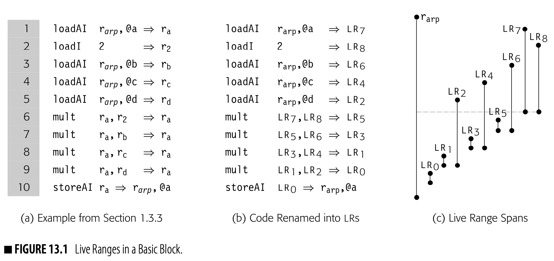
The use in $B_{4}$ refers to two definitions: the one in $B_{1}$ and the one at the bottom of $B_{2}$ . These three events create the first LR, denoted LR1. LR1 spans $B_{1}$ , $B_{3}$ , $B_{4}$ , and the last statement in $B_{2}$ .
The use of x in $B_{2}$ refers only to the definition that precedes it in $B_{2}$ . This pair creates a second LR, denoted LR2. LR1 and LR2 are independent of each other.

With more complex control flow, live ranges can take on more complicated shapes. In the global allocator from Section 13.4, an LR consists of all the definitions that reach some use, plus all of the uses that those definitions reach. This collection of definitions and uses forms a closed set. The interval notation, which works well in a single block, does not capture the complexity of this situation.

Variations on Live Ranges

The live ranges are as long as possible, given the accuracy of the underlying analysis. More precise information about ambiguity might lengthen some live ranges.

Different allocation algorithms have defined live range in distinct ways. The local allocator described in Section 13.3 treats the entire lifetime of a value in the basic block as a single live range; it uses a maximal-length live range within the block. The global allocator described in Section 13.4 similarly uses a maximal-length live range within the entire procedure.

Other allocators use different notions of a live range. The linear scan allocators use an approximation of live ranges that overestimates their length but produces an interval representation that leads to a faster allocator. The SSA-based allocators treat each SSA name as a separate live range; they must then translate out of SSA form after allocation. Several allocators have restricted the length of live ranges to conform to features in the control-flow

Code Shape and Live Ranges

For the purposes of this discussion, a variable is scalar if it is a single value that can fit into a register.

The register allocator must understand when a source-code variable can legally reside in a register. If the variable is ambiguous, it can only reside in a register between its creation and the next store operation in the code (see Section 4.7.2). If it is unambiguous and scalar, then the allocator can choose to keep it in a register over a longer period of time.

The compiler has two major ways to determine when a value is unambiguous. It can perform static analysis to determine which values are safe to keep in a register; such analysis can range from inexpensive and imprecise through costly and precise. Alternatively, it can encode knowledge of ambiguity into the shape of the code.

If the compiler uses a register-to-register memory model, it can allocate a VR to each unambiguous value. If the VR is live after the return from the procedure that defines it, as with a static value or a call-by-reference parameter, it will also need a memory home. The compiler can save the VR at the necessary points in the code.

If the IR uses a memory-to-memory model, the allocator will still benefit from knowledge about ambiguity. The compiler should record that information with the symbol table entry for each value.

13.2.2 Interference

Interference Two live ranges $L R_{1}$ and $L R_{2}$ interfere if there exists an operation where both are live, and the compiler cannot prove that they have the same value.

The register allocator's most basic function is to determine, for two live ranges, whether or not they can occupy the same register. Two LRs can share a register if they use the same class of register and they are not simultaneously live. If two LRs use the same class of register, but there exists an operation where both LRs are live, then those LRs cannot use the same register, unless the compiler can prove that they have the same value. We say that such live ranges interfere.

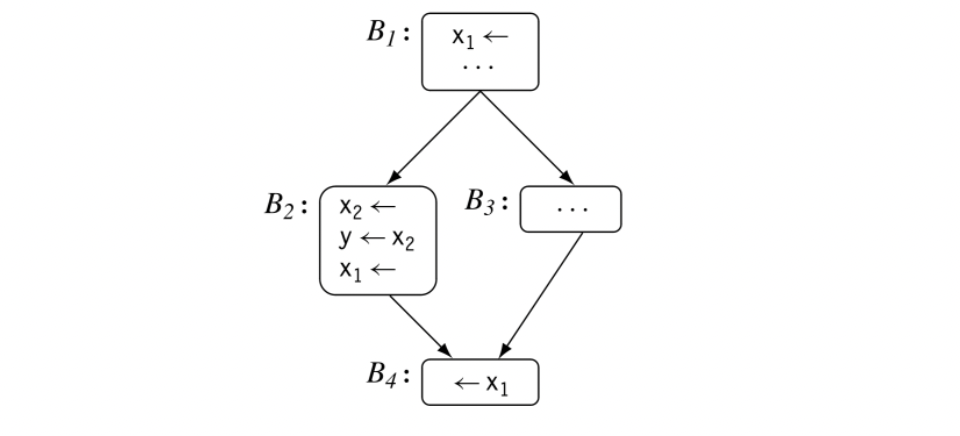Two LRs that use physically distinct classes of registers cannot interfere because they do not compete for the same resource. Thus, for example, a floating-point LR cannot interfere with an integer LR on a processor that uses distinct registers for these two kinds of values.

In the example CFG in the margin, the two LRs for x do not interfere; x2 is only live inside $β_{2}$ , in a stretch of code where x1 is dead. Thus, the allocation decisions for x1 and x2 are independent. They could share a PR, but there is no inherent reason for the allocator to make that choice.

Interference graph a graph $G = (N, E)$ that has a node n for each LR and an edge $(L_{R}, L_{i})$ if and only if $L R_{i}$ and $L R_{j}$ interfere

Global allocators operate by finding interferences and using them to guide the allocation process. The allocator described in Section 13.4 builds a concrete representation of these conflicts, an interference graph, and constructs a coloring of the graph to map live ranges onto Prs. Many global allocators follow this paradigm; they vary in the graph's precision and the specific coloring algorithm used.

Finding Interferences

To discover interferences, the compiler first computes live information for the code. Then, it visits each operation in the code and adds interferences. If the operation defines $L R_{i}$ , the allocator adds an interference to every $L R_{j}$ that is live at that operation.

The one exception to this rule is a copy operation, $L R_{i} \leftarrow L R_{j}$ which sets the value of $L R_{i}$ to the value of $L R_{j}$ . Because the source and destination LRs have the same value, the copy operation does not create an interference between them. If $L R_{i}$ and $L R_{j}$ do not otherwise interfere, they could occupy the same PR.

Interference and Register Pressure

Register pressure a term often used to refer to the demand for registers

The interference graph provides a quick way to estimate the demand for registers, often called register pressure. For a node $L R_{i}$ in the graph, the degree of $L R_{i}$ , written $L R_{i}^{\circ}$ , is the number of neighbors that $L R_{i}$ has in the graph. If all of $L R_{i}$ 's neighbors are live at the same operation, then $L R_{i}^{\circ} + 1$ registers would be needed to keep all of these values in registers. If those values are not all live at the same operation, then the register pressure may be lower than the degree. Maximum degree across all the nodes in the interference graph provides a quick upper bound on the number of registers required to execute the program without any spilling.

Representing Physical Registers

Often, the allocator will include nodes in the interference graph to represent Prs. These nodes allow the compiler to specify both connections to PRs and interferences with Prs. For example, if the code passes $L R_{i}$ as the second parameter at a call site, the compiler could record that fact with a copy from $L R_{i}$ to the PR that will hold the second parameter.

Pseudointerference If the compiler adds an edge between $L R_{i}$ and $P R_{j}$ , it must recognize that the edge does not actually contribute to demand for registers.

Some compilers use Prs to control assignment of an LR. To force $L R_{i}$ into $P R_{j}$ , the compiler can add a pseudointerference from $L R_{i}$ to every PR except $P R_{j}$ . Similarly, to prevent $L R_{i}$ from using $P R_{j}$ , the compiler can add an interference between $L R_{i}$ and $P R_{j}$ . While this mechanism works, it can become cumbersome. The mechanism for handling overlapping register classes presented in Section 13.4.7 provides a more general and elegant way to control placement in a specific PR.

13.2.3 Spill Code

When the allocator decides that it cannot keep some LR in a register, it must spill that LR to memory before reallocating its PR to another value. It must also restore the spilled LR into a PR before any subsequent use. These added spills and restores increase execution time, so the allocator should insert as few of them as practical. The most direct measure of allocation quality is the time spent in spill code at runtime.

Allocators differ in the granularity with which they spill values. The global allocator described in Section 13.4 spills the entire live range. When it decides to spill LR, it inserts a spill after each definition in LR and a restore immediately before each use of LR. In effect, it breaks LR into a set of tiny Lrs, one at each definition and each use.

By contrast, the local allocator described in Section 13.3 spills a live range only between the point where its PR is reallocated and its next use. Because it operates in a single block, with straight-line control flow, it can easily implement this policy; the LR has a unique next use and the point of spill always precedes that use.

Between these two policies, "spill everywhere" and "spill once," lie many possible alternatives. Researchers have experimented with spilling partial live ranges. The problem of selecting an optimal granularity for spilling is, undoubtedly, as hard as finding an optimal allocation; the correct granularity likely differs between live ranges. Section 13.5 describes some of the schemes that compiler writers and researchers have tried.

Nonuniform Spill Costs

To further complicate spilling, the allocator should account for the fact that properties of an LR can change the cost to spill it and to restore it.

An LR might be clean due to a prior spill along the current path, or because its value also exists in memory.

Dirty ValueIn the general case, the LR contains a value that has been computed and has not yet been stored to memory; we say that the LR is dirty. A dirty LR requires a store at its spill points and a load at its restore points.

Clean Value If the LR's value already exists in memory, then a spill does not require a store; we say that the LR is clean. A clean LR costs nothing to spill; its restores cost the same as those of a dirty value.

Rematerializable Value Some Lrs contain values that cost less to recompute than to spill and restore. If the values used to compute the LR'svalue are available at each use of the LR, the allocator can simply recompute the LR's value on demand. A classic example is an LR defined by an immediate load. Such an LR costs nothing to spill; to restore it, the compiler inserts the recomputation. Typically, an immediate load is cheaper than a load from memory.

The allocator should, to the extent possible, account for the nonuniform nature of spill costs. Of course, doing so complicates the allocator. Furthermore, the NP-complete nature of allocation suggests that no simple heuristic will make the best choice in every situation.

Spill Locations

Spill location a memory address associated with an LR that holds its value when the LR has no PR

When the allocator spills a dirty value, it must place the value somewhere in memory. If the LR corresponds precisely to a variable kept in memory, the allocator could spill the value back to that location. Otherwise, it must reserve a location in memory to hold the value during the time when the value is live and not in a PR.

Note that any value in a spill location is unambiguous, an important point for postal- location scheduling.

Most allocators place spill locations at the end of the procedure's local data area. This strategy allows the spill and restore code to access the value at a fixed offset from the ARP, using an address-immediate memory operation if the ISA provides one. The allocator simply increases the size of the local data area, at compile time, so the allocation incurs no direct runtime cost.

Because an LR is only of interest during that portion of the code where it is live, the allocator has the opportunity to reduce the amount of spill memory that it uses. If LR and LR do not interfere, they can share the same spill location. Thus, the allocator can also use the interference graph to color spill locations and reduce memory use for spills.

13.2.4 Register Classes

Register class a distinct group of named registers that share common properties, such as length and supported operations

Many processors support multiple classes of registers. For example, most ISAs have a set of general purpose registers (GPRs) for use in integer operations and address manipulation, and another set of floating-point registers (FPRs). In the case of GPRs and FPRs, the two register classes are, almost always, implemented with physically and logically disjoint register sets.

Often, an ISA will overlay multiple register classes onto a single physical register set. As shown in Fig. 13.2(a), the ARM A-64 supports four sizes of floating-point values in one set of quad-precision (128 bit) FPRs. The 128-bit FPRs are named $Q 0, Q 1, ..., Q 31$ . Each Qi is overlaid with a 64-bit register $D i$ , a 32-bit register Si, and a 16-bit register Hi. The shorter registers occupy the low-order bits of the longer registers.

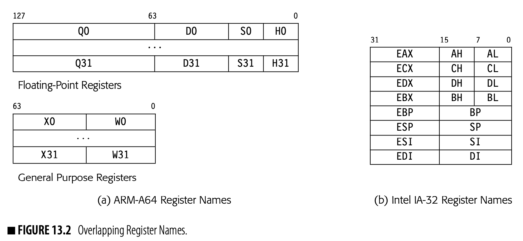
The ARM A-64 GPRs follow a similar scheme. The 64-bit GPRs have both 64-bit names Xi and 32-bit names Wi. Again, the 32-bit field occupies the low order bits of the 64-bit register.

The discussion focuses on a subset of the IA-32 register set. It ignores segment registers and most of the registers added in IA-64.

The Intel IA-32 has a small register set, part of which is depicted in Fig. 13.2(b). It provides eight 32-bit registers. The CISC instruction set uses distinct registers for specific purposes, leading to unique names for each register, as shown. For backward compatibility with earlier 16-bit processors, the PR set supports naming subfields of the 32-bit registers.

In four of the registers, the programmer can name the 32-bit register, its lower 16 bits, and two 8-bit fields. These registers are the accumulator (EAX), the count register (ECX), the data register (EDX), and the base register (EBX).
In the other four registers, the programmer can name both the 32-bit register and its lower 16 bits. These registers are the base of stack (EBP), the stack pointer (ESP), the string source index pointer (ESI), and the string destination index pointer (EDI).

The figure omits the instruction pointer (EIP and IP) and flag register (FFLAGS and FLAGS), which have both 32-bit and 16-names. The later IA-64 features a larger set of 32-bit GPRs, but preserves the IA-32 names and features in the low numbered registers. Many earlier ISAs used pairing schemes in the FPR set. The drawing in the margin shows how a four register set might work. It would consist of the four 32-bit PRs, F0, F1, F2, and F3. 64-bit values occupy a pair of adjacent registers. If a register pair can begin with any register, then four pairs are possible: D0, D1, D2, and D3.

Some ISAs restrict a register-pair to begin with an odd-numbered register--an aligned pair. With aligned pairs, only the registers shown as D0 and D2 would be available. With aligned pairs, use of D0 precludes the use of F0 and F1. With unaligned pairs, use of D0 still precludes the use of F0 and F1. It also precludes the use of D1 and D3.

In general, the register allocator should make effective use of all available registers. Thus, it must understand the processor's register classes and include mechanisms to use them in a fair and efficient manner. For physically disjoint classes, such as floating-point and general purpose register classes, the allocator can simply allocate them independently. If floating-point spills use GPRs for address calculations, the compiler should allocate the GPRs first.

The design of the register-set name space affects the difficulty of managing register classes in the allocator. For example, the ARM A-64 naming scheme allows the allocator to treat all of the fields in a single PR as a single resource; it can use one of X0 or W0. By contrast, the IA-32 allows concurrent use of both Ah and AL. Thus, the allocator needs more complex mechanisms to handle the IA-32 register set. Section 13.4.7 explores how to build such mechanisms into a global graph-coloring register allocator.

Section review

The register allocator must decide, at each point in the code, which values should be kept in registers. To do so, it computes a name space for the values in the code, often called live ranges. The allocator must discover which live ranges cannot share a register--that is, which live ranges interfere with each other. Finally, it must assign some live ranges to registers and relegate some to memory. It must insert appropriate loads and stores to move values between registers and memory to enforce its decisions.

Review questions

Consider a block of straight-line code where the largest register pressure at an operation in the block is $j$ . Assume that the allocator is allowed to use $k$ registers. If $j = k$ , can the allocator map the live ranges onto the PRs without spilling?
Consider a procedure represented as $n$ ILOC operations. Can you bound the number of nodes and edges in the interference graph?

13.3 Local Register Allocation

Recall that a basic block is a maximal length sequence of straight-line code.

The simplest formulation of the register allocation problem is local allocation: consider a single basic block and a single class of $k$ PRs. This problem captures many of the complexities of allocation and serves as a useful introduction to the concepts and terminology needed to discuss global allocation. To simplify the discussion, we will assume that one block constitutes the entire program.

The input code uses source registers, written in code as $s r_{i}$ . The output code uses physical registers, written in code as either $p r_{i}$ or simply $r_{i}$ . The physical registers correspond, in general, to named registers in the target ISA.

The input block contains a series of three-address operations, each of which has the form $op_{1} sr_{1}, sr_{2} \Rightarrow sr_{n}$ . From a high-level view, the local register allocator rewrites the block to replace each reference to a source register (SR) with a reference to a specific physical register (PR). The allocator must preserve the input block's original meaning while it fits the computation into the $k$ PRs provided by the target machine.

If, at any point in the block, the computation has more than $k$ live values--that is, values that may be used in the future-then some of those values will need to reside in memory for some portion of their lifetimes. ( $k$ registers can hold at most $k$ values.) Thus, the allocator must insert code into the block to move values between memory and registers as needed to ensure that all values are in PRs when needed and that no point in the code needs more than $k$ PRs.

This section presents a version of Best's algorithm, which dates back to the original Fortran compiler. It is one of the strongest known local allocation algorithms. It makes two passes over the code. The first pass derives detailed knowledge about the definitions and uses of values; essentially, it computes Live information within the block. The second pass then performs the actual allocation.

Spill When the allocator moves a live value from a PR to memory, it spills the value.

Restore When the allocator retrieves a previously spilled value from memory, it restores the value.

Best's algorithm has one guiding principle: when the allocator needs a PR and they are all occupied, it should spill the PR that contains the value whose next use is farthest in the future. The intuition is clear; the algorithm chooses the PR that will reduce demand for PRs over the longest interval. If all values have the same cost to spill and restore, this choice is optimal. In practice, that assumption is rarely true, but Best's algorithm still does quite well.

To explain the algorithm it helps to have a concrete data structure. Assume a three-address, ILOC-like code, represented as a list of operations. Each operation, such as $mult sr_{1}, sr_{2} \Rightarrow sr_{3}$ is represented with a structure:

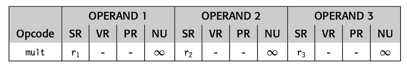
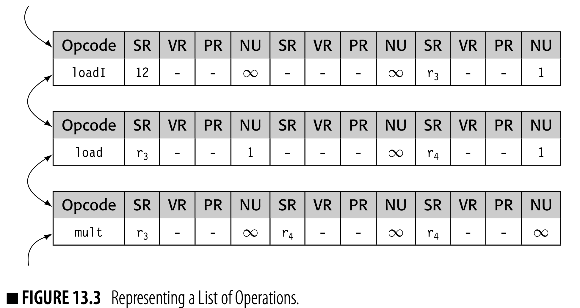
The operation has an opcode, two inputs (operands 1 and 2), and a result (operand 3). Each operand has a source-register name (SR), a virtual-register name (VR), a physical-register name (PR), and the index of its next use (NU).

Register allocation is, at its core, the process of constructing a new name space and modifying the code to use that space. Keeping the SR, VR, and PR names separate simplifies both writing and debugging the allocator.

A list of operations might be represented as a doubly linked list, as shown in Fig. 13.3. The local allocator will need to traverse the list in both directions. The list could be created in an array of structure elements, or with individually allocated or block-allocated structures.

Since the meaning is clear, we store a loadI’s constant in its first operand’s SR field.

The first operation, a load1, has an immediate value as its first argument, stored in the SR field. It has no second argument. The next operation, a load, also has just one argument. The final operation, a mult, has two arguments. Because the code fragment does not contain a next use for any of the registers mentioned in the mult operation, their NU fields are set to $\infty$ .

13.3.1 Renaming in the Local Allocator

To simplify the local allocator's implementation, the compiler can first rename SRs so that they correspond to live ranges. In a single block, an LR consists of a single definition and one or more uses. The span of the LR is the interval in the block between its definition and its last use.

The renaming algorithm finds the live range of each value in a block. It assigns each LR a new name, its VR name. Finally, it rewrites the code in terms of VRs. Renaming creates a one-to-one correspondence between LRs and VRs which, in turn, simplifies many of the data structures in the local allocator. The allocator then reasons about VRs, rather than arbitrary SR names.

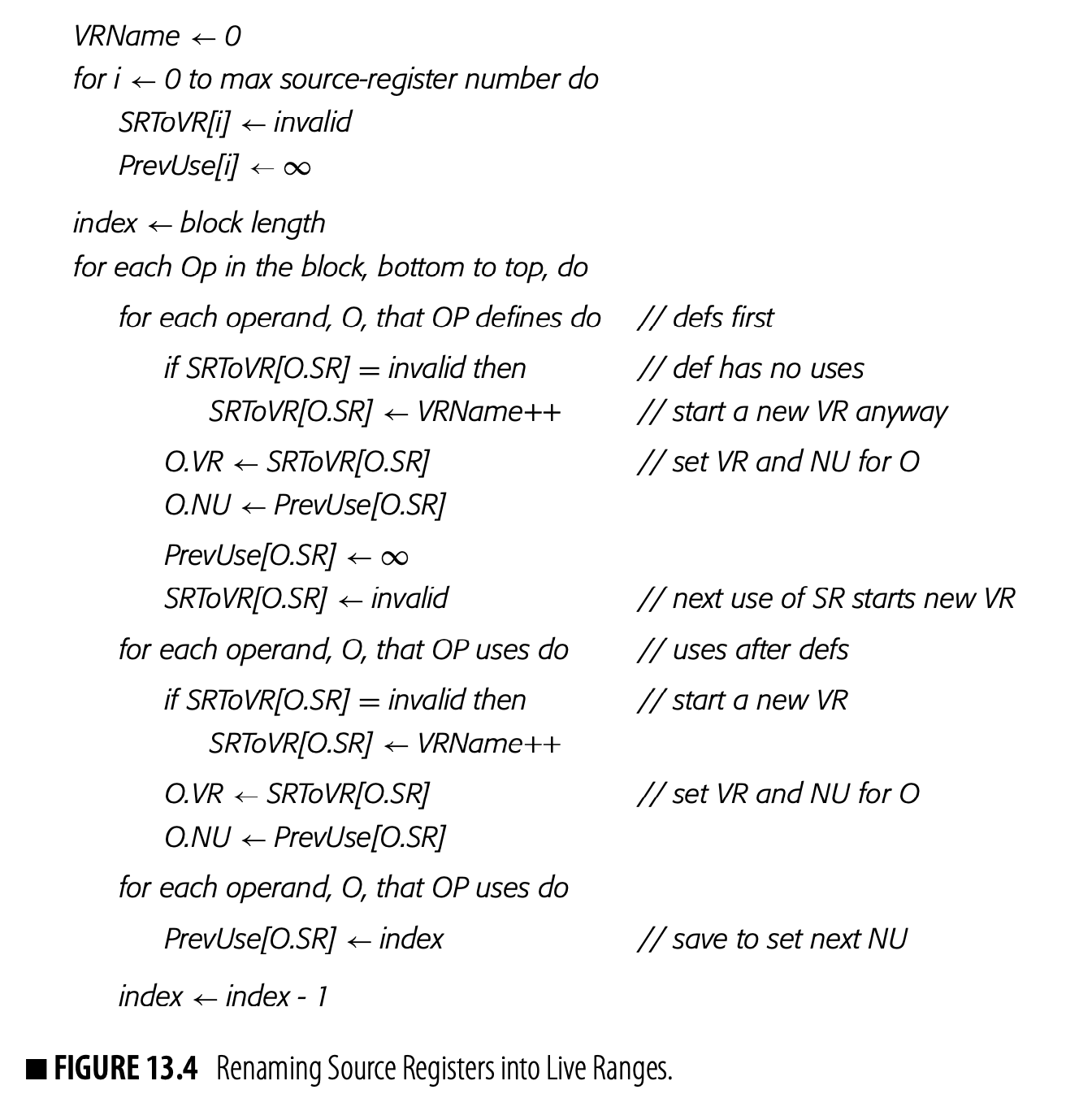
The compiler can discover live ranges and rename them into VRs in a single backward pass over the block. As it does so, it can also collect and record next use information for each definition and use in the block. The algorithm, shown in Fig. 13.4, assumes the representation described in the previous section.

The renaming algorithm builds two maps: SRToVR, which maps an SR name to a VR name, and PreUse, which maps an SR name into the ordinal number of its most recent use. The algorithm begins by initializing each SRToVR entry to invalid and each PrevUse entry to $\infty$ .

The algorithm walks the block from the last operation to the first operation. At each operation, it visits definitions first and then uses. At each operand, it updates the maps and defines the VR and NU fields.

If the SR for a definition has no VR, that value is never used. The algorithm still assigns a VR to the SR.

When the algorithm visits a use or def, it first checks whether or not the reference's SR, O.SR, already has a VR. If not, it assigns the next available VR name to the SR and records that fact in SRToVR[O.SR]. Next, it records the VR name and next use information in the operand's record. If the operand is a use, it sets PrevUse[O.SR] to the current operation's index. For a definition, it sets PrevUse[O.SR] back to \infty.

Note that all operands to a store are uses. The store defines a memory location, not a register.

The algorithm visits definitions before uses to ensure that the maps are updated correctly in cases where an SR name appears as both a definition and a use. For example, in add $r_{17}, r_{18} \Rightarrow r_{18}$ , the algorithm will rewrite the definition with $SRT o V R [r_{18}]$ ; update $SRT o V R [r_{18}]$ with a new VR name for the use; and then set $P re vU se [r_{18}]$ to $\infty$ .

After renaming, we use live range and virtual register interchangeably.

After renaming, each live range has a unique VR name. An SR name that is defined in multiple places is rewritten as multiple distinct VRs. In addition, each operand in the block has its NU field set to either the ordinal number of the next operation in the block that uses its value, or $\infty$ if it has no next use. The allocator uses this information when it chooses which VRs to spill.

Consider, again, the code from Fig. 13.1. $P an e l (a)$ shows the original code. $P an e l (b)$ shows that code after renaming. $P an e l (c)$ shows the span of each live range, as an interval graph. The allocator does not rename $r_{a r p}$ because it is a dedicated PR that holds the activation record pointer and, thus, not under the allocator's control.

MAXLIVE The maximum number of concurrently live VRs in a block

The maximum demand for registers, MAXLIVE, occurs at the start of the first mult operation, marked in panel (c) by the dashed gray line. Six VRs are live at that point. Both $VR_{7}$ and $VR_{8}$ are live at the start of the operation. The operation is the last use of $VR_{7}$ and $VR_{8}$ , as well as the definition of $VR_{5}$ .

13.3.2 Allocation and Assignment

The algorithm for the local allocator appears in Fig. 13.5. It performs allocation and assignment in a single forward pass over the block. It starts with an assumption that no values are in PRs. It iterates through the operations, in order, and incrementally allocates a PR to each VR. At each operation, the allocator performs three steps.

To ensure that a use has a PR, the allocator first looks for a PR in the VR-ToPR map. If the entry for VR is invalid, the algorithm calls GetAPR to find a PR. The allocator uses a simple marking scheme to avoid allocating the same PR to conflicting uses in a single operation.

If a single instruction contains multiple operations, the allocator should process all of the uses before any of the definitions.

In the second step, the allocator determines if any of the uses are the last use of the VR. If so, it can free the PR, which makes the PR available for reassignment, either to a result of the current operation or to some VR in a future operation.
In the third step, the allocator ensures that each VR defined by the operation has a PR allocated to hold its value. Again, the allocator uses GetAPR to find a suitable register.

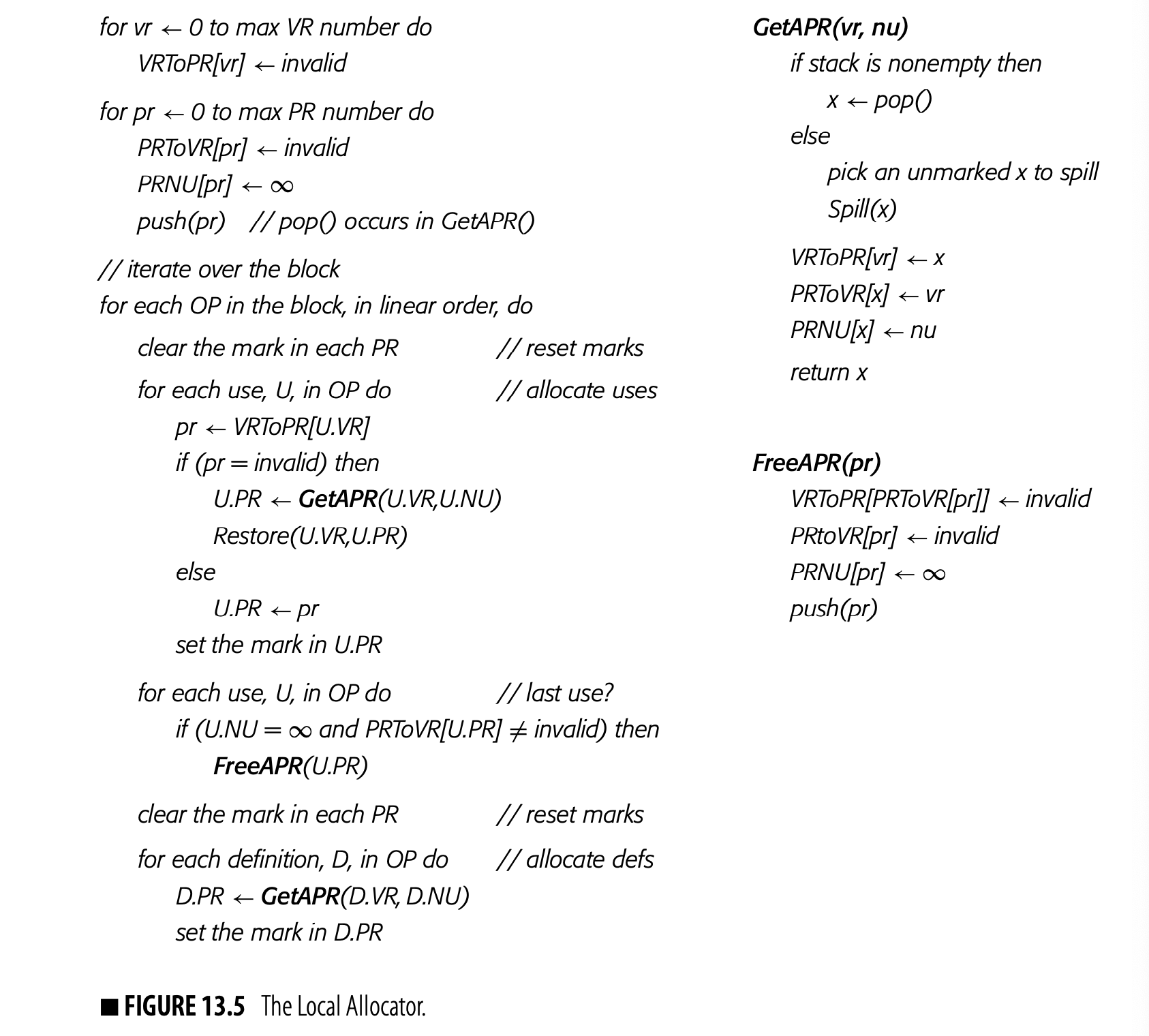
Each of these steps is straightforward, except for picking the value to spill. Most of the complexity of local allocation falls in that task.

The Workings of GetAPR

As it processes an operation, the allocator will need to find a PR for any VR $ν$ that does not currently have one. This act is the essential act of register allocation. Two situations arise:

Some PR $p$ is free: The allocator can assign $p$ to $ν$ . The algorithm maintains a stack of free Prs for efficiency.
No PR is free: The allocator must choose a VR to evict from its PR $p$ , save the value in $p$ to its spill location, and assign $p$ to hold $ν$ .

If the reference to $ν$ is a use, the allocator must then restore $ν$ 's value from its memory location to $p$ .

SPILL AND RESTORE CODE

At the point where the allocator inserts spill code, all of the physical registers (PRs) are in use. The compiler writer must ensure that the allocator can still spill a value.

Two scenarios are possible. Most likely, the target machine's ISA supports an address mode that allows the spill without need for an additional PR. For example, if the ARP has a dedicated register, say $r_{arp}$ , and the ISA includes an address-immediate store operation, like ILOC's storeAI, then spill locations in the local data area can be reached without an additional PR.

On a target machine that only supports a simple load and store, or an implementation where spill locations cannot reside in the activation record, the compiler would need to reserve a PR for the address computation, reducing the pool of available PRs. Of course, the reserved register is only needed if $M A X L I V E > k$ . (If $M A X L I V E \leq k$ , then no spills are needed and neither is the reserved register.)

Best's heuristic states that the allocator should spill the PR whose current VR has the farthest next use. The algorithm maintains PRNU to facilitate this decision. It simply chooses the PR with the largest PRNU. If the allocator finds two PRs with the same PRNU, it must choose one.

The implementation of PRNU is a tradeoff between the efficiency of updates and the efficiency of searches. The algorithm updates PRNU at each register reference. It searches PRNU at each spill. As shown, PRNU is a simple array; if updates are much more frequent than spills, that makes sense. If spills are frequent enough, a priority queue for PRNU may improve allocation time.

Tracking Physical and Virtual Registers

To track the relationship between VRs and Prs, the allocator maintains two maps. VRToPR contains, for each VR, either the name of the PR to which it is currently assigned, or the value invalid. PRToVR contains, for each PR, either the name of the VR to which it is currently assigned, or the value invalid.

As it proceeds through the block, the allocator updates these two maps so that the following invariant always holds: The code in GetAPR and FreeAPR maintains these maps to ensure that the invariant holds true. In addition, these two routines maintain PRNU, which maps a PR into the ordinal number of the operation where it is next used-a proxy for distance to that next use.

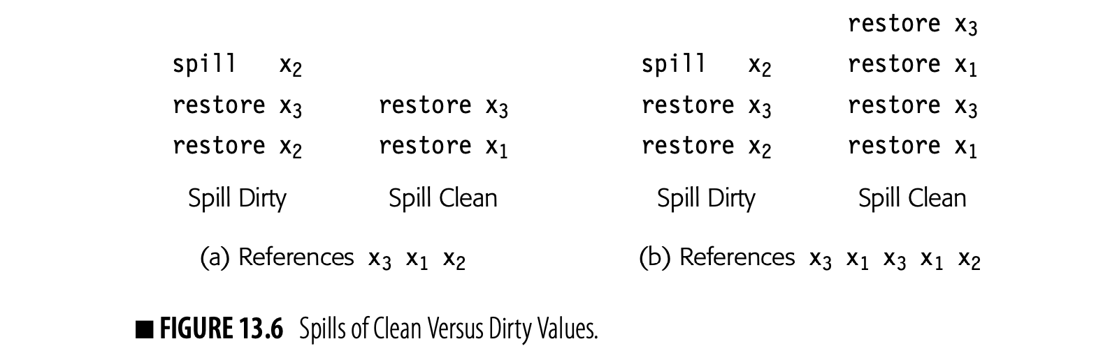
Spills and Restores

Conceptually, the implementation of Spill and Restore from Fig. 13.5 can be quite simple.

Spill locations typically are placed at the end of the local data area in the activation record.

To spill a PR p, the allocator can use PRToVR to find the VR $v$ that currently lives in p. If v does not yet have a spill location, the allocator assigns it one. Next, it emits an operation to store $p$ into the spill location. Finally, it updates the maps: VRTOPR, PRTOVR, and PRNU.
To restore a VR v into a PR p, the allocator simply generates a load from v 's spill location into p. As the final step, it updates the maps: VRToPR, PRTOVR, and PRNU.

If all spills have the same cost and all restores have the same cost, then Best's algorithm generates an optimal allocation for a block.

Complications from Spill Costs

In real programs, spill and restore costs are not uniform. Real code contains both clean and dirty values; the cost to spill a dirty value is greater than the cost to spill a clean value. To see this, consider running the local allocator on a block that contains references to three names, x_{1}, x_{2}, and x_{3}, with just two PRs (k=2).

Assume that the register allocator is at a point where x_{1} and x_{2} are currently in registers and x_{1} is clean and x_{2} is dirty. Fig. 13.6 shows how different spill choices affect the code in two different scenarios.

Reference string A reference string is just a list of references to registers or addresses. In this context, each reference is a use, not a definition.

Panel (a) considers the case when the reference string for the rest of the block is $x_{3} x_{1} x_{2}$ . If the allocator consistently spills clean values before dirty values, it introduces less spill code for this reference string.

Panel (b) considers the case when the reference string for the rest of the block is $x_{3} x_{1} x_{3} x_{1} x_{2}$ . Here, if the allocator consistently spills clean values before dirty values, it introduces more spill code.

The presence of both clean and dirty values fundamentally changes the lo- cal allocation problem. Once the allocator faces two kinds of values with different spill costs, the problem becomes NP-hard. The introduction of re- materializable values, which makes restore costs nonuniform, makes the problem even more complex. Thus, a fast deterministic allocator cannot always make optimal spill decisions. However, these local allocators can produce good allocations by choosing among LRs with different spill costs with relatively simple heuristics.

Remember, however, that the problem is NP-hard. No efficient, deterministic algo- rithm will always produce optimal results.

In practice, the allocator may produce better allocations if it differentiates between dirty, clean, and rematerializable values (see Section 13.2.3). If two PRs have the same distance to their next uses and different spill costs, then the allocator should spill the lower-cost PR.

The issue becomes more complex, however, in choosing between PRs with different spill costs that have next-use distances that are close but not iden- tical. For example, given a dirty value with next use of n and a rematerial- izable value with next use of $n - 1$ , the latter value will sometimes be the better choice.

Section Review

The limited context in local register allocation simplifies the problem enough so that a fast, intuitive algorithm can produce high-quality allocations. The local allocator described in this section operates on a simple principle: when a PR is needed, spill the PR whose next use is farthest in the future.

In a block where all values had the same spill costs, the local allocator would achieve optimal results. When the allocator must contend with both dirty and clean values, the problem becomes combinatorially hard. A local allocator can produce good results, but it cannot guarantee optimal results.

Review Questions

Modify the renaming algorithm, shown in Fig. 13.4, so that is also computes maxlive, the maximum number of simultaneously live values at any instruction in the block.
Rematerializing a known constant is an easy decision, because the spill requires no code and the restore is a single load immediate operation. Under what conditions could the allocator profitably rematerialize an operation such as add $r_{a}, r_{b} \Rightarrow r_{x}$ ?

13.4 Global Allocation via Coloring

Most compilers use a global register allocator--one that considers the entire procedure as context. The global allocator must account for more complex control flow than does a local allocator. Live ranges have multiple definitions and uses; they form complex webs across the control-flow graph. Different blocks execute different numbers of times, which complicates spill cost estimation. While some of the intuitions from local allocation carry forward, the algorithms for global allocation are much more involved.

Spilling an LR breaks it into small pieces that can be kept in distinct PRs.

A global allocator faces another complication: it must coordinate register use across blocks. In the local algorithm, the mapping from an enregistered LR to a PR is, essentially, arbitrary. By contrast, a global allocator must either keep an LR in the same register across all of the blocks where it is live or insert code to move it between registers.

Most global allocation schemes build on a single paradigm. They represent conflicts between register uses with an interference graph and then color that graph to find an allocation. Within this model, the compiler writer faces a number of choices. Live ranges may be shorter or longer. The graph may be precise or approximate. When the allocator must spill, it can spill that lr everywhere or it can spill the lr only in regions of high register pressure.

These choices create a variety of different specific algorithms. This section focuses on one specific set of choices: maximal length live ranges, a precise interference graph, and a spill-everywhere discipline. These choices define the global coloring allocator. Section 13.5 explores variations and improvements to the global coloring allocator.

Fig. 13.7 shows the structure of the global coloring allocator.

Find Live Ranges The allocator finds live ranges and rewrites the code with a unique name for each lr. The new name space ensures that distinct values are not constrained simply because they shared the same name in the input code.

Build Graph The allocator builds the interference graph. It creates a node for each lr and adds edges from $L R_{i}$ to any $L R_{j}$ that is live at an operation that defines $L R_{i}$ , unless the operation is a copy. Building the graph tends to dominate the cost of allocation.

Coalesce Copies The allocator looks at each copy operation, $L R_{i} \Rightarrow L R_{j}$ . If $L R_{i}$ and $L R_{j}$ do not interfere, it combines the lRs, removes the copy, and updates the graph. Coalescing reduces the number of lRs and reduces the degree of other nodes in the graph.

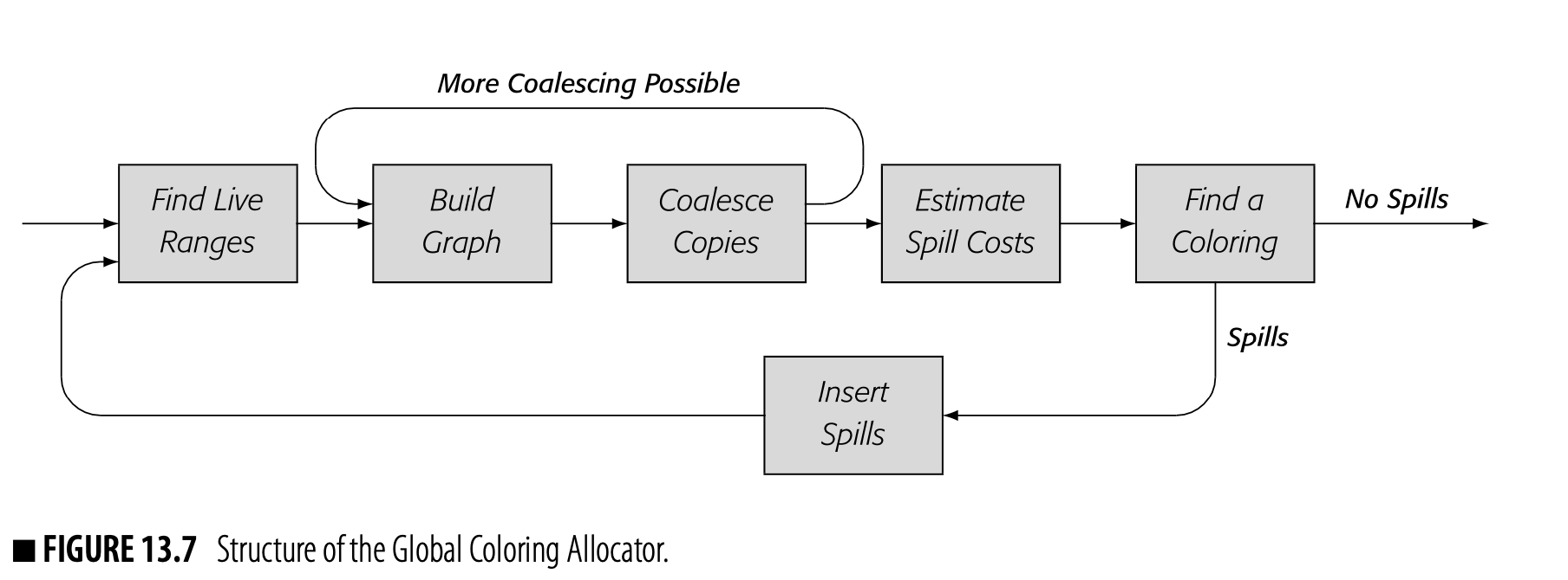
Unfortunately, the graph update is conservative rather than precise (see Section 13.4.3). Thus, if any LRs are combined, the allocator iterates the Build-Coolesce process until it cannot coalesce any more LRs--typically two to four iterations.

The spill cost computation has many corner cases (see Sections 13.2.3 and 13.4.4).

Estimate Spill Costs: The allocator computes, for each lr, an estimate of the runtime cost of spilling the entire lr. It adds the costs of the spills and restores, each multiplied by the estimated execution frequency of the block where the code would be inserted.

Find a Coloring: The allocator tries to construct a $k$ -coloring for the interference graph. It uses a two-phase process: graph simplification to construct an order for coloring, then graph reconstruction that assigns colors as it reinserts each node back into the graph.

If the allocator finds a $k$ -coloring, it rewrites the code and exits. If any nodes remain uncolored, the allocator invokes Insert Spills to spill the uncolored LRs. It then restarts the allocator on the modified code.

The second and subsequent attempts at coloring take less time than the first try because coalescing in the first pass has reduced the size of both the problem and the interference graph.

Insert Spills: For each uncolored lr, the allocator inserts a spill after each definition and a restore before each use. This converts the uncolored lr into a set of tiny LRs, one at each reference. This modified program is easier to color than the original code.

The following subsections describe these phases in more detail.

13.4.1 Find Global Live Ranges

GRAPH COLORING

Graph coloring is a common paradigm for global register allocation. For an arbitrary graph G, a coloring of G assigns a color to each node in G so that no pair of adjacent nodes has the same color. A coloring that uses k colors is termed a k-coloring, and the smallest such k for a given graph is called the graph’s minimum chromatic number. Consider the following graphs: The graph on the left is two-colorable. For example, we can assign blue to nodes 1 and 5 , and red to nodes 2,3 , and 4 . Adding the edge (2,3), as shown on the right, makes the graph three-colorable, but not two-colorable. (Assign blue to nodes 1 and 5 , red to nodes 2 and 4 , and yellow to node 3 .)

For a given graph, finding its minimum chromatic number is NP-complete. Similarly, determining if a graph is k-colorable, for fixed k, is NP-complete. Graph coloring allocators use approximate methods to find colorings that fit the available resources.

The maximum degree of any node in a graph gives an upper bound on the graph's chromatic number. A graph with maximum degree of $x$ can always be colored with $x + 1$ colors. The two graphs shown above demonstrate that degree is a loose upper bound. Both graphs have maximum degree of three. Both graphs have colorings with fewer than four colors. In each case, high-degree nodes have neighbors that can receive the same color.

As its first step, the global allocator constructs maximal-sized global live ranges (see Section 13.2.1). A global lr is a set of definitions and uses that contains all of the uses that a definition in the set can reach, along with all of the definitions that can reach those uses. Thus, the LR forms a complex web of definitions and uses that, ideally, should reside in a single PR.

The algorithm to construct live ranges is straightforward if the allocator can work from the SSA form of the code. Thus, the first step in finding live ranges is to convert the input code to SSA form, if necessary. The allocator can then build maximal-sized live ranges with a simple approach: at each $ϕ$ -function, combine all of the names, both definition and uses, into a single LR. If the allocator applies this rule at each $ϕ$ -function, it creates the set of maximal global LRs.

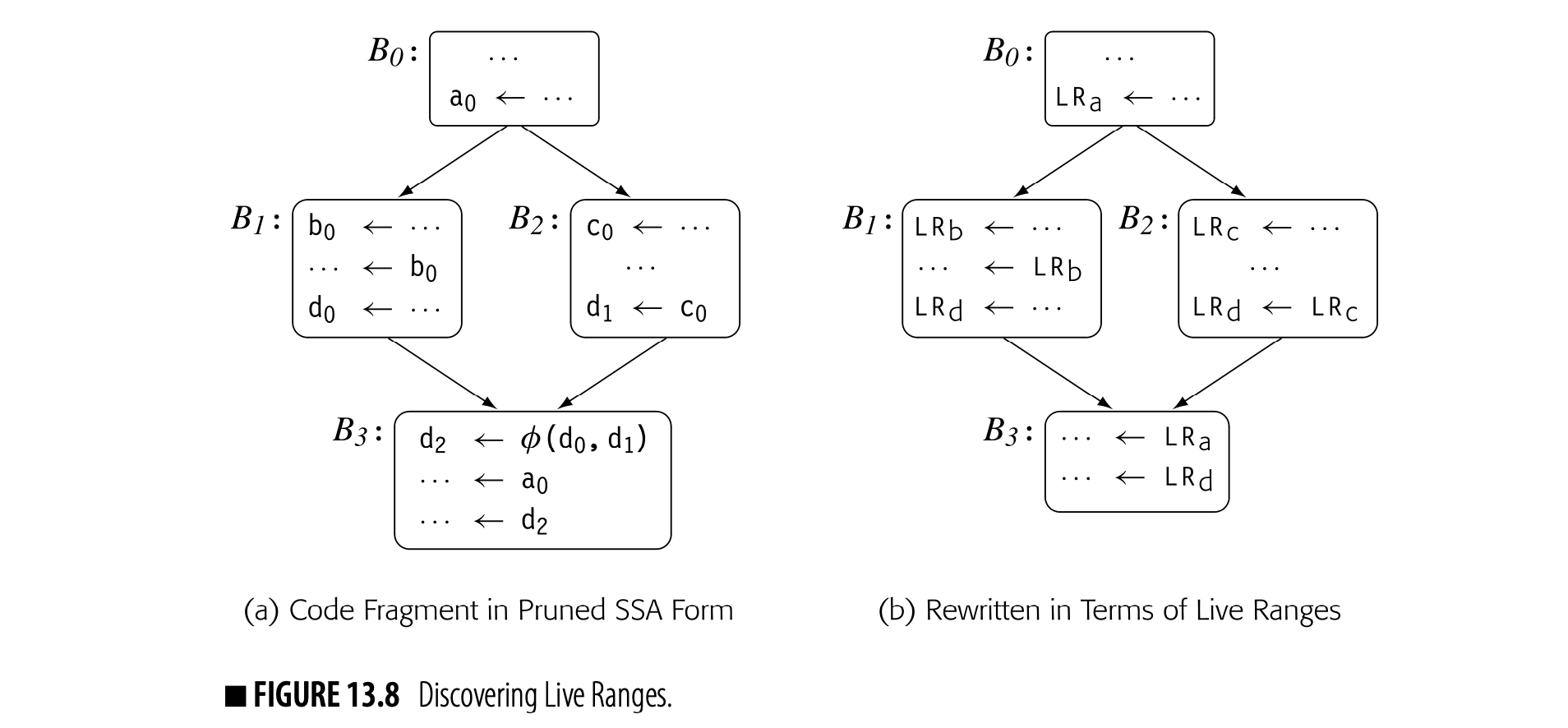
To make this process efficient, the compiler can use the disjoint-set union-find algorithm. To start, it assigns a unique set name to each SSA name. Next, it visits each $ϕ$ -function in the code and unions together the sets associated with each $ϕ$ -function parameter and the set for the $ϕ$ -function result. After all of the $ϕ$ -functions have been processed, each remaining unique set becomes an LR. The allocator can either rewrite the code to use LR names or it can create and maintain a mapping between SSA names and LR names. In practice, the former approach seems simpler.

Since the process of finding LRs does not move any definitions or uses, translation out of SSA form is trivial. The LR name space captures the effects that would require new copies during out-of-SSA translation. Thus, the compiler can simply drop the $ϕ$ -functions and SSA-names during renaming.

Fig. 13.8(a) shows a code fragment in semiprunned SSA form that involves source-code variables, a, b, c, and d. To find the live ranges, the allocator assigns each SSA name a set that contains its name. It unions together the sets associated with names used in the $ϕ$ -function, ${d_{0}} \cup {d_{1}} \cup {d_{2}}$ . This gives a final set of four LRs: $LR_{a} = {a_{0}}$ , $LR_{b} = {b_{0}}$ , $LR_{c} = {c_{0}}$ , and $LR_{d} = {d_{0}, d_{1}, d_{2}}$ . Fig. 13.8(b) shows the code rewritten to use the LRs.

13.4.2 Build an Interference Graph

To model interferences, the global allocator builds an interference graph, $I = (N, E)$ . Nodes in $N$ represent individual live ranges and edges in $E$ represent interferences between live ranges. Thus, an undirected edge $(n_{i}, n_{j}) \in E$ exists if and only if the corresponding live ranges $LR_{i}$ and $LR_{j}$ interfere. The interference graph for the code in Fig. 13.8(b) appears in the margin.

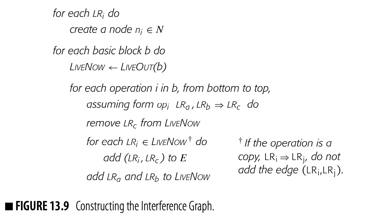
$L R_{a}$ interferes with each of $L R_{b}$ , $L R_{c}$ , and $L R_{d}$ . None of $L R_{b}$ , $L R_{c}$ , or $L R_{d}$ interfere with each other; they could share a single $PR$ .

If the compiler can color $I$ with $k$ or fewer colors, then it can map the colors directly onto $PR$ s to produce a legal allocation. In the example, $L R_{a}$ interferes with each of $L R_{b}$ , $L R_{c}$ , and $L R_{d}$ . In a coloring, $L R_{a}$ must receive its own color and, in an allocation, it cannot share a $PR$ with $L R_{b}$ , $L R_{c}$ , or $L R_{d}$ . The other live ranges do not interfere with each other. Thus, $L R_{b}$ , $L R_{c}$ , and $L R_{d}$ could share a single $color$ and, in the code, a single $PR$ . This interference graph is two-colorable, and the code can be rewritten to use just two registers. Now, consider what would happen if another phase of the compiler reordered the last two definitions in $B_{I}$ , as shown in the margin. This change makes $L R_{b}$ live at the definition of $L R_{d}$ . It adds an edge ( $L R_{b}$ , $L R_{d}$ ) to the interference graph, which makes the graph three-colorable rather than two-colorable. (The graph is small enough to prove this by enumeration.) With this new graph, the allocator has two options: to use three registers, or, if only two registers are available, to spill one of $L R_{b}$ or $L R_{a}$ before the definition of $L R_{d}$ in $B_{I}$ . Alternatively, the allocator could reorder the two operations and eliminate the interference between $L R_{b}$ and $L R_{d}$ . Typically, register allocators do not reorder operations. Instead, allocators assume a fixed order of operations and leave ordering questions to the instruction scheduler (see Chapter 12).

Section 11.3.2 also uses LIVENOW.

Given the code, renamed into $LR$ s, and $LiveOut$ sets for each block in the renamed code, the allocator can build the interference graph in one pass over each block, as shown in Fig. 13.9. The algorithm walks the block, from bottom to top. At each operation, it computes $LiveNow$ , the set of values that are live at the current operation. At the bottom of the block, $LiveOut$ and $LiveNow$ must be identical. As the algorithm walks backward through the block, it adds the appropriate interference edges to the graph and updates the LiveNow set to reflect each operation's impact.

The algorithm implements the definition of interference given earlier: $L R_{i}$ and $L R_{j}$ interfere only if $L R_{i}$ is live at a definition of $L R_{j}$ , or vice versa. The allocator adds, at each operation, an interference between the defined $L R$ and each $L R$ that is live after the operation.

Copy operations require special treatment. A copy $L R_{i} \Rightarrow L R_{j}$ does not create an interference between $L R_{i}$ and $L R_{j}$ because the two live ranges have the same value after the copy executes and, thus, could occupy the same register. If subsequent context creates an interference between these live ranges, that operation will create the edge. Treating copies in this way creates an interference graph that precisely captures when $L R_{i}$ and $L R_{j}$ can occupy the same register. As the allocator encounters copies, it should create a list of all the copy operations for later use in coalescing.

Insertion into the lists should check the bit-matrix to avoid duplication.

To improve the allocator's efficiency, it should build both a lower-triangular bit matrix and a set of adjacency lists to represent $E$ . The bit matrix allows a constant-time test for interference, while the adjacency lists allow efficient iteration over a node's neighbors. The two-representation strategy uses more space than a single representation would, but pays off in reduced allocation time. As suggested in Section 13.2.4, the allocator can build separate graphs for disjoint register classes, which reduces the maximum graph size.

13.4.3 Coalesce Copy Operations

The allocator can use the interference graph to implement a strong form of copy coalescing. If the code contains a copy operation, $L R_{i} \Rightarrow L R_{j}$ , and the allocator can determine that $L R_{i}$ and $L R_{j}$ do not interfere at some other operation, then the allocator can combine the $L R_{s}$ and remove the copy operation. We say that the copy has been "coalesced."

In his thesis, Briggs shows examples where coalescing eliminates up to one-third of the initial live ranges.

Coalescing a copy has several beneficial effects. It eliminates the actual copy operation, which makes the code smaller and, potentially, faster. It reduces the degree of any $L R$ that previously interfered with both $L R_{i}$ and $L R_{j}$ . It removes a node from the graph. Each of these effects makes the coloring pass faster and more effective.

Fig. 13.10 shows a simple, single-block example. The original code appears in panel (a). Intervals to the right indicate the extents of the live ranges that are involved in the copy operation. Even though $L R_{a}$ overlaps both $L R_{b}$ and $L R_{c}$ , it interferes with neither of them because the overlaps involve copy operations. Since $L R_{b}$ is live at the definition of $L R_{c}$ , $L R_{b}$ and $L R_{c}$ interfere. Both copy operations are candidates for coalescing.

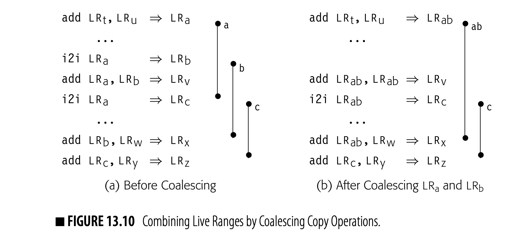
Fig. 13.10(b) shows the result of coalescing LR $_{a}$ and LR $_{b}$ to produce LR $_{ab}$ . LR $_{ab}$ and LR $_{c}$ still do not interfere, because LR $_{c}$ is created by the copy operation from LR $_{ab}$ . Combining LR $_{a}$ and LR $_{b}$ reduces LR $_{v}^{\circ}$ by one. Before coalescing, both LR $_{a}$ and LR $_{b}$ interfered with LR $_{v}$ . After coalescing, those values occupy a single LR rather than two LRs. In general, coalescing two live ranges either decreases the degrees of their neighbors or leaves them unchanged; it cannot increase their degrees.

The membership test should use the bit- matrix for efficiency.

To perform coalescing, the allocator walks the list of copies from Build Graph and inspects each operation, LR $_{i} \Rightarrow$ LR $_{j}$ . If $(LR_{i}, LR_{j}) \in / E$ , then LR $_{i}$ and LR $_{j}$ do not interfere and the allocator combines them, eliminates the copy, and updates $I$ to reflect the new, combined LR $_{ij}$ . The allocator can conservatively update $I$ by moving each edge from LR $_{i}$ and LR $_{j}$ to LR $_{ij}$ , eliminating duplicates. This update is not precise, but it lets the allocator continue coalescing.

In practice, allocators coalesce every live range that they can, given the interferences in $I$ . Then, they rewrite the code to reflect the revised LRs and eliminate the coalesced copies. Next, they rebuild $I$ and try again to coalesce copies. This process typically halts after a couple of rounds of coalescing.

The example illustrates the imprecise nature of this conservative update to the graph. The update moves the edge $(LR_{b}, LR_{c})$ from LR $_{b}$ to LR $_{ab}$ , when, in fact, LR $_{ab}$ and LR $_{c}$ do not interfere. Rebuilding the graph from the transformed code yields the precise interference graph, without $(LR_{ab}, LR_{c})$ . At that point, the allocator can coalesce LR $_{ab}$ and LR $_{c}$ .

If the allocator can coalesce LR $_{i}$ with either LR $_{j}$ or LR $_{k}$ , choosing to form LR $_{ij}$ may prevent a subsequent coalesce with LR $_{k}$ , or vice versa. Thus, the order of coalescing matters. In principle, the compiler should coalesce the most frequently executed copies first. Thus, the allocator might coalesce copies in order by the estimated execution frequency of the block that contains the copy. To implement this, the allocator can consider the basic blocks in order from most deeply nested to least deeply nested.

This strategy applies a lesson from semipruned SSA form: only include the names that matter.

In practice, the cost of building the interference graph for the first round of coalescing dominates the overall cost of the graph-coloring allocator. Subsequent passes through the build-coalesce loop process a smaller graph and, therefore, run more quickly. To reduce the cost of coalescing, the compiler can build a subset of the interference graph--one that only includes live ranges involved in a copy operation.

13.4.4 Estimate Global Spill Costs

When a register allocator discovers that it cannot keep all of the live ranges in registers, it must select an lr to spill. Typically, the allocator uses some carefully designed metric to rank the choices and picks the lr that its metric suggests is the best spill candidate. The local allocator used the distance to the lr's next use, which works well in a single-block context. In the global allocator, the metric incorporates an estimate of the runtime costs that will be incurred by spilling and restoring a particular lr.

To compute the estimated spill costs for an lr, the allocator must examine each definition and use in the lr. At each definition, it estimates the cost of a spill after the definition and multiplies that number by the estimated execution frequency of the block that contains the definition. At each use, it estimates the cost of a restore before the use and multiplies that number by the estimated execution frequency of the block that contains the use. It sums together the estimated costs for each definition and use in the lr to produce a single number. This number becomes the spill cost for the lr.

Of course, the actual computation is more complex than the preceding explanation suggests. At a given definition or use of an lr, the value might be any of dirty, clean, or rematerializable (see Section 13.2.3). Individual definitions and uses within an lr can have different classifications, so the allocator must perform enough analysis to classify each reference in the lr. That classification determines the cost to spill or restore that reference.

The precise execution count of a block is difficult to determine. Fortunately, relative execution frequencies are sufficient to guide spill decisions; the allocator needs to know that one reference is likely to execute much more often than another. Thus, the allocator derives, for each block, a number that indicates its relative execution frequency. Those frequencies apply uniformly to each reference in the block.

The allocator could compute spill costs on demand--when it needs to make a spill decision. If it finds a $k$ -coloring without any spills, an on-demandcost computation would reduce overall allocation time. If the allocator must spill frequently, a batch cost computation would, most likely, be faster than an on-demand computation.

Fig. 13.7 suggests that the allocator should perform the cost computation before it tries to color the graph. The allocator can defer the computation until the first time that it needs to spill. If the allocator does not need to spill, it avoids the overhead of computing spill costs; if it does spill, it computes spill costs for a smaller set of LRs.

Accounting for Execution Frequencies

Using the 1 $0^{d}$ estimator can introduce a problem with integer overflow in the spill cost computation. Many compiler writers have discovered this issue experimentally. Deeply nested loops may need floating-point spill costs.

To compute spill costs, the allocator needs an estimate of the execution frequency for each basic block. The compiler can derive these estimates from profile data or from heuristics. Many compilers assume that each loop executes 10 times, which creates a weight of $1 0^{d}$ for a block nested inside $d$ loops. This assumption assigns a weight of 10 to a block inside one loop, 100 to a block inside two nested loops, and so on. An unpredictable if-then-else would decrease the estimated frequency by half. In practice, these estimates create a large enough bias to encourage spilling LRs in outer loops rather than those in inner loops.

Negative Spill Costs

A live range that contains a load, a store, and no other uses should receive a negative spill cost if the load and store refer to the same address. (Optimization can create such live ranges; for example, if the use were optimized away and the store resulted from a procedure call rather than the definition of a new value.) Sometimes, spilling a live range may eliminate copy operations with a higher cost than the spill operations; such a live range also has a negative cost. Any live range with a negative spill cost should be spilled, since doing so decreases demand for registers and removes operations from the code.

Infinite Spill Costs

Some live ranges are so short that spilling them does not help. Consider the short LR shown in the left margin. If the allocator tries to spill LR, it will insert a store after the definition and a load before the use, creating two new LRs. Neither of these new LRs uses fewer registers than the original LR, so the spill produces no benefit. The allocator should assign the original LR a spill cost of infinity, ensuring that the allocator does not try to spill it. In general, an LR should have infinite spill cost if no other LR ends between its definitions and its uses. This condition stipulates that availability of registers does not change between the definitions and uses.

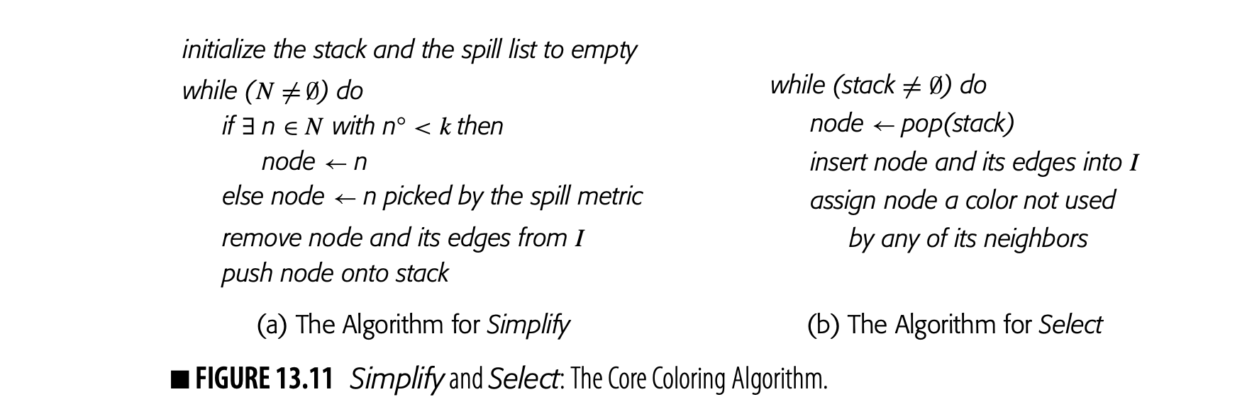
Infinite-cost live ranges present a code-shape challenge to the compiler. If the code contains more than $k - 1$ nested infinite-cost LRs, and no LR ends in this region, then the infinite-cost LRs form an uncolorable clique in the interference graph. While such a situation is unusual, we have seen it arise in practice. The register allocator cannot fix this problem; the compiler writer must simply ensure that the allocator does not receive such code.

13.4.5 Color the Graph

The global allocator colors the graph in a two-step process. The first step, called Simplify, computes an order in which to attempt the coloring. The second step, called Select, considers each node, in order, and tries to assign it a color from its set of $k$ colors.

To color the graph, the allocator relies on a simple observation:

If a node has fewer than $k$ neighbors, then it must receive a color, independent of the colors assigned to its neighbors.

Thus, any node $n$ with degree less than $k$ , denoted $n^{\circ} < k$ , is trivial to color. The allocator first tries to color those nodes that are hard to color; it defers trivially colored nodes until after the difficult nodes have been colored.

Simplify

To compute an order for coloring, the allocator finds trivially colored nodes and removes them from the graph. It records the order of removal by pushing the nodes onto a stack as they are removed. The act of removing a node and its edges from the graph lowers the degree of all its neighbors. Fig. 13.11(a) shows the algorithm.

As nodes are removed from the graph, the allocator must preserve both the node and its edges for subsequent reinsertion in Select. The allocator can either build a structure to record them, or it can add a mark to each edge and each node indicating whether or not it is active.

Spill metric a heuristic used to select an LR to spill

Sirplify uses two distinct mechanisms to select the node to remove next. If there exists a node $n$ with $n^{\circ} < k$ , the allocator chooses that node. Because these nodes are trivially colored, the order in which they are removed does not matter. If all remaining nodes are constrained, with degree $\geq k$ , then the allocator picks a node to remove based on its spill metric. Any node $n$ removed by this process has $n^{\circ} \geq k$ ; thus, it may not receive a color during the assignment phase. The loop halts when the graph is empty. At that point, the stack contains all the nodes in order of removal.

Select

To color the graph, the allocator rebuilds the interference graph in the reverse of the removal order. It repeatedly pops a node $n$ from the stack, inserts $n$ and its edges back into $I$ , and picks a color for $n$ that is distinct from $n$ 's neighbors. Fig. 13.11(b) shows the algorithm.

In our experience, the order in which the allocator considers colors has little practical impact.

To select a color for node $n$ , the allocator tallies the colors of $n$ 's neighbors in the current graph and assigns $n$ an unused color. It can search the set of colors in a consistent order, or it can assign colors in a round-robin fashion. If no color remains for $n$ , it is left uncolored.

When the stack is empty, $I$ has been rebuilt. If every node has a color, the allocator rewrites the code, replacing LR names with pr names, and returns. If any nodes remain uncolored, the allocator spills the corresponding LRs. The allocator passes a list of the uncolored LRs to insert Spills, which adds the spills and restores to the code. Insert Spills then restarts the allocator on the revised code. The process repeats until every node in $I$ receives a color. Typically, the allocator finds a coloring and halts in a couple of trips around the large loop in Fig. 13.7.

Why Does This Work?

The global allocator inserts each node back into the graph from which it was removed. If the reduction algorithm removes the node for $LR_{n}$ from $I$ because $n^{\circ} < k$ , then it reinserts $LR_{n}$ into a graph in which $n^{\circ} < k$ and node $n$ is trivially colored.

The only way that a node $n$ can fail to receive a color is if $n$ was removed from $I$ using the spill metric. Select reinserts such a node into a graph in which $n^{\circ} \geq k$ . Notice, however, that this condition is a statement about degree in the graph, rather than a statement about the availability of colors.

If node $n$ 's neighbors use all $k$ colors, then the allocator finds no color for $n$ . If, instead, they use fewer than $k$ colors, then the allocator finds a color for $n$ . In practice, a node $n$ often has multiple neighbors that use the same color. Thus, Select often finds colors for some of these constrained nodes.

Updating the Interference Graph Both coalescing and spilling change the set of nodes and edges in the interference graph. In each case, the graph must be updated before allocation can proceed.

The global coloring allocator uses a conservative update after each coalesce; that update also triggers another iteration around the Build-Coalesce loop in Fig. 13.7.It obtains precision in the graph by rebuilding it from scratch.

The allocator defers spill insertion until the end of the Simplify-Select process; it then inserts all of the spill code and triggers another iteration of the Build-Coalesce-Spill Costs-Color loop. Again, it obtains precision by rebuilding the graph.

If the allocator could update the graph precisely, it could eliminate both of the cycles shown in Fig. 13.7. Coalescing could complete in a single pass. It could insert spill code incrementally when it discovered an uncolored node; the updated graph would correctly reflect interferences for color selection.

Better incremental updates can reduce allocation time. A precise update would produce the same allocation as the original allocator, within variance caused by changes in the order of decisions. An imprecise but conservative update could produce faster allocations, albeit with some potential decrease in code quality from the imprecision in the graph. DasGupta

Simplify determines the order in which Select tries to color nodes. This order plays a critical role in determining which nodes receive colors. For a node $n$ removed from the graph because $n^{\circ} < k$ , the order is unimportant with respect to the nodes that remain in the graph. The order may be important with respect to nodes already on the stack; after all, $n$ may have been constrained until some of those earlier nodes were removed. For nodes removed from the graph using the spill metric, the order is crucial. The else clause in Fig. 13.11(a) executes only when every remaining node has degree $\geq k$ . Thus, the nodes that remain in the graph at that point are in more heavily connected subgraphs of $I$ .

The original global coloring allocator appeared in IBM’s PL.8 compiler.

The order of the constrained nodes is determined by the spill metric. The original coloring allocator picked a node that minimized the ratio of $cos t \div d e g ree$ , where $cos t$ is the estimated spill cost and $d e g ree$ is the node's degree in the current graph. This metric balances between spill cost and the number of nodes whose degree will decrease.

Other spill metrics have been tried. Several metrics are variations on $cos t \div d e g ree$ , including $cos t \div d e g re e^{2}$ , $cos t \div a re a$ and $cos t \div a re a^{2}$ , where the $a re a$ of an LR is defined as the sum of MAXLIVE taken over all theinstructions that lie within the LR. These metrics try to balance the cost of spilling a specific LR against the extent to which that spill makes it easier to color the rest of the graph. Straight cost has been tried; it focuses on runtime speed. In code-space sensitive applications, a metric of total spill operations can drive down the code-space growth from spilling.

In practice, no single heuristic dominates the others. Since coloring is fast relative to building $I$ , the allocator can color $I$ with several different spill metrics and keep the best result.

13.4.6 Insert Spill and Restore Code

The spill code created by a global register allocator is no more complex than the spill code inserted in the local allocator. Insert Spills receives a list of Lrs that did not receive a color. For each LR, it inserts the appropriate code after each definition and before each use.

The same complexities that arose in the local allocator apply in the global case. The allocator should recognize the distinction between dirty values, clean values, and rematerializable values. In practice, it becomes more complex to recognize whether a value is dirty, clean, or rematerializable in the global scope.

The global allocator applies a spill everywhere discipline. An uncolored live range is spilled at every definition point and restored at every use point. In practice, a spilled LR often has definitions and uses that occur in regions where Prs are available. Several authors have looked at techniques to loosen the spill everywhere discipline so as to keep spilled Lrs in Prs in regions of low register pressure (see the discussions in Section 13.5).

13.4.7 Handling Overlapping Register Classes

In practice, the register allocator must deal with the idiosyncratic properties of the target machine's register set and its calling convention. This reality constrains both allocation and assignment.

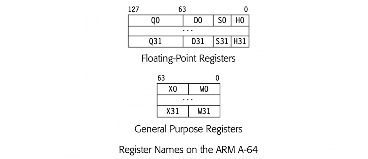
For example, on the ARM A-64, the four floating-point registers Q1, Q1, S1, and H1 all share space in a single PR, as shown in the margin. Thus, if the compiler allocates Q1 to hold LRi, Q1, S1, and H1 are unavailable while LRi is live. Similar restrictions arise with the overlapped general purpose registers, such as the pair X3 and W3.

To understand how overlapping register classes affect the structure of a register allocator, consider how the local allocator might be modified to handle the ARM A-64 general purpose registers.

The algorithm, as presented, uses one attribute to describe an LR, its virtual register number. With overlapping classes, such as Xi and Wi, each LR also needs an attribute to describe its class.

The stack of free registers should use names drawn from one of the two sets of names, Xi or Wi. The state, allocated or free, of a coresident pair such as X0 and WO is identical.
The mappings VRT0PR, PRT0VR, and PRNU can also remain single-valued. If $V R_{i}$ has an allocated register, VRT0PR will map the vr's num field to a register number and its class field will indicate whether to use the X name or the W name.

Because the local algorithm has a simple way of modeling the status of the prs, the extensions are straightforward. 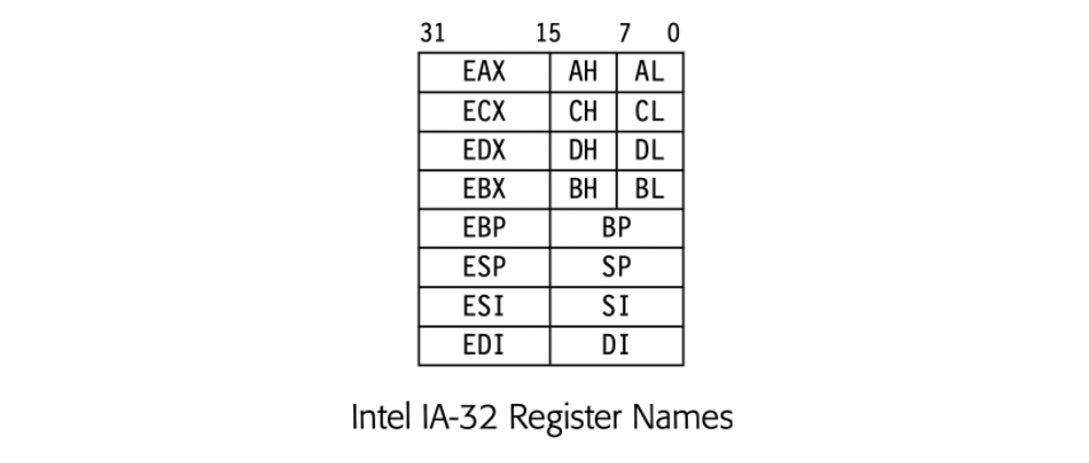To handle a more complex situation, such as the EAX register on the IA-32, the local allocator would need more extensive modifications. Use of EAX requires the entire register and precludes simultaneous use of AH or AL. Similarly, use of either AH or AL precludes simultaneous use of EAX. However, the allocator can use both AL and AH at the same time. Similar idiosyncratic rules apply to the other overlapping names, shown in the margin and in Fig. 13.2(b).

The global graph-coloring allocators have more complex models for interference and register availability than the local allocator. To adapt them for fair use of overlapping register classes requires a more involved approach.

Describing Register Classes

Before we can describe a systematic way to handle allocation and assignment for multiple register classes, we need a systematic way to describe those classes. The compiler can represent the members of each class with a set. From Fig. 13.2(a), the ARM A-64 has six classes:

Thus, $class (D3) = {00, 01, \dots, 031}$ , the set of 64-bit floating-point registers.

The simplest scheme to describe overlap between register classes is to introduce a function, $alias (r)$ . For a register name $r$ , $alias (r)$ maps $r$ to the set of register names that occupy physical space that intersects with $r$ 's space. In the ARM A-64, $alias (WI) = {X1}$ and $alias (S2) = {02, 02, 02}$ . Similarly, in IA-32, $alias (AH) = {EA}$ , $alias (AL) = {EA}$ , and $alias (EAX) = {AL, AH}$ . Because AL and AH occupy disjoint space, they are not aliases of each other.

The compiler can compute the information that it will need for allocation and assignment from the class and alias relationships.

Coloring with Overlapping Classes

The presence of overlapping register classes complicates each of coloring, assignment, and coalescing.

Coloring

The graph-coloring allocator approximates colorability by comparing a node's degree against the number of available colors. If $n^{\circ} < k$ , the number of available registers, then Simplify categorizes $n$ as trivially colored, removes $n$ from the graph, and pushes $n$ onto the ordering stack. If the graph contains no trivially colored node, Simplify chooses the next node for removal using its spill metric.

The presence of multiple register classes means that $k$ may vary across classes. For the node $n$ that represents $L R_{n}$ , $k = ∣ class (L R_{n}) ∣$ .

The presence of overlapping register classes further complicates the approximation of colorability. If the LR's class has no aliases, then simple arithmetic applies; a single neighbor reduces the supply of possible registers by one. If the LR's class has aliases--that is, register classes overlap--then it may be the case that a single neighbor can reduce the supply of possible registers by more than one.

In IA-32, EAX removes both AH and AL; it reduces the pool of 8-bit registers by two. The relationship is not symmetric; use of AL does not preclude use of AH. Unaligned floating-point register pairs create a more general version of this problem.
By contrast, the ARM A-64 ensures that each neighbor counts as one register. For example, W2 occupies the low-order 32 bits of an X2 register; no name exists for X2's high-order bits. Floating-point registers have the same property; only one name at each precision is associated with a given 128-bit register (Qi).

To extend Simplify to work fairly and correctly with overlapping register classes, we must replace $n^{\circ} < k$ with an estimator that conservatively and correctly estimates colorability in the more complex case of overlapping register classes. Rather than tallying $n$ 's neighbors, we must count those neighbors with which $n$ competes for registers.

Smith, Ramsey, and Holloway describe an efficient estimator that provides a fair and correct estimate of colorability. Their allocator precomputes supporting data from the class and alias relationships and then estimates $n$ 'scolorability based on $n$ 's class and the registers assigned to its relevant neighbors.

Assignment

Traditional discussions of graph-coloring allocators assume that the assignment of specific registers to specific live ranges does not have a significant impact on colorability. The literature ignores the difference between choosing colors "round-robin" and "first-in, first-out," except in unusual cases, such as biased coloring (see Section 13.5.1).

With overlapping register classes, some register choices can tie up more than one register. In IA-32, using EAX reduces the supply of eight bit registers by two, Ah and AL, rather than one. Again, unaligned floating-point register pairs create a more general version of the problem. Just as one register assignment can conflict with multiple others, so too can one assignment alter the available incremental choices.

Consider looking for a single eight bit register on IA-32. If the available options were AL and CL, but AH was occupied and CH was not, then choosing AL might introduce fewer constraints. Because EAX already conflicts with AH, the choice of AL does not reduce the set of available E registers. By contrast, choosing CL would make ECX unavailable. Overlapping register classes complicate assignment enough to suggest that the allocator should choose registers with a more complex mechanism than the first-in, first-out stack from Section 13.3.

Coalescing

The compiler should only coalesce two LRs, $LR_{i}$ and $LR_{j}$ , if the resulting live range has a feasible register class. If both are general purpose registers, for example, then the combination works. If $class (LR_{i})$ contains only $PR_{2}$ and $class (LR_{j})$ contains only $PR_{4}$ , then the allocator must recognize that the combined $LR_{ij}$ would be overconstrained (see the further discussion in Section 13.5.1).

Coloring with Disjoint Classes

If the architecture contains sets of classes that are disjoint, the compiler can allocate them separately. For example, most processors provide separate resources for general purpose registers and floating-point registers. Thus, allocation of $LR_{i}$ to a floating-point register has no direct impact on allocation in the general purpose register set. Because spills of floating-point values may create values that need general purpose registers, the floating-point allocation should precede the general purpose allocation.

If the allocator builds separate graphs for disjoint subclasses, it can reduce the number of nodes in the interference graph, which can yield significant compile-time savings, particularly during Build Graph.

Forcing Specific Register Placement

The allocator must handle operations that require placement of live ranges in specific PRs. These constraints may be either restrictions (LR $_{i}$ must be in PR $_{j}$ ) or exclusions (LR $_{i}$ cannot be in PR $_{k}$ ).

These constraints arise from several sources. The linkage convention dictates the placement of values that are passed in registers; these constraints include the ARP, some or all of the actual parameters, and the return value. Some hardware operations may require their operands in particular registers; for example, the 16-bit signed multiply on the IA-32 always reads an argument from AX and writes to both AX and DX.

The register class mechanism creates a simple way to handle such restrictions. The compiler writer creates a small register class for this purpose and attaches that class to the appropriate LRs. The coloring mechanism handles the rest of the details.

To handle exclusions, the compiler writer can build an exclusion set, again, a list of PRs, and attach it to specific LRs. The coloring mechanism can test prospective choices against the exclusion set. For example, between the code that saves the caller-saves registers and the code that restores them, the allocator should not use the caller-saves registers to hold anything other than a temporary value. A simple exclusion set will ensure this safe behavior.

Section Review

Global register allocators operate over entire procedures. The presence of control flow makes global allocation more complex than local allocation. Most global allocators operate on the graph coloring paradigm. The allocator builds a graph that represents interferences between live ranges, and then it tries to find a coloring that fits into the available registers.

This section describes a global allocator that uses a precise interference graph and careful spill cost estimates. The precise interference graph enables a powerful copy-coalescing phase. The allocator spills with a simple greedy selection-heuristic and a spill-everywhere discipline. These choices lead to an efficient implementation.

REVIEW QUESTIONS

Simplify always removes trivially colored nodes $(n^{\circ} < k)$ before it removes any constrained node $(n^{\circ} \geq k)$ . This suggests that it only spills a node that has at least k neighbors that are, themselves, constrained. Sketch a version of Simplify that uses this more precise criterion. How does its compile-time cost compare to the original algorithm? Do you expect it to produce different results?
The global allocator chooses a value to spill by finding the LR that minimizes some metric, such as spill $cos t \div d e g ree$ . When the algorithm runs, it sometimes must choose several live ranges to spill before it makes any other live range unconstrained. Explain how this situation can happen. Can you envision a spill metric that avoids this problem?

13.5 Advanced Topics

Because the cost of a misstep during register allocation can be high, algorithms for register allocation have received a great deal of attention. Many variations on the global coloring allocator have been described in the literature and implemented in practice. Sections 13.5.1 and 13.5.2 describe other approaches to coalescing and spilling, respectively. Section 13.5.3 presents three different formulations of live ranges; each of these leads to a distinctly different allocator.

13.5.1 Variations on Coalescing

The coalescing algorithm presented earlier combines live ranges without regard to the colorability of the resulting live range. Several more conservative approaches have been proposed in the literature.

Conservative and Iterated Coalescing

Coalescing has both positive and negative effects. As mentioned earlier, coalescing $L R_{i}$ and $L R_{j}$ can reduce the degree of other LRs that interfere with both of them. However, $L R_{i}^{\circ} \geq M A X (L R_{i}^{\circ}, L R_{j}^{\circ})$ . If both $L R_{i}$ and $L R_{j}$ are trivially colored and $L R_{i}^{\circ} \geq k$ , then coalescing $L R_{i}$ and $L R_{j}$ increases the number of constrained LRs in the graph, which may or may not make the graph harder to color without spilling.

Conservative coalescing The allocator only coalesces $L R_{i} \Rightarrow L R_{j}$ if the resulting LR does not make the graph harder to color.

Conservative coalescing attempts to limit the negative side effects of coalescing by only combining $L R_{i}$ and $L R_{j}$ if the result does not make the interference graph harder to color. Taken literally, this statement suggests the following condition:

Either $LR_{i}^{\circ} \leq$ MAX( $LR_{i}^{\circ}$ , $LR_{j}^{\circ}$ ) or $LR_{j}$ has fewer than $k$ neighbors with degree $> k$ .

This condition is subtle. If one of $LR_{i}$ or $LR_{j}$ already has significant degree and coalescing $LR_{i}$ and $LR_{j}$ produces an LR with the same degree, then the result is no harder to color than the original graph. In fact, the coalesce would lower the degree of any $LR$ that interfered with both $LR_{i}$ and $LR_{j}$ .

Comparisons against k must use the appropriate value for class $(LR_{i})$ and $class (LR_{j})$ .

The second condition specifies that $LR_{i}$ should have the property that Simplify and Select will find a color for $LR_{j}$ . Say the allocator can coalesce $LR_{i}$ and $LR_{j}$ to create $LR_{j}$ . If $LR_{j}$ has degree greater than the two LRs that it replaces, but will still color, then the allocator can combine $LR_{i}$ and $LR_{j}$ . (The coalesce is still conservative.)

Conservative coalescing is attractive precisely because it cannot make the coloring problem worse. It does, however, prevent the compiler from coalescing some copies. Since degree is a loose upper bound on colorability, conservative coalescing may prevent some beneficial combinations and, thus, produce more spills than unconstrained coalescing.

Biased Coloring

Biased coloring If $LR_{i}$ and $LR_{j}$ are connected by a copy, the allocator tries to assign them the same color.

Another way to coalesce copies without making the graph harder to color is to bias the choice of specific colors. Biased coloring defers coalescing into Select; it changes the color selection process. In picking a color for $LR_{i}$ , it first tries colors that have been assigned to live ranges connected to $LR_{j}$ by a copy operation. If it can assign $LR_{i}$ a color already assigned to $LR_{j}$ , then a copy from $LR_{i}$ to $LR_{j}$ , or from $LR_{j}$ to $LR_{i}$ , is redundant and the allocator can eliminate the copy operation.

To make this process efficient, the allocator can build, for each $LR$ , a list of the other LRs to which it is connected by a copy. Select can then use these partner lists to quickly determine if some available color would allow the $LR$ to combine with one of its partners. With a careful implementation, biased coloring adds little or no cost to the color selection process.

Iterated Coalescing

Iterated coalescing The allocator repeats conservative coalesc- ing before it decides to spill an LR.

In an allocator that uses conservative coalescing, some copies will remain uncoalesced because the resulting $LR$ would have high degree. Iterated coalescing addresses this problem by attempting to coalesce, conservatively, before deciding to spill. Simplify removes nodes from the graph until no trivially colored node remains. At that point it repeats the coalescing phase. Copies that did not coalesce in the earlier graphs may coalesce in the reduced graph. If coalescing creates more trivially colored nodes, _Simplify_continues by removing those nodes. If not, it selects spill candidates from the graph until it creates one or more trivially colored nodes.

13.5.2 Variations on Spilling

The allocator described in Section 13.4 uses a "spill everywhere" discipline. In practice, an allocator can do a more precise job of spilling to relieve pressure in regions of high demand for registers. This observation has led to several interesting improvements on the spill-everywhere allocator.

Spilling Partial Live Ranges

The global allocator, as described, spills entire live ranges. This strategy can lead to overspilling if the demand for registers is low through most of the live range and high in a small region. More sophisticated spilling techniques find the regions where spilling a live range is productive--that is, the spill frees a register in a region where a register is truly needed. The global allocator can achieve similar results by spilling only in the region where interference occurs. One technique, called interference-region spilling, identifies a set of live ranges that interfere in the region of high demand and spills them only in that region. The allocator can estimate the costs of several spilling strategies for the interference region and compare those costs against the standard spill-everywhere approach. This kind of estimated-cost competition has been shown to improve overall allocation.

Clean Spilling

When the global allocator spills some $L R_{i}$ , it inserts a spill after every definition and a restore before every use. If $L R_{i}$ has multiple uses in a block where register pressure is low, a careful implementation can keep the value of $L R_{i}$ in a register for its live subrange in that block. This improvement, sometimes called clean spilling, tries to ensure that a given $L R$ is only restored once in a given block.

A variation on this idea would use a more general postpass over the allocated code to recognize regions where free registers are available and promote spilled values back into registers in those regions. This approach has been called register scavenging.

Rematerialization

Some values cost less to recompute than to spill. For example, small integer constants should be recreated with a load immediate rather than being retrieved from memory with a load. The allocator can recognize such values and rematerialize them rather than spill them.

Modifying a global graph-coloring allocator to perform rematerialization takes several small changes. The allocator must identify and tag SSA names that can be rematerialized. For example, any operation whose arguments are always available is a candidate. It can propagate these rematerialization tags over the code using a variant of the SSCP algorithm for constant-propagation described in Chapter 9. In forming live ranges, the allocator should only combine SSA names that have identical rematerialization tags.

The compiler writer must make the spill-cost estimation handle rematerialization tags correctly, so that these values have accurate spill-cost estimates. The spill-code insertion process must also examine the tags and generate the appropriate lightweight spills for rematerializable values. Finally, the allocator should use conservative coalescing to avoid prematurely combining live ranges with distinct rematerialization tags.

Live-Range Splitting

Spill code insertion changes both the code and the coloring problem. An uncolored LR is broken into a series of tiny LRs, one at each definition or use. The allocator can use a similar effect to improve allocation; it can deliberately split high-degree LRs in ways that either improve colorability or localize spilling.

Live-range splitting harnesses three distinct effects. If the split LRs have lower degrees than the original one, they may be easier to color--possibly even unconstrained. If some of the split LRs have high degree and, therefore, spill, then splitting may let the allocator avoid spilling other parts of the LR that have lower degree. Finally, splitting introduces spills at the points where the LR is broken. Careful selection of the split points can control the placement of some spill code--for example, encouraging spill code that lies outside of loops rather than inside of them.

Many approaches to splitting have been tried. One early coloring allocator broke uncolored LRs into block-sized LRs and then coalesced them back together when the coalesce did not make allocation harder, similar to conservative coalescing. Several approaches that use properties of the control-flow graph to choose split points have been tried. Results can be inconsistent; the underlying problems are still NP-complete.

Two particular techniques show promise. A method called zero-cost splitting capitalizes on nops in the instruction schedule to split LRs and improve both allocation and scheduling. A technique called passive splitting uses a directed interference graph to choose which LRs to split and where to split them; it decides between splitting and spilling based on the estimated costs of each alternative.

Implementing Splitting

The mechanics of introducing splits into a live range can be tricky. Briggs suggested a separate split operation that had the same behavior as a copy. His allocator used aggressive coalescing on copy operations. After the copies had been coalesced, it used conservative coalescing on the splits.

Promotion of Ambiguous Values

In code that makes heavy use of ambiguous values, whether derived from source-language pointers, array references, or object references whose class cannot be determined at compile time, the allocator's inability to keep such values in registers is a serious performance issue. To improve allocation of ambiguous values, several systems have included transformations that rewrite the code to keep unambiguous values in scalar local variables, even when their "natural" home is inside an array element or a pointer-based structure.

Scalar replacement uses array-subscript analysis to identify reuse of array-element values and to introduce scalar temporary variables that hold reused values.
Register promotion uses data-flow analysis of pointer values to find pointer-based values that can safely reside in a register throughout a loop nest. It rewrites the code to keep the value in a local scalar variable.

Both of these transformations encode the results of analysis into the shape of the code and make it obvious to the register allocator that these values can be kept in registers.

Promotion can increase the demand for registers. In fact, promoting too many values can produce spill code whose cost is greater than that of the memory operations that the transformation tries to avoid. Ideally, the promotion technique should use a measure of register pressure to help decide which values to promote. Unfortunately, good estimators for register pressure are hard to construct.

13.5.3 Other Forms of Live Ranges

The allocator in Section 13.4 operates over maximal-sized live ranges. Other allocators have used different notions of a live range, which changes both the allocator and the resulting allocation. These changes produce both beneficial and detrimental effects.

Shorter live ranges produce, in some cases, interference graphs that contain more trivially colored nodes. Consider a value that is live in one block with register pressure greater than $k$ and in many blocks where demand is lessthan $k$ . With maximal-sized LRs, the entire LR is nontrivial to color; with shorter LRs, some of these LRs may be trivially colored. This effect can lead to better register use in the areas of low pressure. On the downside, the shorter LRs still represent a single value. Thus, they must connect through copy operations or memory operations, which themselves have a cost.

Maximal-sized live ranges can produce general graphs. More precisely, for any graph, we can construct a procedure whose interference graph is isomorphic to that graph. Restricting the form of LRs can restrict the form of the interference graph. The following subsections describe three alternative formulations for live ranges; they each provide a high-level description of the allocators that result from these different formulations.

The Chapter Notes give references for the reader interested in a more detailed treatment of any of these allocators.

Each of these allocators represents a different point in the design space. Changing the definition of a live range affects both the precision of the interference graph and the cost of allocation. The tradeoffs are not straightforward, in large part because the underlying problems remain NP-complete and the allocators compute a quick approximation to the optimal solution.

Allocation Based on SSA Names

The interference graphs that result from maximal-sized live ranges in programs are general graphs. For general graphs, the problem of finding a $k$ -coloring is NP-complete. There are, however, classes of graphs for which $k$ -coloring can be done in polynomial time.

Chordal graph a graph in which every cycle of more than three nodes has a chord—an edge that joins two nodes that are not adjacent in the cycle

In particular, the optimal coloring of a chordal graph can be found in $O (∣ N ∣ + ∣ E ∣)$ time. The optimal coloring may use fewer colors, and thus fewer registers, than the greedy heuristic approach shown in Section 13.4.5. Of course, if the optimal coloring needs more than $k$ colors, the allocator will still need to spill.

If the compiler treats every distinct SSA-name as a live range, then the resulting interference graph is a chordal graph. This observation sparked interest in global register allocation over the SSA-form of the code. An SSA-based allocator may find allocations that use fewer registers than the allocations found by the global coloring allocator.

If the graph needs more than $k$ colors, the allocator still must spill one or more values. While SSA form does not lower the complexity of spill choice, it may offer some benefits. Global live ranges tend to have longer lifetimes than SSA names, which are broken by $ϕ$ -functions at appropriate places in the code, such as loop headers and blocks that follow loops. These breaks give the allocator the chance to spill values over smaller regions than it may have with global live ranges.

If out-of-SSA translation needs to break a cycle of copies, it will require an extra register to do so.

Unfortunately, SSA-based allocation leaves the code in SSA form. The allocator, or a postpass, must translate out of SSA form, with all of the complications discussed in Section 9.3.5. That translation may increase demand for registers. An SSA-based allocator must be prepared to handle this situation.

Equally important, that translation inserts copy operations into the code; some of those copies may be extraneous. The allocator cannot coalesce away copies that implement the flow of values corresponding to a $ϕ$ -function; to do so would destroy the chordal property of the graph. Thus, an SSA-based allocator would probably use a coalescing algorithm that does not use the interference graph. Several strong algorithms exist.

It is difficult to assess the relative merits of an SSA-based allocator and an allocator based on maximal-sized live ranges. The SSA-based allocator has the potential to obtain a better coloring than the traditional allocator, but it does so on a different graph. Both allocators must address the problems of spill choice and spill placement, which may contribute more to performance than the actual coloring. The two allocators use different techniques for copy coalescing. As with any register allocator, the actual implementation details will matter.

Allocation Based on Linear Intervals

Interval graph a graph that depicts the intersections of intervals on a line An interval interference graph has a node for each interval and an edge between two nodes if their intervals intersect.

The live ranges used in local allocation form an interval graph. We can compute the minimal coloring of an interval graph in linear time. A family of allocators called linear scan allocators capitalize on this observation; these allocators are efficient in terms of compile time.

Linear scan allocators ignore control flow and treat the entire procedure as a linear list of operations. The allocator represents the LR of a value $v$ as an interval $[i, j]$ that contains all of the operations where $v$ is live. That is, $i$ is less than or equal to the ordinal number of the first operation where $v$ is live and $j$ is greater than or equal to the ordinal number of the last operation where $v$ is live. As a result, the interference graph is an interval graph.

The interval $[i, j]$ may contain operations and blocks that would not be in the LR that the global allocator would construct. Thus, it can overestimate the precise live range.

To start, the allocator computes live information and builds a set of intervals to represent the values. It sorts the intervals into increasing order by the ordinal number of their first operations. At that point, it applies a version of the local allocation algorithm from Section 13.3. Values are allocated to free registers if possible; if no register is available, the allocator spills the LR whose interval has the highest ordinal number for its last operation.

The linear scan algorithm approximates the behavior of the local allocator. When the allocator needs to spill, it chooses the lr with the largest distance to the end of the interval (rather than distance to next use). It uses a spill-everywhere heuristic. These changes undoubtedly affect allocation; how they affect allocation is unclear.

The linear scan allocator can coalesce a copy that is both the end of one lr and the start of another. This heuristic combines fewer LRs than the global coloring allocator might coalesce--an unavoidable side effect of using an implicit and approximate interference graph.

Live range splitting is a second attractive extension to linear scan. Breaking long LRs into shorter LRs can reduce MAXLIVE and allow the allocator to produce allocations with less spill code. To implement live range splitting, the compiler writer would need heuristics to select which LRs the allocator should split and where those splits should occur. Choosing the best set of splits is, undoubtedly, a hard problem.

Linear scan allocators are an important tool for the compiler writer. Their efficiency makes them attractive for just-in-time compilers (see Chapter 14) and for small procedures where MAXLIVE $< k$ . If they can allocate a procedure without spilling, then the allocation is, effectively, good enough.

Allocation Based on Hierarchical Coloring

The global allocator either assigns an lr to a register for its entire life, or it spills that lr at each of its definitions and uses. The hierarchical allocator takes ideas from live-range splitting and incorporates them into the way it treats live ranges. These modifications give the allocator a degree of control over the granularity and location of spilling.

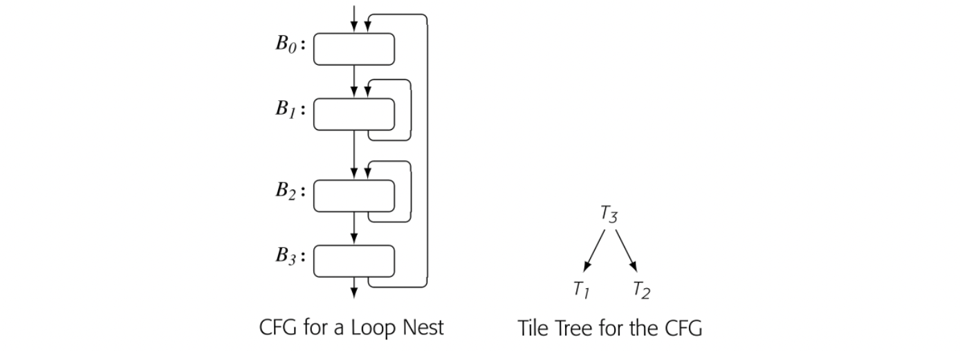
In this scheme, the allocator imposes a hierarchical model on the nodes of the CFG. In the model, a tile represents one or more CFG nodes and the flow between them. Tiles are chosen to encapsulate loops. In the CFG shown in the margin, tile $T_{1}$ consists of ${B_{1}}$ . Tile $T_{2}$ consists of ${B_{2}}$ . Tiles nest; thus, tile $T_{3}$ contains ${B_{0}, T_{1}, T_{2}, B_{3}}$ . The tile tree in the margin captures this relationship; $T_{1}$ and $T_{2}$ are siblings, as well as direct descendants of $T_{3}$ .

The hierarchical allocator performs control-flow analysis to discover loops and group blocks into tiles. To provide a concrete representation for the nesting among the tiles, it builds a tile tree in which subtiles are children of the tile that contains them.

Next, the hierarchical allocator performs a bottom-up walk over the tile tree. At each tile, $T_{i}$ , it builds an interference graph for the tile, performs coalescing, attempts to color the graph, and inserts spill code as needed. When it finishes with $γ_{i}$ , the allocator constructs a summary tile to represent $γ_{i}$ during the allocation of $γ_{i}$ 's parent. The summary tile takes on the LiveIn and LiveOut properties of the region that it represents, as well as the aggregate details of allocation in the region--the number of allocated registers and any PR preferences.

Once all the tiles have been individually colored, the allocator makes a top-down pass over the tile tree to perform assignment--that is, to map the allocation onto PRs. This pass follows the basic form of the global allocator, but it pays particular attention to values that are live across a tile boundary.

The bottom-up allocation pass discovers LRs one tile at a time. This process splits values that are live across tile boundaries; the allocator introduces copy operations for those splits. The split points isolate spill decisions inside a tile from register pressure outside a tile, which tends to drive spills to the boundaries of high-pressure tiles.

Of course, the allocator could run a postal- location coalescing pass over the allocated code.

Cross-tile connections between live ranges become copy operations. The allocator uses a preferencing mechanism similar to biased coloring to remove these copies where practical (see Section 13.5.1). The same mechanism lets the allocator model requirements for a specific PR.

Experiments suggest that the hierarchical allocator, with its shorter live ranges, produced slightly better allocations than a straightforward implementation of the global coloring allocator. Those same measurements showed that the allocator itself used more compile time than did the baseline global coloring allocator. The extra overhead of repeated allocation steps appears to overcome the asymptotic advantage of building smaller graphs.

13.6 Summary and Perspective

Because register allocation is an important part of a modern compiler, it has received much attention in the literature. Strong techniques exist for both local and global allocation. Because many of the underlying problems are NP-hard, the solutions tend to be sensitive to small decisions, such as how ties between identically ranked choices are broken.

Progress in register allocation has come from the use of paradigms that provide intellectual leverage on the problem. Thus, graph-coloring allocators have been popular, not because register allocation is identical to graph coloring, but rather because coloring captures some of the critical aspects of the global allocation problem. In fact, many of the improvements to coloring allocators have come from attacking the points where the coloring paradigm does not accurately reflect the underlying problem, such as better cost models and improved methods for live-range splitting. In effect, these improvements have made the paradigm more closely fit the real problem.

Chapter Notes

Register allocation dates to the earliest compilers. Backus reports that Best invented the algorithm from Section 13.3 in the mid-1950s for the original Fortran compiler [27, 28]. Best's algorithm has been rediscovered and reused in many contexts [39, 127, 191, 254]. It best-known incarnation is as Belady's offline page-replacement algorithm, Min[39]. Horwitz [208] and Kennedy [225] both describe the complications created by clean and dirty values. Liberatore et al. suggest spilling clean values before dirty values as a compromise [254].

The connection between graph coloring and storage-allocation problems was suggested by Lavrov [250] in 1961; the Alpha project used coloring to pack data into memory [151, 152]. Schwartz describes early algorithms by Ershov and by Cocke [320] that focus on using fewer colors and ignore spilling. The first complete graph-coloring allocator was built by Chaitin et al. for IBM's PL8 compiler [80, 81, 82].

The global allocator in Section 13.4 follows Chaitin's plan with Briggs' modifications [57, 58, 62]. It uses Chaitin's definition of interference and the algorithms for building the interference graph, for coalescing, and for handling spills. Briggs added an SSA-based algorithm for live range construction, an improved coloring heuristic, and several schemes for live-range splitting [57].

The treatment of register classes derives from Smith, Ramsey, and Holloway [331]. Chaitin, Nickerson, and Briggs all discuss achieving some of the same goals by adding edges to the interference graph to model specific assignment constraints [60, 82, 284].

The notion of coloring disjoint subgraphs independently follows from Smith, Ramsey, and Holloway. Earlier, Gupta, Soffa, and Steele suggested partitioning the graph into independent graphs using clique separators [184] and Harvey proposed splitting it between general purpose and floating-point registers [111].

Many improvements to the basic Chaitin-Briggs scheme have appeared in the literature and in practice. These include stronger coalescing methods [168, 289], better methods for spilling [40, 41], register scavenging [193], rematerialization of simple values [61], and live-range splitting [107, 116,244]. Register promotion has been proposed as a preallocation transformation that rewrites the code to increase the set of values that can be kept in a register [73, 77, 258, 261, 315]. DasGupta proposed a precise incremental update for coalescing and spilling, as well as a faster but somewhat lossy update [124]. Harvey looked at coloring spill locations to reduce spill memory requirements [193].

The SSA-based allocators developed from the independent work of several authors [64, 186, 292]. Both Hack and Bouchez built on the original observation with in-depth treatments [53, 185]. Linear scan allocation was proposed by Poletto and Sarkar [296]. The hierarchical coloring scheme is due to Koblenz and Callahan [75, 106].

Chapter 14. Runtime Optimization

ABSTRACT Runtime optimization has become an important technique for the implementation of many programming languages. The move from ahead-of-time compilation to runtime optimization lets the language runtime and its compilers capitalize on facts that are not known until runtime. If these facts enable specialization of the code, such as folding an invariant value, avoiding type conversion code, or replacing a virtual function call with a direct call, then the profit from use of runtime information can be substantial.

This chapter explores the major issues that arise in the design and implementation of a runtime optimizer. It describes the workings of a hot-trace optimizer and a method-level optimizer; both are inspired by successful real systems. The chapter lays out some of the tradeoffs that arise in the design and implementation of these systems.

KEYWORDS Runtime Compilation, Just-in-Time Compilation, Dynamic Optimization

14.1 Introduction

Runtime optimization code optimization applied at runtime

Many programming languages include features that make it difficult to produce high-quality code at compile time. These features include late binding, dynamic loading of both declarations and code (classes in JAVA), and various kinds of polymorphism. A classic compiler, sometimes called an ahead-of-time compiler (AOT), can generate code for these features. In many cases, however, it does not have sufficient knowledge to optimize the code well. Thus, the AOT compiler must emit the generic code that will work in any situation, rather than the tailored code that it might generate with more precise information.

For some problems, the necessary information might be available at link time, or at class-load time in JAVA. For others, the information may not be known until runtime. In a language where such late-breaking information can have a significant performance impact, the system can defer optimization or translation until it has enough knowledge to produce efficient code.

Compiler writers have applied this strategy, runtime optimization or just-in-time compilation (JIT), in a variety of contexts, ranging from early LISP systems through modern scripting languages. It has been used to build regular-expression search facilities and fast instruction-set emulators. This chapter describes the technical challenges that arise in runtime optimization and runtime translation, and shows how successful systems have addressed some of those problems.

Just-in-time compilers are, undoubtedly, the most heavily used compilers that the computer science community has built. Most web browsers include JITs for the scripting languages used in web sites. Runtime systems for languages such as JAVA routinely include a JIT that compiles the heavily used code. Because these systems compile the code every time it runs, they perform many more compilations than a traditional AOT compiler.

Conceptual Roadmap

Classic AOT compilers make all of their decisions based on the facts that they can derive from the source text of the program. Such compilers can generate highly efficient code for imperative languages with declarations. However, some languages include features that make it impossible for the compiler to know important facts until runtime. Such features include dynamic typing, some kinds of polymorphism, and an open class structure.

Runtime optimization involves a fundamental tradeoff between time spent compiling and code quality. The runtime optimizer examines the program's state to derive more precise information; it then uses that knowledge to specialize the executable code. Thus, to be effective, the runtime optimizer must derive useful information. It must improve runtime performance enough to compensate for the added costs of optimization and code generation. The compiler writer, therefore, has a strong incentive to use methods that are efficient, effective, and broadly applicable.

A Few Words About Time

Runtime optimization adds a new layer of complexity to our reasoning about time. These techniques intermix compile time with runtime and incur compile-time costs every time a program executes.

JIT time We refer to the time when the runtime opti- mizer or the just-in-time compiler is, itself, executing as JIT time.

At a conceptual level, the distinction between compile time and runtime remains. The runtime optimizer plans runtime behavior and runtime data structures, just as an AOT compiler would. It emits code to create and maintain the runtime environment. Thus, JIT-time activities are distinct from runtime activities. All of the reasoning about time from earlier chapters is relevant, even if the time frame when the activities occur has shifted.

To further complicate matters, some systems that use runtime optimization rely on an interpreter for their default execution mode. These systems interpret code until they discover a segment of code that should be compiled. At that point they compile and optimize the code; they then arrange for subsequent executions to use the compiled code for the segment. Such systems intermix interpretation, JIT compilation, and execution of compiled code.

Overview

To implement efficiently features such as late binding of names to types or classes, dynamic loading and linking of code, and polymorphism, compiler writers have turned to runtime optimization. A runtime optimizer can inspect the running program's state to discover information that was obscured or unavailable before runtime.

Runtime compilation also provides nat- ural mechanisms to deal with runtime changes in the program’s source text (see Section 14.5.4).

By runtime, the system mostly knows what code is included in the executable. Late bound names have been resolved. Data structures have been allocated, so their sizes are known. Objects have been instantiated, with full class information. Using facts from the program's runtime state, a compiler can specialize the code in ways that are not available to an AOT compiler.

Runtime compilation has a long history. McCarthy's early LISP systems compiled native code for new functions at runtime. Thompson's construction, which builds an NFA from a regular expression, was invented to compile an RE into native code inside the search command for the QED editor--one of the first well-known examples of a compiler that executed at runtime. Subsequent systems used these techniques for purposes that ranged from the implementation of dynamic object-oriented languages such as SMALLtalk-80 through code emulation for portability. The rise of the World Wide Web was, in part, predicated on widespread use of JAVA and JAVASCRIPT, both of which rely on runtime compilation for efficiency.

Runtime optimization presents the compiler writer with a novel set of challenges and opportunities. Time spent in the compiler increases the overall running time, so the JIT writer must balance JIT costs against expected improvement. Techniques that shift compilation away from infrequently executed, or cold, code and toward frequently executed, or hot, code can magnify any gain from optimization.

We use the term JIT to cover all runtime optimizers, whether their input is source code, as in McCarthy's early LISP systems; some high-level notation, as in Thompson's RE-to-native-code compiler; some intermediate form as in JAVA systems; or even native code, as in Dynamo. The digressions throughout this chapter will introduce some of these systems, to familiarize the reader with the long history and varied applications of these ideas.

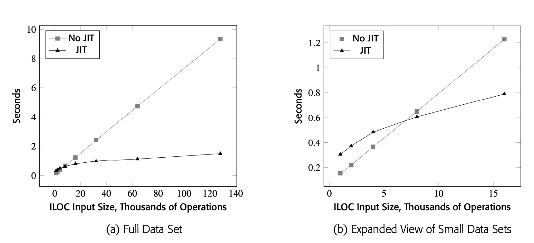
Impact of JIT Compilation

The data was gathered on OpenJDK version 1.8.0_292 running on an Intel ES2640 at 2.4GHz.

The input codes had uniform register pres- sure of 20 values. The allocator was allotted 15 registers.

JIT compilation can make a significant difference in the execution speed of an application. As a concrete example, Fig. 14 shows the running times of a JAVA implementation of the local register allocation algorithm from Section 13.3. Panel (a) shows the running time of the allocator on a series of blocks with 1,000 lines, 2,000 lines, 4,000 lines, and so on up to 128,000 lines of ILOC code. The gray line with square data points shows the running time with the JIT disabled; the black line with triangular data points shows the running time with the JIT enabled. Panel (b) zooms in on the startup behavior--that is, the smaller data sets.

These numbers are specific to this single application. Your experience will vary.

The JIT makes a factor of six difference on the largest data set; it more than compensates for the time spent in the JIT. Panel (a) shows the JIT's contribution to the code's performance. Panel (b) shows that VM-code emulation is actually faster on small data sets. Time spent in the JIT slows execution in the early stages of runtime; after roughly one-half second, the speed advantage of the compiled code outweighs the costs incurred by the JIT.

Roadmap

JIT design involves fundamental tradeoffs between the amount of work performed ahead of time, the amount of work performed in the JIT, and the improvement that JIT compilation achieves. As languages, architectures, and runtime techniques have changed, these tradeoffs have shifted. These tradeoffs will continue to shift and evolve as the community's experience with building and deploying JITs grows. Our techniques and our understanding will almost certainly improve, but the fundamental tradeoff of efficiency against effectiveness will remain.

This chapter provides a snapshot of the state of the field at the time of publication. Section 14.2 describes four major issues that play important roles in shaping the structure of a JIT-enabled system. The next two sections present high-level sketches for two JITs that sit at different points in the design space. Section 14.3 describes a hot-trace optimizer while Section 14.4 describes a hot-method optimizer; both designs are modeled after successful systems. The Advanced Topics section explores several other issues that arise in the design and construction of practical JIT-based systems.

14.2 Background

Runtime optimization has emerged as a technology that lets the runtime system adapt the executable code more closely to the context in which it executes. In particular, by deferring optimization until the compiler has more complete knowledge about types, constant values, and runtime behavior (e.g., profile information), a JIT compiler can eliminate some of the overhead introduced by language features such as object-orientation, dynamic typing, and late binding.

Success in runtime optimization, however, requires attention to both the efficiency and the effectiveness of the JIT. The fundamental principle of runtime optimization is

$A runtime compiler must save more cycles than it uses.$

If the runtime compiler fails to meet this constraint, then it actually slows down the application's execution.

This critical constraint shapes both the JIT and the runtime system with which it interacts. It places a premium on efficiency in the compiler itself. Because compile time now adds to running time, the JIT implementation's efficiency directly affects the application's running time. Both the scope and ambition of the JIT matter; both asymptotic complexity and actual runtime overhead matter. Equally important, the scheme that chooses which code segments to optimize has a direct impact on the total cost of running an application.

This constraint also places a premium on the effectiveness of each algorithm that the JIT employs. The compiler writer must focus on techniques that are both widely applicable and routinely profitable. The JIT should apply those techniques to regions where opportunities are likely and where those improvements pay off well. A successful JIT improves the code's running time often enough that the end users view time spent in the JIT as worthwhile.

Regular expression search in the QED editor Ken Thompson built a regular-expression (RE) search facility into the QED editor in the late 1960s. This search command was an early JIT compiler, invoked under the user's direction. When the user entered an RE, the editor invoked the JIT to create native code for the IBM 7094. The editor then invoked the native code to perform the search. After the search, it discarded the code.

The JIT was a compiler. It first parsed the RE to check its syntax. Next, it converted the RE to a postfix notation. Finally, it generated native code to perform the search. The JIT's code generator used the method now known as Thompson's construction to build, implicitly, an NFA (see Section 2.4.2). The generated code simulated that NFA. It used search to avoid introducing duplicate terms that would cause exponential growth in the runtime state.

The QED search command added a powerful capability to a text editor that ran on a 0.35 MIP processor with 32 KB of RAM. This early use of JIT technology created a responsive tool that ran in this extremely constrained environment.

This situation differs from that which occurs in an AOT compiler. Compiler writers assume that the code produced by an AOT compiler executes, on average, many times per compilation. Thus, the cost of optimization is a small concern. AOT compilers apply a variety of transformations that range from broadly applicable methods such as value numbering to highly specific ones such as strength reduction. They employ techniques that produce many small improvements and others that produce a few large improvements. An AOT compiler wins by accumulating the improvements from a suite of optimizations, used at every applicable point in the code. The end user is largely insulated from the cost of compilation and optimization.

To recap, the constraints in a JIT mean that the JIT writer must choose transformations well, implement them carefully, and apply them to regions that execute frequently. Fig. 14.1 demonstrates the improvement from JIT compilation with the HotSpot Server Compiler. In that test, HotSpot produced significant improvements for codes that ran for more than one-half of a second. Careful attention to both costs and benefits allows this JIT to play a critical role in JAVA's runtime performance.

14.2.1 Execution Model

The choice of an $execution model$ has a large impact on the shape of a runtime optimization system. It affects the speed of baseline execution. It affects the amount of compilation that the system must perform and, therefore,the cumulative overhead of optimization. It also affects the complexity of the implementation.

A runtime optimization system can be complex. It takes, as input, code for some virtual machine (VM) code. The VM code might be code for an abstract machine such as the JAVA VM (JVM) or the Smalltalk-80 VM. In other systems, the VM code is native machine code. As output, the runtime optimizer produces the results of program execution.

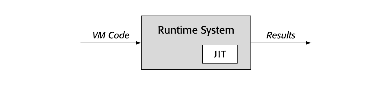
The difference between these modes is largely transparent to the user.

The runtime system can produce results by executing native code, by interpreting VM code, or by JIT compiling VM code to native code and running it. The relationship between the JIT, the code, and the rest of the runtime system determines the mode of execution. Does the system execute, by default, native code or VM code? Either option has strengths and weaknesses.

native-code execution usually implies JIT compilation before execution, unless the VM code is native code.
VM-code execution usually implies interpretation at some level. The code is compact; it can be more abstract than native code.

Native-code execution is, almost always, faster than VM-code execution. Native code relies on hardware to implement the fetch-decode-execute cycle, while VM emulation implements those functions in software. Lower cost per operation turns into a significant performance advantage for any nontrivial execution.

A VM-code system can defer scanning and parsing a procedure until it is called. The savings in startup time can be substantial.

On the other hand, VM-code systems may have lower startup costs, since the system does not need to compile anything before it starts to execute the application. This leads to faster execution for short-running programs, as shown in Fig. 14.1(b). For procedures that are short or rarely executed, VM-code emulation may cost less than JIT compilation plus native-code execution.

The Deutsch-Schiffman SMALLTALK-80 system used three formats for an AR.

It translated between formats based on whether or not the code accessed the AR as data.

The introduction of a JIT to a VM-code system typically creates a mixed-mode platform that executes both VM code and native code. A mixed-mode system may need to represent critical data structures, such as activation records, in both the format specified for the VM and the format supported by the native ISA. The dual representations may introduce translation between VM-code structures and native-code structures; those translations, in turn, will incur runtime costs.

ADAPTIVE FORTRAN Adaptive Fortran was a runtime optimizer for FORTRAN IV built by Hansen as part of the work for his 1974 dissertation. He used it to explore both the practicality and the profitability of runtime optimization. Adaptive Fortran introduced many ideas that are found in modern systems.

The system used a fast ahead-of-time compiler to produce an IR version of the program; the IR was grouped into basic blocks. At runtime, the IR was interpreted until block execution counts indicated that the block could benefit from optimization. (The AOT compiler produced block-specific, optimization-specific thresholds based on block length, nesting depth, and the cost of the JIT optimization.)

Guided by the execution counts and thresholds, a supervisor invoked a JIT to optimize blocks and their surrounding context. The use of multiple block-specific thresholds led to an effect of progressive optimization—more optimizations were applied to blocks that accounted for a larger share of the running time.

One key optimization, which Hansen called fusion, aggregated together multiple blocks to group loops and loop nests into segments. This strategy allowed Adaptive Fortran to apply loop-based optimizations such as code motion.

The alternative, native-code execution, distributes the costs in a different way. Such a system must compile all vm code to native code, either in an AOT compilation or at runtime. The AOT solution leads to fully general code and, thus, a higher price for nonoptimized native execution. The JIT solution leads to a system that performs more runtime compilation and incurs those costs on each execution.

There is no single best solution to these design questions. Instead, the compiler writer must weigh carefully a variety of tradeoffs and must implement the system with an eye toward both efficiency and effectiveness. Successful systems have been built at several points in this design space.

14.2.2 Compilation Triggers

The runtime system must decide when and where to invoke the JIT. This decision has a strong effect on overall performance because it governs how often the JIT runs and where the JIT focuses its efforts.

Runtime optimizers use JIT compilation in different ways. If the system JIT compiles all code, as happens in some native-code systems, then the trigger may be as simple as "compile each procedure before its first call." If, instead,the system only compiles hot code, the trigger may require procedure-level or block-level profile data. Native-code environments and mixed-mode environments may employ different mechanisms to gather that profile data.

In a native-code environment, the compiler writer must choose between (1) a system that works from VM code and compiles that VM code to native code before it executes, or (2) a system that works from AOT-compiled native code and only invokes the JIT on frequently executed, or hot, code. The two approaches lead to distinctly different challenges.

VM-Code Execution

In a mixed-mode environment, the system can begin execution immediately and gather profile data to determine when to JIT compile code for native execution. These systems tend to trigger compilation based on profile data exceeding a preset threshold value above which the code is considered hot. This approach helps the system avoid spending JIT cycles on code that has little or no impact on performance.

Threshold values play a key role in determining overall runtime. Larger threshold values decrease the number of JIT compilations. At the same time, they increase the fraction of runtime spent in the VM-code emulator, which is typically slower than native-code execution. Varying the threshold values changes system behavior.

Backward branch In this context, a backward branch or jump targets an address smaller than the program counter. Loop-closing branches are usually back- ward branches.

To obtain accurate profile data, a VM-code environment can instrument the application's branches and jumps. To limit the overhead of profile collection, these systems often limit the set of points where they collect data. For example, blocks that are the target of a backward branch are good candidates to profile because they are likely to be loop headers. Similarly, the block that starts a procedure's prolog code is an obvious candidate to profile. The system can obtain call-site specific data by instrumenting precall sequences. All of these metrics, and others, have been used in practical and effective systems.

Native-Code Execution

If the system executes native code, it must compile each procedure before that code can run. The system can trigger compilation at load time, either in batch for the entire executable (Speed Doubler) or as modules are loaded (early versions of the V8 system for JAVASCRIPT). Alternatively, the system can trigger the compiler to translate each procedure the first time it runs. To achieve that effect, the system can link a stub in place of any yet-to-be-compiled procedure; the stub locates the VM code for the callee, JIT compiles and links it, and reexecutes the call.

SPEED DOUBLER Speed Doubler was a commercial product from Connectix in the 1990s. It used load-time compilation to retarget legacy applications to a new ISA. Apple had recently migrated its Macintosh line of computers from the Motorola MC 68000 to the IBM POWER PC. Support for legacy applications was provided by an emulator built into the MacOS.

Speed Doubler was a load-time JIT that translated MC 68000 applications into native POWER PC code. By eliminating the emulation overhead, it provided a substantial speedup. When installed, it was inserted between the OS loader and the start of application execution. It did a quick translation, then branched to the application’s startup code.

The initial version of Speed Doubler appeared to perform an instruction-by- instruction translation, which provided enough improvement to justify the product’s name. Subsequent versions provided better runtime performance; we presume it was the result of better optimization and code generation. Speed Doubler used native-code execution with a compile-on-load discipline to provide a simple and transparent mechanism to improve running times. Users perceived that JIT compilation cost significantly less than the speedups that it achieved, so the product was successful.

Load-time strategies must JIT-compile every procedure, whether or not it ever executes. Any delay from that initial compilation occurs as part of the application’s startup. Compile-on-call shifts the cost of initial compilation later in execution. It avoids compiling code that never runs, but it does com- pile any code that runs, whether it is hot or cold.

Decreasing time in the JIT directly reduces elapsed execution time.

If the system starts from code compiled by an AOT compiler, it can avoid these startup compilations. The AOT compiler can insert the necessary code to gather profile data. It might also annotate the code with information that may help subsequent JIT compilations. A system that uses precompiled na- tive code only needs to trigger the optimizer when it discovers that some code fragment is hot—that is, the code consumes enough runtime to justify the cost of JIT compiling it.

Hot Traces A trace optimizer watches runtime branches and jumps to discover hot traces. Once a trace's execution count exceeds the preset hot threshold, the system invokes the jit to construct an optimized native-code implementation of the trace.

Trace optimizers perform local or regional optimization on the hot trace, followed by native-code generation including allocation and scheduling. Because a runtime trace may include calls and returns, this "regional" optimization can make improvements that would be considered interprocedural in an AOT compiler.

Hot Methods A method optimizer finds procedures that account for a significant fraction of overall running time by monitoring various counters. These counters include call counts embedded in the prolog code, loop iteration counts collected before backward branches, and call-site specific data gathered in precall sequences. Once a method becomes hot, the system uses a jit to compile optimized native code for the method. Because it works on the entire method, the optimizer can perform nonlocal optimizations, such as code motion, regional instruction scheduling, dead-code elimination, global redundancy elimination, or strength reduction. Some method optimizers also perform inline substitution. They might pull inline the code for a frequently executed call in the hot method. If most calls to a hot method come from one call site, the optimizer might inline the callee into that caller.

The choice of granularity has a profound impact on both the cost of optimizations and the opportunities that the optimizer discovers.

Assume a trace that has one entry but might have premature exits.

A trace optimizer might apply lvn to the entire trace to find redundancy, fold constants, and simplify identities. Most method optimizers use a global redundancy algorithm, which is more expensive but should find more opportunities for improvement.

Linear scan achieves some of the benefits of global allocation with lower cost than graph coloring.

A trace optimizer might use a fast local register allocator like the algorithm from Section 13.3. By contrast, a method optimizer must deal with control flow, so it needs a global register allocator such as the coloring allocator or the linear scan allocator (see Sections 13.4 and 13.5.3). Again, the tradeoff comes down to the cost of optimization against the total runtime improvement.

14.2.4 Sources of Improvement

A jit can discover facts that are not known before runtime and use those facts to justify or inform optimization. These facts can include profile information, object types, data structure sizes, loop bounds, constant values or types, and other system-specific facts. To the extent that these facts enable optimization that cannot be done in an AOT compiler, they help to justify runtime compilation.

THE DEUTSCH-SCHIFFMAN SMALLTALK-80 SYSTEM

The Deutsch-Schiffman implementation of Smalltalk-80 used JIT compilation to create a native-code environment on a system with a Motorola MC 68000-series processor. Smalltalk-80 was distributed as an image for the Smalltalk-80 virtual machine.

This system only executed native-code. The method lookup and dispatch mechanism invoked the JIT for any method that did not have a native-code body—a compile-on-call discipline.

The system gained most of its speed improvement from replacing VM emulation with native-code execution. It used a global method cache and was the first system to use inline method caches. The authors were careful about translating between VM structures and native-code structures, particularly activation records. The result was a system that was astonishing in its speed when compared to other contemporary Smalltalk-80 implementations on off-the-shelf hardware.

The system ran in a small-memory environment. (16MB of RAM was considered large at the time.) Because native code was larger than VM code by a factor of two to five, the system managed code space carefully. When the system needed to reclaim code space, it discarded native code rather than paging it to disk. This strategy, sometimes called throw-away code generation, was profitable because of the large performance differences between VM emulation and native-code execution, and between JIT compilation and paging to a remote disk (over 10 MBPS Ethernet).

In practice, runtime optimizers find improvement in a number of different ways. Among those ways are:

In the Deutsch-Schiffman system, native code was fast enough to compensate for the JIT costs.

Eliminate VM Overhead If the JIT operates in a mixed-mode environment, the act of translation to native code decreases the emulation overhead. The native code replaces software emulation with hardware execution, which is almost always faster. Some early JITs, such as Thompson's JIT for regular expressions in the QED editor, performed minimal optimization. Their benefits came, almost entirely, from elimination of VM overhead.
Improve Code Layout A trace optimizer naturally achieves improvements from code layout. As it creates a copy of the hot trace, the JIT places the blocks in sequential execution order, with some of the benefits ascribed to global code placement (see Section 8.6.2).

Dynamo, in particular, benefited from lin- earization of the traces.

In the compiled copy of the hot trace, the JIT can make the on-trace path use the fall-through path at each conditional branch. At the same time, any end-of-block jumps in the trace become jumps to the next operation, so the JIT can simply remove them.

Eliminate Redundancy Most JITs perform redundancy elimination. A trace optimizer can apply the LUN or SVN algorithms, which also perform constant propagation and algebraic simplification. Both algorithms have $O (1)$ cost per operation. A method optimizer can apply DVNT or a data-flow technique such as lazy code motion or a global value-numbering algorithm to achieve similar benefits. The costs of these algorithms vary, as do the specific opportunities that they catch (see Sections 10.6 and 10.3.1).
Reduce Call Overhead Inline substitution eliminates call overhead. A runtime optimizer can use profile data to identify call sites that it should inline. A trace optimizer can subsume a call or a return into a trace. A method optimizer can inline call sites into a hot method. It can also use profile data to decide whether or not to inline the hot method into one or more of its callers.

We do not know of a JIT that performs model-specific optimization. For machine-dependent problems such as instruction scheduling, the benefits might be significant.

Tailor Code to the System Because the results of JIT compilation are ephemeral--they are discarded at the end of the execution--the JIT can optimize the code for the specific processor model on which it will run. The JIT might tailor a compute-bound loop to the available SIMD hardware or the GPU. Its scheduler might benefit from model-specific facts such as the number of functional units and their operation latencies.

An AOT compiler might identify values that can impact JIT optimization and include methods that query those values.

Capitalize on Runtime Information Programs often contain facts that cannot be known until runtime. Of particular interest are constant, or unchanging, values. For example, loop bounds might be tied to the size of a data structure read from external media--read once and never changed during execution. The JIT can determine those values and use them to improve the code. For example, it might move range-checks out of a loop (see Section 7.3.3). In languages with late binding, type and class information may be difficult or impossible to discern in an AOT compiler. The JIT can use runtime knowledge about types and classes to tailor the compiled code to the runtime reality. In particular, it might convert a generic method dispatch to a class-specific call.

JIT compilation can impose subtle constraints on optimization. For example, traditional AOT optimization often focuses on loops. Thus, techniques such as unrolling, loop-invariant code motion, and strength reduction have all proven important in the AOT model. Hot-trace optimizers that exclude cyclic paths cannot easily duplicate those effects.

The Dynamo Hot-Trace Optimizer

The Dynamo system was a native-code, hot-trace optimizer for Hewlett-Packard's PA-8000 systems. The system's fundamental premise was that it could efficiently identify and improve frequently executed traces while executing infrequently executed code in emulation.

To find hot traces, Dynamo counted the executions of blocks that were likely start-of-trace candidates. When a block's count crossed a preset threshold (50), the JIT would build a trace and optimize it. Subsequent executions of the trace ran the compiled code. The system maintained its own software-managed cache of compiled traces.

Dynamo achieved improvements from local and superlocal optimization, from improved code locality, from branch straightening, and from linking traces into larger fragments. Its traces could cross procedure-call boundaries, which allowed Dynamo to optimize interprocedural traces.

Dynamo showed that JIT compilation could be profitable, even in competition with code optimized by an AOT compiler. Subsequent work by others created a Dynamo-like system for the IA-32 ISA, called DynamoRIO.

ILOC includes the tbl pseudooperation to record and preserve this kind of knowledge.

Control-flow optimizations, such as unrolling or cloning, typically require a control-flow graph. It can be difficult to reconstruct a CFG from assembly code. If the code uses a jump-to-register operation (jump in ILOC), it may be difficult or impossible to know the actual target. In an IR version of the code, such branch targets can be recorded and analyzed. Even with jump-to-label operations (jumpI in ILOC), optimization may obfuscate the control-flow to the point where it is difficult or impossible to reconstruct. For example, Fig. 12.17 on page 126 shows a single-cycle, software-pipelined loop that begins with five jump-to-label operations; reconstructing the original loop from the CFG in Fig. 12.17(b) is a difficult problem.

14.2.4 Building a Runtime Optimizer

JIT construction is an exercise in engineering. It does not require new theories or algorithms. Rather, it requires careful design that focuses on efficiency and effectiveness, and implementation that focuses on minimizing actual costs. The success of a JIT-based system will depend on the cumulative impact of individual design decisions.

The rest of this chapter illustrates the kinds of tradeoffs that occur in a runtime optimizer. It examines two specific use cases: a hot-trace optimizer, in Section 14.3, and a hot-method optimizer, in Section 14.4. The hypothetical hot-trace optimizer draws heavily from the design of the Dynamo system.

The hot-method optimizer takes its inspiration from the original HotSpot Server Compiler and from the Deutsch-Schiffman SMALLTALK-80 system. Finally, Section 14.5 builds on these discussions to examine some of the more nuanced decisions that a JIT designer must make.

Selection Review In JIT design, compiler writers must answer several critical questions. They must choose an execution model; will the system run unoptimized code in an emulator or as native code? They must choose a granularity for compilation, typical choices are traces and whole procedures (or methods). They must choose the compilation triggers that determine when the system will optimize (and reoptimize) code. Finally, compiler writers must understand what sources of improvement the JIT will target, and they must choose optimizations that help with those particular issues.

Throughout the design and implementation process, the compiler writer must weigh the tradeoffs between spending more time on JIT compilation and the resulting reduction of time spent executing the code. Each of these decisions can have a profound impact on the effectiveness of the overall system and the running time of an application program.

Review Questions

In a system that executes native code by default, how might the system create the profile data that it needs? How might the system provide that data to the JIT?
Eliminating the overhead of VM execution is, potentially, a major source of improvement. In what situations might emulation be more efficient than JIT compilation to native code?

14.3 Hot-Trace Optimization

In the classic execution model for compiled code, the processor reads operations and data directly from the address space of the running process. The drawing labeled "Normal Execution" in the margin depicts this situation. (It is a simplified version of Fig. 15.) The fetch-decode-execute cycle uses the processor's hardware.

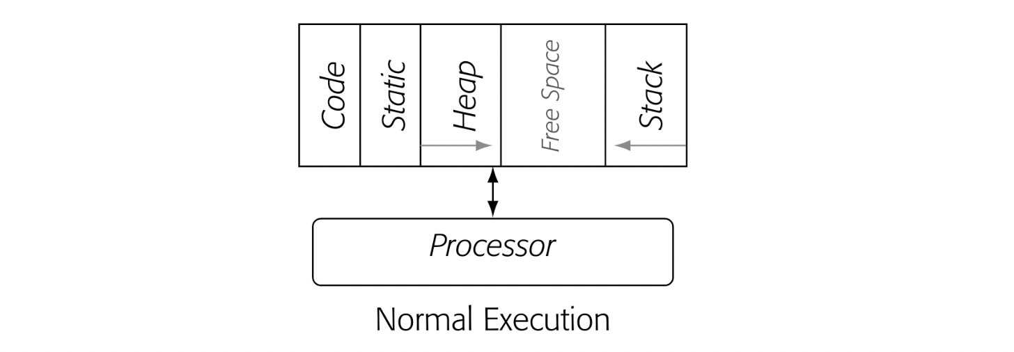
Conceptually, a native-code hot-trace optimizer sits between the executing process' address space and the processor. It "monitors" execution until it has "enough" context to determine that some portion of the code is hot and should be optimized. At that point, it optimizes the code and ensures that future executions of the optimized sequence run the optimized copy rather than the original code. The margin drawing depicts that situation.

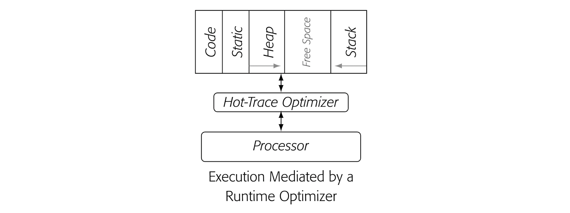
The hot-trace optimizer has a difficult task. It must find hot traces. It must improve those traces enough to overcome the costs of finding and compiling them. For each cycle spent in the jit, it must recover one or more cycles through optimization. In addition, if the process slows execution of the cold code, the optimized compiled code must also make up that deficit.

This section presents the design of a hot-trace optimizer. The design follows that of the Dynamo system built at Hewlett-Packard Research around the year 2000. It serves as both an introduction to the issues that arise and a concrete example to explore design tradeoffs.

Dynamo executed native code by emulation until it identified a hot trace. The emulator ran all of the cold code, gathered profile information, and identified the hot traces. Thus, emulated execution of the native code was slower than simply running that code on the hardware. The premise behind Dynamo was that improvement from optimizing hot traces could make up for both the emulation overhead and the jit compilation costs.

These design concepts raise several critical issues. How should the system define a trace? How can it find the traces? How does it decide a trace is hot? Where do optimized traces live? How does emulated cold code link to the hot code and vice versa?

14.3.1 Trace-Entry Blocks

In Dynamo, trace profiling, trace identification, and linking hot and cold code all depend on the notion of a trace-entry block. Each trace starts with an entry block. A trace-entry block meets one of two simple criteria. Either it is the target of a backward branch or jump, or it is the target of an exit from an existing compiled trace.

The first criterion selects blocks that are likely to be loop-header blocks. These blocks can be identified with an address comparison; if the target address is numerically smaller than the current program counter (PC), the target address designates a trace-entry block.

The second criterion selects blocks that may represent alternate paths through a loop. Any side exit from a trace becomes a trace-entry block. The jit identifies these blocks as it compiles a hot trace.

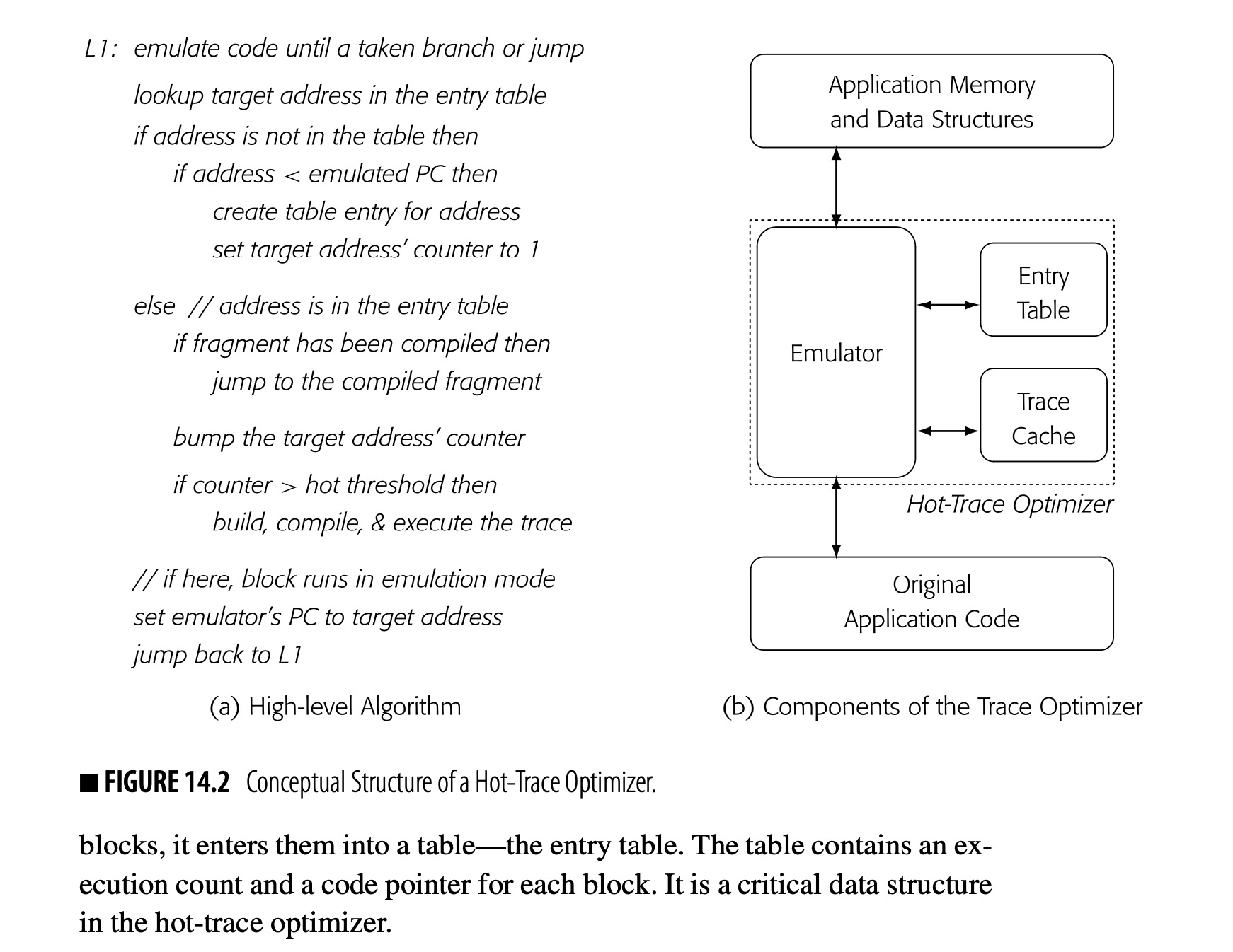
To identify and profile traces, the trace optimizer finds trace-entry blocks and counts the number of times that they execute. Limiting the number of profiled blocks helps keep overhead low. As the optimizer discovers entry blocks, it enters them into a table--the entry table. The table contains an execution count and a code pointer for each block. It is a critical data structure in the hot-trace optimizer.

14.3.1 Flow of Execution

Fig. 14.2(a) presents a high-level algorithm for the trace optimizer. The combination of the trace-entry table and the trace cache encapsulates the system's current state. The algorithm determines how to execute a block based on the presence or absence of that block in the entry table and the values of its execution counter and its code pointer.

Blocks run in emulation until they become part of a compiled hot trace. At that point, further executions of the compiled trace run the block as part of the optimized code. If control enters the block from another off-trace path, the block executes in emulation using the original code.

The critical set of decisions occurs when the emulator encounters a taken branch or a jump. (A jump is always taken.) At that point, the emulator looks for the target address in the trace entry table.

The smaller target address means that this branch or jump is a backward branch.

If the target address is not in the table and that address is numerically smaller than the current PC, the system classifies the target address as a trace entry block. It creates an entry in the table and initializes the entry’s execution counter to one. It then sets the emulator’s PC to the target address and continues emulation with the target block.
If, instead, the target address already has a table entry and that entry has a valid code pointer, the emulator transfers control to the compiled code fragment. Depending on the emulator’s implementation, discussed below, this transfer may require some brief setup code, similar to the precall sequence in a classic procedure linkage.

The compiled trace is stored in the trace cache.

Each exit path from the compiled trace either links to another compiled trace or ends with a short stub that sets the emulator’s PC to the address of the next block and jumps directly back to the emulator—to label $L 1$ in Fig. 14.2(a).

Section 14.3.2 discusses how the compiler can link compiled traces together.

If the target address is in the table but has not yet been compiled, the system increments the target address' execution counter and tests it against the hot threshold. If the counter is less than or equal to the threshold, the system executes the target block by emulation. When the target address' execution counter crosses the threshold, the system builds an IR image of the hot trace, executes and compiles that trace, stores the code into the trace cache, and stores its code pointer into the appropriate slot in the trace entry table. On exit from the compiled trace, execution continues with the next block. Either the code links directly to another compiled trace or it uses a path-specific exit stub to start emulation with the next block.

The algorithm in Fig. 14.2(a) shows the block-by-block emulation, interspersed with execution of optimized traces. The emulator jumps into optimized code; optimized traces exit with code that sets the emulator's PC and jumps back to the emulator. The rest of this section explores the details in more depth.

Emulation

Values that live in memory can use the same locations in both execution modes.

Following Dynamo, the trace optimizer executes cold code by emulation. The JIT-writer could implement the emulator as a full-fledged interpreter with a software fetch-decode-execute loop. That approach would require a simulated set of registers and code to transfer register values between simulated registers and physical registers on the transitions between emulated and compiled code. This transitional code might resemble parts of a standard linkage sequence.

As an alternative, the system could "emulate" execution by running the original compiled code for the block and trapping execution on a taken branch or jump. If hardware support for that trap is not available, the system can store the original operation and replace it with an illegal instruction--a trick used in debuggers since the 1960s.

When the PC reaches the end of the block, the illegal instruction traps. The trap handler then follows the algorithm from Fig. 14.2(a), using the stored operation to determine the target address. In this approach, individual blocks execute from native code, which may be faster than a software fetch-decode-execute loop.

Building the Trace

When a trace-entry block counter exceeds the hot threshold, the system invokes the optimizer with the address of the entry block. The optimizer must then build a copy of the trace, optimize that copy, and enter the optimized fragment into the trace cache.

While the system knows that the entry block has run more than threshold times, it does not actually know which path or paths those executions took. Dynamo assumes that the current execution will follow the hot path. Thus, the optimizer starts with the entry block and executes the code in emulation until it reaches the end of the trace--a taken backward branch or a transfer to the entry of a compiled trace. Again, comparisons of runtime addresses identify these conditions.

As the optimizer executes the code, it copies each block into a buffer. At each taken branch or jump, it checks for the trace-ending conditions. An untaken branch denotes a side exit from the trace, so the optimizer records the target address so that it can link the side exit to the appropriate trace or exit stub. When it reaches the end of the trace, the optimizer has both executed the trace and built a linearized version of the code for the JIT to optimize.

Consider the example shown in Fig. 14.3(a). When the emulator sees $B_{I}$ 's counter cross the hot-threshold, it invokes the optimizer. The optimizer executes $B_{I}$ and copies each of its operations into the buffer. The next branch takes control to $B_{2}$ ; the emulator executes $B_{2}$ and adds it to the buffer. Next, control goes to $B_{5}$ followed by $B_{6}$ . The branch at the end of $B_{6}$ goes back to $B_{I}$ , terminating the trace. At this point, the buffer contains $B_{I}$ , $B_{2}$ , $B_{5}$ , and $B_{6}$ , as shown in panel (b).

The drawing assumes that each of the side exits leads to cold code. Thus, the JIT builds a stub to handle each side exit and the end-of-trace exit. The stub labeled $B_{i}^{*}$ sets the emulator's pc to the start of block $B_{i}$ and jumps to the emulator. The stub also provides a location where the optimizer can insert any code needed to interface the compiled code with the emulated code. Panel (b) shows stubs for $B_{3}$ , $B_{4}$ , and $B_{7}$ .

The optimizer builds the trace based on the dynamic behavior of the executing code, which can produce complex effects. For example, a trace can extend through a procedure call and, with a simple callee, through a return. Because call and return are implemented with jumps rather than branches, they will not trigger the criteria for an exit block.

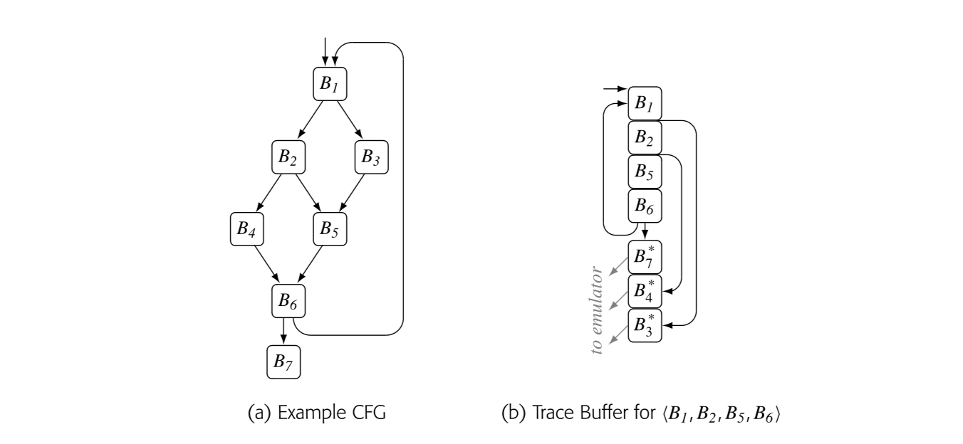extend through a procedure call and, with a simple callee, through a return. Because call and return are implemented with jumps rather than branches, they will not trigger the criteria for an exit block.

Optimizing the Trace

Once the optimizer has constructed a copy of the trace, it makes one or more passes over the trace to analyze and optimize the code. If the initial pass is a backward pass, the optimizer can collect Live information and other useful facts. From an optimization perspective, the trace resembles a single path through an extended basic block (see Section 8.5). In the example trace, an operation in $B_{6}$ can rely on facts derived from any of its predecessors, as they all must execute before control can reach this copy of $B_{6}$ .

The mere act of trace construction should lead to some improvements in the code. The compiler can eliminate any on-trace jumps. For each early exit, the optimizer should make the on-trace path be the fall-through path. This linearization of the code should provide a minor performance improvement by eliminating some branch and jump latencies and by improving instruction-cache locality.

The compiler writer must choose the optimizations that the JIT will apply to the trace. Value numbering is an obvious choice; it eliminates redundancies, folds constants, and simplifies algebraic identities.

If the trace ends with a branch to its entry block, the optimizer can unroll this path through the loop. In a loop with control flow, the result may be a loop that is unrolled along some paths and not along others--a situation that does not arise in a traditional AOT optimizer.

Early exits from the trace introduce complications. The same compensation-code issues that arise in regional scheduling apply to code motion across early exits (e.g., at the ends of $B_{I}$ and $B_{2}$ ). If optimization moves an operation across an exit, it may need to insert code into the stub for that exit.

Partially dead An operation is partially dead at point $p$ in the code if it is live on some paths that start at $p$ and dead on others.

The optimizer can detect some instances of dead or partially dead code. Consider an operation that defines $r_{i}$ . If $r_{i}$ is redefined before its next on-trace use, then the original definition can be moved into the stubs for any early exits between the original definition and the redefinition. If it is not redefined but not used in the trace, it can be moved into the stubs for the early exits and into the final block of the trace.

After optimization, the compiler should schedule operations and perform register allocation. Again, the local versions of these transformations can be applied, with compensation code at early exits.

Trace-Cache Size

The size of the trace cache can affect performance. Size affects multiple aspects of trace-cache behavior, from memory locality to the costs of lookups and managing replacements. If the cache is too small, the jtt may discard fragments that are still hot, leading to lost performance and subsequent re-compilations. If the cache is too large, it may retain code that has gone cold, hurting locality and raising lookup costs. Undoubtedly, compiler writers need to tune the trace-cache size to the specific system characteristics.

14.3.2 Linking Traces

One key to efficient execution is to recognize when other paths through the cfg become hot and to optimize them in a way that works well with the fragments already in the cache.

In the ongoing example, block $B_{I}$ became hot and the optimizer built a fragment for $⟨ B_{I}, B_{2}, B_{5}, B_{6} ⟩$ , as shown in Fig. 14.4(a). The early exits to $B_{3}$ and $B_{4}$ then make those blocks into trace-entry blocks. If $B_{3}$ becomes hot, the optimizer will build a trace for it. The only trace it can build is $⟨ B_{3}, B_{5}, B_{6} ⟩$ , as shown in panel (b).

If the optimizer maintains a small amount of information about trace entries and exits, it can link the two traces in panel (b) to create the code shown in panel (c). It can rewrite the branch to $B_{1}^{*}$ as a direct jump to $B_{1}$ . Similarly, it can rewrite the branch to $B_{3}^{*}$ as a direct jump to $B_{3}$ . The interlinked traces then create fast execution paths for both $⟨ B_{I}, B_{2}, B_{5}, B_{6} ⟩$ and $⟨ B_{I}, B_{3}, B_{5}, B_{6} ⟩$ , as shown in panel (c). The exits to $B_{4}$ and $B_{7}$ still run though their respective stubs to the interpreter. 1

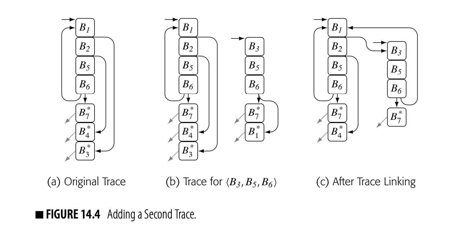
If during optimization of $⟨ B_{I}, B_{2}, B_{5}, B_{6} ⟩$ , the JIT moved operations into $B_{3}^{*}$ , then the process of linking would need to either (1) preserve $B_{3}^{*}$ on the path from $B_{I}$ to $B_{3}$ or (2) prove that the operations in $B_{3}^{*}$ are dead. With a small amount of context, such as the set of registers defined before use in the fragment, it could recognize dead compensation code in the stub.

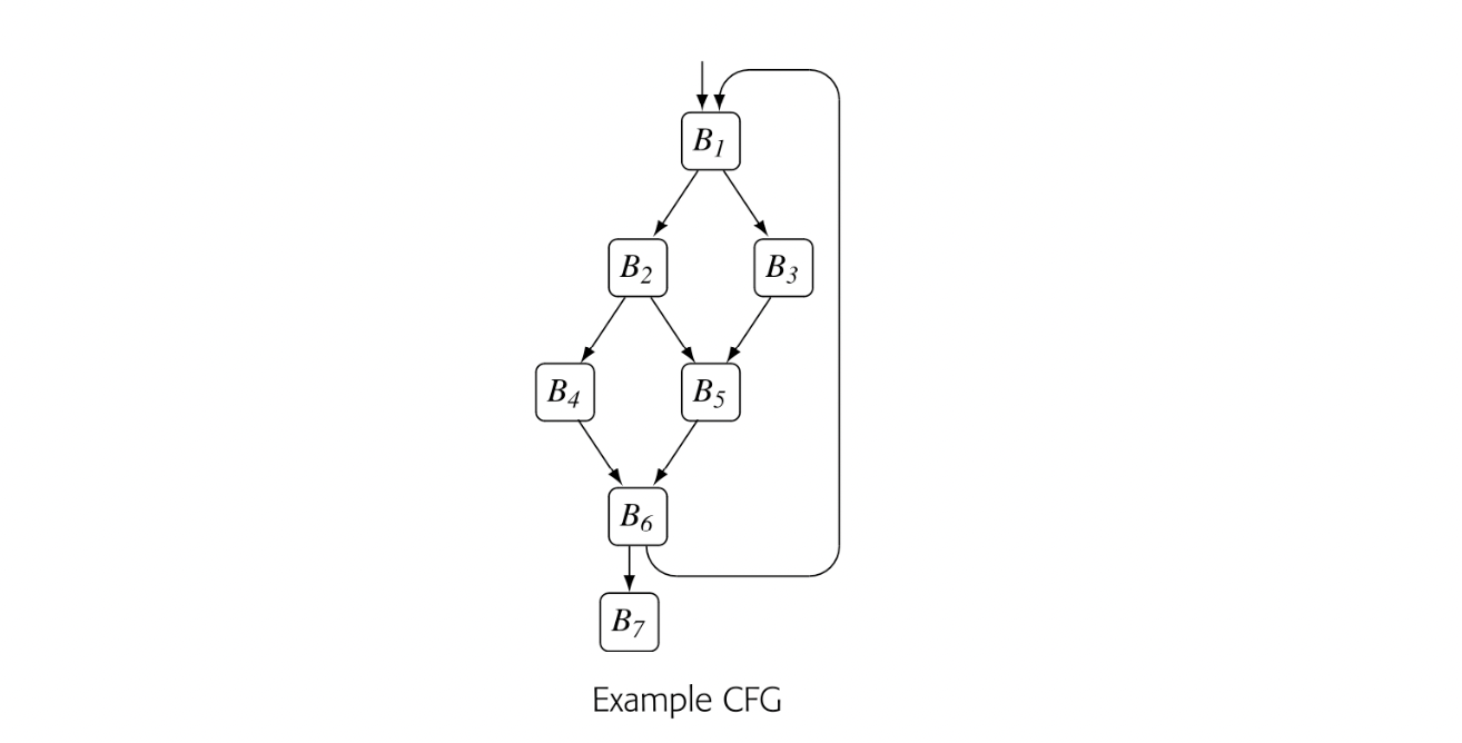
Cross-linking in this way also addresses a weakness in the trace-construction heuristic. The trace builder assumed that the $(k + 1)$ st execution of $B_{I}$ took the hot path. Because the system only instruments trace header blocks, $B_{I}$ 's execution count could have accrued from multiple paths between $B_{I}$ and $B_{6}$ . What happens if the $(k + 1)$ st execution takes the least hot of those paths?

With trace linking, the $(k + 1)$ st execution will build an optimized fragment. If that execution does not follow the hot path, then one or more of the early exits in the fragment will become hot; the optimizer will compile them and link them into the trace, capturing the hot path or paths. The optimizer will recover gracefully as it builds a linked set of traces.

Intermediate Entries to a Trace

In the example, when $B_{I}$ became hot, the system built an optimized trace for $⟨ B_{I}, B_{2}, B_{5}, B_{6} ⟩$ . When $B_{3}$ became hot, it optimized $⟨ B_{3}, B_{5}, B_{6} ⟩$ .

The algorithm, as explained, builds a single trace for $⟨ B_{I}, B_{2}, B_{5}, B_{6} ⟩$ and ignores the intermediate entry to the trace from the edge $(B_{3}, B_{5})$ . The system then executes the path $⟨ B_{3}, B_{5}, B_{6} ⟩$ by emulation until $B_{3}$ 's counter triggers compilation of that path. This sequence of actions produces two copies of the code for $B_{5}$ and $B_{6}$ , along with the extra JIT-time to optimize them.

Another way to handle the edge $(B_{3}, B_{5})$ would be to construct an intermediate entry into the trace $⟨ B_{I}, B_{2}, B_{5}, B_{6} ⟩$ . The trace-building algorithm, as explained, ignores these intermediate entry points, which simplifiesrecord-keeping. If the emulator knew that $B_{5}$ was an intermediate entry point, it could split the trace on entry $B_{5}$ . It would build an optimized trace for $⟨ B_{1}, B_{2} ⟩$ and another for $⟨ B_{5}, B_{6} ⟩$ . It would link the expected-case exit from $⟨ B_{1}, B_{2} ⟩$ to the head of $⟨ B_{5}, B_{6} ⟩$ .

$B_{4}$ has one predecessor while $B_{5}$ has two.

To implement trace splitting, the optimizer needs an efficient and effective mechanism to recognize an intermediate trace entry point--to distinguish, in the example, between $B_{4}$ and $B_{5}$ . The hot-trace optimizer, as described, does not build an explicit representation of the CFG. One option might be for the AOT compiler to annotate the VM code with this information.

Splitting $⟨ B_{1}, B_{2}, B_{5}, B_{6} ⟩$ after $B_{2}$ may produce less efficient code than compiling the unsplit trace. Splitting the trace avoids compiling $⟨ B_{5}, B_{6} ⟩$ a second time and storing the extra code in the code cache. It requires an extra slot in the entry block table. This tradeoff appears to be unavoidable. The best answer might well depend on the length of the common suffix of the two paths, which may be difficult to discern when compiling the first trace.

Selection Review

A hot-trace optimizer identifies frequently executed traces in the running code, optimizes them, and redirects future execution to the newly optimized code. It assumes that frequent execution in the past predicts frequent execution in the future and focuses the JIT's effort on such "hot" code. The acyclic nature of the traces leads to the use of local and superlocal optimizations. Those methods are fast and can capture many of the available opportunities.

The use of linked traces and interprocedural traces lets a hot-trace optimizer achieve a kind of partial optimization that an ahead-of-time compiler would not. The intent is to focus the JIT's effort where it should have maximum effect, and to limit its effort in regions where the expected impact is small.

Review Questions

Once a trace entry block becomes hot, the optimizer chooses the rest of the trace based on the entry-block's next execution. Contrast this strategy with the trace-discovery algorithm used in trace-scheduling. How might the results of these two approaches differ?
Suppose the trace optimizer fills its trace cache and must evict some trace. What steps would be needed to revert a specific trace so that it executes by VM-code emulation?

14.4 Hot-Method Optimization

Method-level optimization presents a different set of challenges and trade-offs than does trace-level optimization. To explore these issues, we will first consider a hot-method optimizer embedded in a JAVA environment. Our design is inspired by the original HotSpot Server Compiler (hereafter, HotSpot). The design is a mixed-mode environment that runs cold methods as JAVA bytecode and hot methods as native code. We finish this section with a discussion of the differences in a native-code hot-method optimizer.

14.4.1 Hot-Methods in a Mixed-Mode Environment

Fig. 14.5 shows an abstract view of the JAVA virtual machine or JVM. Classes and their associated methods are loaded into the environment by the Class Loader. Once stored in the VM, methods execute on an emulator--the figure's "Bytecode Engine." The JVM operates in a mixed-mode environment, with native-code implementations for many of the standard methods in system libraries.

To add a method-level JIT, the compiler writer must add several features to the JVM: the JIT itself, a software-managed cache for native-code method bodies, and appropriate interfaces. Fig. 14.6 shows these modifications.

From an execution standpoint, the presence of a JIT brings several changes. Cold code still executes via VM-code emulation; methods from native libraries still execute from native code. When the system decides that a method is hot, it JIT-compiles the VM code into native code and stores the 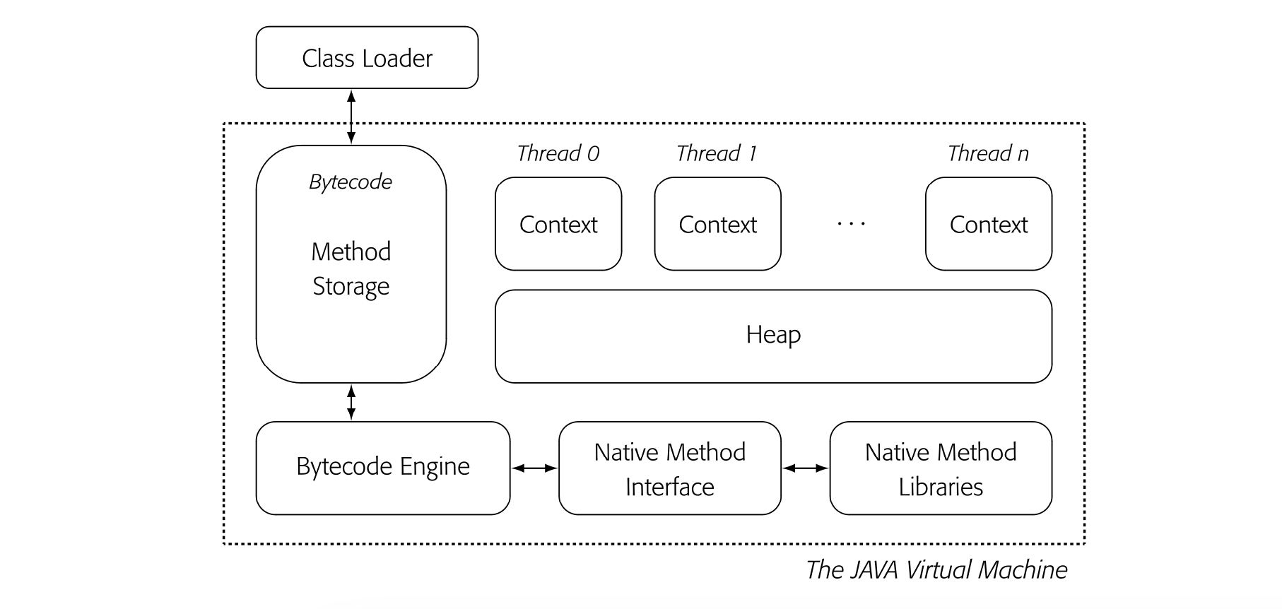new code in its native-code cache. Subsequent calls to that method run from the native code, unless the system decides to revert the method to VM-code emulation (see the discussion of deoptimization on page 742).

Using native-code ARs may necessitate translation between native-code and VM- code formats.

The JAVA community often refers to ARs as “stack frames.”

The compiler writer must make several key decisions. The system needs a mechanism to decide which methods it will compile. The system needs a strategy to gather profile information efficiently. The compiler writer must decide whether the native code operates on the VM-code or the native-code versions of the various runtime structures, such as activation records. The compiler writer must design and implement the JIT, which is just an efficient and constrained compiler. Finally, the compiler writer must design and implement a mechanism to revert a method to VM-code emulation when the compiled method proves unsuitable. We will explore these issues in order.

Trigger for Compilation

Conceptually, the hot-method optimizer should compile a method when that method consumes a significant fraction of the execution time. Finding a hot method that meets this criterion is harder than finding a hot trace, because the notion of a "significant fraction" of execution time is both imprecise and unknowable until the program terminates.

Iteration can occur with either loops or recursion. The mechanism should catch either case.

Thus, hot-method optimizers fall back on counters and thresholds to estimate a method's activity. This approach relies on the implicit assumption that a method that has consumed significant runtime will continue to consume significant runtime in the future. Our design, following HotSpot, will measure: (1) the number of times the method is called and (2) the number of times of loop iterations that it executes. Neither metric perfectly captures the notion that a method uses a large fraction of the running time. However, any method that does consume a significant fraction of runtime will almost certainly have a large value in one of those two metrics.

THE HOTSPOT SERVER COMPILER

Around 2000, Sun Microsystems delivered a pair of JITs for its JAVA environment: one intended for client-side execution and the other for server-side execution. The original HotSpot Server Compiler employed more expensive and extensive techniques than did the client-side JIT. The HotSpot Server compiler was notable in that it used strong global optimization techniques and fit them into the time and space constraints of a JIT. The authors used an IR that explicitly represented both control flow and data flow [92]. The IR, in turn, facilitated redundancy elimination, constant propagation, and code motion. Sparsity in the IR helped make these optimizations fast.

The JIT employed a novel global scheduling algorithm and a full coloring allocator (see Section 13.4). To make the coloring allocator practical, the authors developed a method to trim the interference graph that significantly shrank the graph. The result was a state-of-the-art JIT that employed algorithms once thought to be too expensive for use in a JIT.

The system can “sum” the counters by using a single location for all the counters in a method.

Thus, the system should count both calls to a method and loop iterations within a method. Strategically placed profile counters can capture each of these conditions. For call counts, the system can insert a profile counter into each method's prolog code. For iteration counts, the system can insert a profile counter before each loop-closing branch. To trigger compilation, it can either use separate thresholds for loops and invocations, or it can sum the counters and use a single threshold.

HotSpot counted both calls and iterations and triggered a compilation when the combined count exceeded a preset threshold of 10,000 events. This threshold is much larger than the one used in Dynamo (50). It reflects the more aggressive and expensive compilation in HotSpot.

Runtime Profile Data

To capture profile data, compiler writers can instrument either the VM code for the application or the implementation of the VM-code engine.

Instrumented VM Code. The system can insert VM code into the method to increment and test the profile counters. In this design, the profile overhead executes as VM code. Either the AOT compiler or the Class Loader can insert the instrumentation. Counter for calls can be placed in the method's prolog code, while counters for a specific call-site can be placed in the appropriate precall sequence.

To profile loop iterations, the transformation can insert a counter into any block that is the target of a backward branch or jump. An AOT strategy might decrease the cost of instrumentation; for example, if the AOT compiler knows the number of iterations, it can increment the profile counter once for the entire loop.

Instrumented Engine. The compiler writer can embed the profile support directly into the implementtaion of the VM-code engine. In this scheme, the emulator's code for branches, jumps, and the call operation (e.g., the JVM's invokestatic or invokevirtual) can directly increment and test the appropriate counters, which are stored at preplanned locations. Because the profile code executes as native code, it should be faster than instrumenting the VM code.

By contrast, an AOT compiler would find loop headers using dominators (see Sec- tion 9.2.1).

The emulator could adopt the address comparison strategy of the trace optimizer to identify loop header blocks. If the target address is numerically smaller than the PC, the targeted block is a potential loop header. Alternatively, it could rely on the AOT compiler to provide an annotation that identifies loop-header blocks.

Compiling the Hot Method

Tree-pattern matching techniques are a good match to the constraints of a JIT (see Section 11.4).

When profile data triggers the JIT to compile some method $x$ , the JIT can simply retrieve the VM code for $x$ and compile it. The JIT resembles a full-fledged compiler. It parses the VM code into an IR, applies one or more passes of optimization to the IR, and generates native code--performing instruction selection, scheduling, and register allocation. The JIT writes that native code into the native-code cache (see Fig. 14.6). Finally, it updates the tables or pointers that the system uses to invoke methods so that subsequent calls map to the cached native code.

In a mixed-mode environment, the benefits of JIT compilation should be greater than they are in a native-code environment because the cold code executes more slowly. Thus, a hot-method optimizer in a mixed-mode environment can afford to spend more time per method on optimization and code generation. Hot-method optimizers have applied many of the classic scalar optimizations, such as value numbering, constant propagation, dead-code elimination, and code motion (see Chapters 8 and 10). Compiler writers choose specific techniques for the combination of compile-time efficiency and effectiveness at improving code.

Global value numbering

The literature on method-level JITs often mentions global value numbering as one of the key optimizations that these JITs employ. The dutiful student will find no consensus on the meaning of that term. Global value numbering has been used to refer to a variety of distinct and different algorithms.

One approach extends the ideas from local value numbering to a global scope, following the path taken in superlocal and dominator-based value numbering (DVNT). These algorithms are more expensive than DVNT and the cost-benefit tradeoff between DVNT and the global algorithm is not clear.

Another approach uses Hopcroft's partitioning algorithm to find operations that compute the same value, and then rewrites the code to reflect those facts. The HotSpot Server compiler used this idea, which fit well with its program dependence graph IR.

Finally, the JIT writer could work from the ideas in lazy code motion (LCM). This approach would combine code motion and redundancy elimination. Because LCM implementations solve multiple data-flow analysis problems, the JIT writer would need to pay close attention to the cost of analysis.

Optimizations

Hot-method JITs apply local, regional, and global optimizations. Because the JIT operates at runtime, the compiler writer can arrange for an optimization to access the runtime state of the executing program to obtain runtime values and use them in optimization.

Value Numbering Method-level JITs typically apply some form of value numbering. It might be a regional algorithm, such as DVNT, or it might be one of a number of distinct global algorithms.

Value numbering is attractive to the JIT writer because these techniques achieve multiple effects at a relatively low cost. Typically, these algorithms perform some subset of redundancy elimination, code motion, constant propagation, and algebraic simplification.

Inline method caches can provide site- specific data about receiver types. The idea can be extended to capture type information on parameters, as well.

Specialization to Runtime Data A JIT can have access to data about the code's behavior in the current execution, particularly values of variables, type information, and profile data. Runtime type information lets the JIT speculate; given that a value consistently had type $t$ in the past, the JIT assumes that it will have type $t$ in the future.

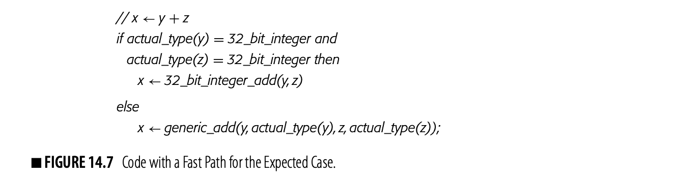
Such speculation can take the form of a fast-path/slow-path implementation. Fig. 14.7 shows, conceptually, how such a scheme might work. The code assumes that $x$ and $y$ are both 32-bit integers and tests for that case;if the test fails, it invokes the generic addition routine. If the slow path executes too many times, the system might recompile the code with new speculated types (see the discussion of "deoptimization" on page 742).

Inline Substitution The JIT can inline calls, which lets it eliminate method lookup overhead and call overhead. Inlining leads the JIT to tailor the callee's body to the environment at the call site. The JIT can use data from inline method caches to specialize code based on call-site specific type data. It can also inline call sites in the callee; it should have access to profile data and method cache data for all of those calls.

When a JIT considers inline substitution, it has access to all of the code for the applica- tion. In an AOT compiler, that situation is unlikely.

The JIT can also look back to callers to assess the benefits of inlining a method into one or more of its callers. Again, profile data on the caller and type information from the inline cache may help the JIT make good decisions on when to inline.

Code Generation Instruction selection, scheduling, and register allocation can each further improve the JIT-compiled code. Effective instruction selection makes good use of the ISA's features, such as address modes. Instruction scheduling takes advantage of instruction-level parallelism and avoids hardware stalls and interlocks. Register allocation tries to minimize expensive spill operations.

The challenge for the JIT writer is to implement these passes efficiently. Tree-pattern matching techniques for selection combine locally optimal code choice with extreme JIT-time efficiency. Both the scheduler and the allocator can capitalize on sparsity to make global algorithms efficient enough for JIT implementation. The HotSpot Server Compiler demonstrated that efficient implementations can make these global techniques not only acceptable but advantageous.

As with any JAVA system, a JIT should also try to eliminate null-pointer checks, or move them to places where they execute less frequently. Escape analysis can discover objects whose lifetimes are guaranteed to be contained within the lifetime of some method. Such objects can be allocated in the method's AR rather than on the heap, with a corresponding decrease in allocation and collection costs. Final and static methods can be inlined.

Deoptimization

Deoptimization the JIT generates less optimized code due to changes in runtime information

If the JIT uses runtime information to optimize the code, it runs the risk that changes in that data may render the compiled code either badly optimized or invalid. The JIT writer must plan for reasonable behavior in the event of a failed type speculation. The system may decide to deoptimize the code.

To “notice,” the system would need to in- strument the slow path.

Consider Fig. 14.7 again. If the system noticed, at some point, that most executions of this operator executed the generic_odd path, it might recompile the code to speculate on another type, to speculate on multiple types, or to not speculate at all. If the change in behavior is due to a phase-shift in program behavior, reoptimization may help.

If, however, the statement has simply stopped showing consistency in the types of $x, y$ , or $z$ , then repeated reoptimization may be the wrong answer. Unless the compiled code executes enough to cover the cost of JIT compilation, the recompilations will slow down execution.

The alternative is to deoptimize the code. Depending on the precise situation and the depth of knowledge that the JIT has about temporal type locality, it might use one of several strategies.

If the JIT knows that the actual type is one of a small number, it could generate fast path code for each of those types.
If the JIT knows nothing except that the speculated type is often wrong, it might generate unoptimized native code that just calls generic_odd or it might inline generic_odd at the operation.
If the JIT has been called too often on this code due to changing patterns, it might mark the code as not fit for JIT compilation, forcing the code to execute in emulation.

A deoptimization strategy allows the JIT to speculate, but limits the downside risk of incorrect speculation.

14.4.2 Hot-Methods in a Native-Code Environment

Several issues change when the JIT writer attempts hot-method optimization in a native-code environment. This section builds on insights from the Deutsch-Schiffman SMALLtalk-80 implementation.

Initial Compilations

The native-code environment must ensure that each method is compiled to native code before it runs. Many schemes will work, including a straightforward AOT compilation, load-time compilation of all methods, or JIT compilation on the first invocation, which we will refer to as compile oncall. The first two options are easier to implement than the last one. Neither, however, creates the opportunity to use runtime information during that initial compilation.

Using an indirect pointer to the code body (a pointer to a pointer) may simplify the implementation.

A compile-on-call system will first generate code for the program's main routine. At each call site, it inserts a stub that (1) locates the VM code for the method; (2) invokes the JIT to produce native code for the method; and (3) relinks the call site to point to the newly compiled native code. When the execution first calls method $m$ , it incurs a delay for the JIT to compile $m$ and then executes the native-code version of $m$ . If runtime facts are known, the first call to $m$ can capitalize on them.

If the JIT compiler supports multiple levels of optimization, the compiler writer must choose which level to use in these initial compiles. A lower level of optimization should reduce the cost of the initial JIT compiles, at the cost of slower execution. A higher level of optimization might increase the cost of the initial JIT compiles, with the potential benefit of faster execution.

To manage this tradeoff, the system may use a low optimization level in the initial compiles and recompile methods with a higher level of optimization when they become hot. This approach, of course, requires data about execution frequencies and type locality.

Gathering Profile Data

In a native-code environment, the system can gather profile information in two ways: instrument the code to collect profile data at specific points in the code, or shift to interrupt-driven techniques that discover where the executable spends its time.

Instrumented Code. The JIT compiler can instrument code as described earlier for a mixed-mode hot-method optimizer. The JIT can insert code into method prologs to count total calls to the method. It can obtain call-site specific counts by adding code to precall sequences. It can insert code to count loop iterations before loop-closing branches.

With instrumented code, JIT invocation proceeds in the same way that it would in the mixed-mode environment. The JIT is invoked when execution counts, typically call counts and loop iterations, pass some preset threshold. For a loop-iteration count, the code to test the threshold and trigger compilation should be inserted, as well.

To capture opportunities for type speculation and type-based code specialization, the JIT can arrange to record the type or class of specific values--typically, parameters passed to the method or values involved at a call in the method. The JIT should have access to that information.

Interrupt-Driven Profiles Method-invocation counts tell the system how often a method is called. Iteration counts tell the system how often a loop body executes. Neither metric provides insight into what fraction of total running time the instrumented code actually uses.

The system must produce tables to map an address into a specific location in the original code.

A native-code environment spends virtually all of its time executing application code. Thus, it can apply another strategy to discover hot code: interrupt-driven profiling. In this approach, the system periodically stops execution with a timer-driven interrupt. It maps the program-counter address at the time of the interrupt back to a specific method, and increments that method's counter. Comparing the method's counter against the total number of interrupts provides an approximation to the fraction of execution time spent in that method.

Some systems have used a combination of instrumented code and interrupt-driven profile data.

Because an interrupt-driven profile measures something subtly different than instrumented code measures, the JIT writer should expect that an interrupt-driven scheme will optimize different methods than an instrumented code scheme would.

The JIT still needs data, when possible, on runtime types to guide optimization. While some such data might exist in inline method caches at call sites, the system can only generate detailed information if the compiler adds type-profiling code to the executable.

Deoptimization with Native Code

When a compiled method begins execution, it must determine if the preconditions under which it was compiled (e.g., type or class speculation, constant valued parameters, etc.) still hold. The prolog code for a method can test any preconditions that the JIT assumed in its most recent compilation. In a mixed-mode environment, the system could execute the VM code if the precondition check fails; in a native-code environment, it must invoke the JIT to recompile the code in a way that allows execution to proceed.

In a recompilation, the system should attempt to provide efficient execution while avoiding situations where frequent recompilations negate the benefits of JIT compilation. Any one of several deoptimization strategies might make sense.

This strategy suggests a counter that limits the number of “phase shifts” the JIT will tolerate on a given method.

The JIT could simply recompile the code with the current best runtime information. If the change in preconditions was caused by a phase shift in program behavior, the current preconditions might hold for some time.
If the JIT supports multiple levels of optimization--especially with regard to type speculation--the system could instruct the JIT to use a lower level of speculation, which would produce more generic and lesstailored code. This approach tries to avoid the situation where the code for some method oscillates between two or more optimization states.
An aggressive JIT could compile a new version of the code with the current preconditions and insert a stub to choose among the variant code bodies based on preconditions. This approach trades increased code size for the possibility of better performance.

The best strategy will depend on how aggressively the JIT uses runtime information to justify optimizations and on the economics of JIT compilation. If the JIT takes a small fraction of execution time, the JIT writer and the user may be more tolerant of repeated compilations. By contrast, if it takes multiple invocations of a method to compensate for the cost of JIT compilation, then repeated recompilations may be much less attractive than lowering the level of speculation and optimization.

The Economics of JIT Compilation

The fundamental tradeoff for the JIT writer is the difference between cycles spent in the JIT and cycles saved by the JIT. In a native-code environment, the marginal improvement from the JIT may be lower, simply because the unoptimized code runs more quickly than it would in a similar mixed-mode environment.

This observation, in turn, should drive some of the decisions about which optimizations to implement and how much recompilation to tolerate. The JIT writer must balance costs, benefits, and policies to create a system that, on balance, improves runtime performance.

Section Review

A hot-method optimizer finds procedures that either execute frequently or occupy a significant fraction of execution time. It optimizes each procedure in light of the runtime facts that it can discern. Because a method optimizer can encounter control flow, it can benefit from regional and global optimizations, such as global value numbering or code motion; these transformations have higher costs and, potentially, higher payoffs than the local and superlocal techniques available to a trace optimizer.

The tradeoffs involved in a specific design depend on the execution environment, the source-language features that produce inefficiency, and the kinds of information gathered in the runtime environment. The design of a hot-method optimizer requires an understanding of the language, the system, the algorithms, and the behavior of the targeted applications.

14.5 Advanced Topics

The previous sections introduce the major issues that arise in the design of a runtime optimizer. To build such a system, however, the compiler writer must make myriad design decisions, most of which have an impact on the effectiveness of the system. This section explores several major topics that arise in the literature that surrounds jit compilation. Each of them has a practical impact on system design. Each of them can change the overall efficacy of the system.

14.5.1 Levels of Optimization

In practice, we know few developers who consider compile time when selecting an optimization level.

AOT compilers typically offer the end user a choice among multiple levels of optimization. This feature allows the user, in theory, to use stronger optimization in places where it matters, while saving on compile time in places where the additional optimization makes little difference.

A jit-based system might provide multiple levels of optimization for several reasons.

Because the elapsed time for application execution includes the jit's execution, the jit writer may decide to include in the standard compilation only those optimizations that routinely produce improvements.
The system may find that a native-code fragment executes often enough to justify more extensive analysis and optimization, which requires more jit time and saves more runtime.
If the jit performs speculation based on runtime information, such as types and classes, the jit may later need to deoptimize the code, which suggests a lower level of optimization.

For all these reasons, some runtime optimization systems have implemented multiple levels of optimization.

If the system discovers a loop with a large iteration count, it might apply loop-specific optimizations, such as unrolling, strength reduction, or code motion. To ensure that those changes have immediate effect, it could perform on-stack replacement (see Section 14.5.2).

If the system finds that one method accounts for a significant fraction of interrupt-based profile points, it might apply deeper analysis and more intense optimization. For example, it might inline calls, perform analyses to disambiguate types and classes, and reoptimize.

In either of these scenarios, a JIT with multiple levels of optimization needs a clear set of policies to govern when and where it uses each level of optimization. One key part of that strategy will be a mechanism to prevent the JIT from trying to change the optimization level too often--driving up the JIT costs without executing the code enough to amortize the costs.

14.5.2 On-Stack Replacement

A method-level JIT can encounter a situation in which one of the profile counters crosses its threshold during an execution of a long-running method. For example, consider a method with a triply nested loop that has iteration counts of 100 at each level. With a threshold of 10,000, the counter on the inner loop would trigger compilation after just one percent of the iterations.

In effect, the system behaves as if a long- running method has a higher threshold to trigger compilation.

The counter shows that the method is hot and should be optimized. If the system waits until the next call to "install" the optimized code, it will run the current code for the rest the current invocation. In the triply nested loop, the code would run 99 percent of the iterations after the counter had crossed the threshold for optimization.

To avoid this missed opportunity, the system could pause the execution, optimize and compile the code, and resume the execution with the improved code. This approach capitalizes on the speed of the compiled code for the majority of the loop iterations. To resume execution with the newly optimized code, however, the system must map the runtime state of the paused execution into the runtime state needed by the newly optimized code.

On-stack code replacement A technique where the runtime system pauses execution, JIT compiles the execut- ing procedure, and resumes execution with the newly compiled code

This approach, optimizing the procedure in a way that the current invocation can continue to execute, is often called on-stack code replacement. The JIT builds code that can, to the extent possible, execute in the current runtime environment. When it cannot preserve the values, it must arrange to map values from the current environment into the new environment.

The JIT can use its detailed knowledge of the old code to create the new environment. It can generate a small stub to transform the current environment--values in registers plus the current activation record--into the environment need by the new code.

The stub may need to move some values. The storage map of the new code may not match the storage map of the old code.
The stub may need to compute some values. Optimizations such as code motion or operator strength reduction may create new values that did not exist in the original code.
The stub may be able to discard some values. The state of the original code may contain values that are dead or unused in the new code.

The stub runs once, before the first execution of the new code. At that point, it can be discarded. If the jit runs in a separate thread, as many do, the system needs some handshaking between the jit and the running code to determine when it should switch to the new code.

The compiler writer has several ways to reduce the complexity of on-stack replacement.

She can limit the number of points in the code where the system can perform replacement. The start of a loop iteration is a natural location to consider. Execution of the next iteration begins after compilation and state mapping.

Techniques that create compensation code or introduce new values can complicate the mapping. Examples include code motion, software pipelining, and inline substitution.

She can simplify the state-mapping problem by limiting the set of optimizations that the jit uses when compiling for on-stack replacement. In particular, the jit might avoid techniques that require significant work to map the old environment into the new one.

The implementation of on-stack replacement ties in a fundamental way to the interfaces between emulated and compiled codes and their runtime environments. The details will vary from system to system. This strategy has the potential to provide significant improvement in the performance of long-running methods.

14.5.3 Code Cache Management

To avoid confusion, we will refer to the JIT’s cache as a $co d e c a c h e$ and to processor caches as hardware caches.

Almost all jit-based systems build and maintain a code cache--a dedicated, software-managed block of memory that holds jit-compiled code. The jit writer must design policies and build mechanisms to manage the code cache. Conceptually, code caches blend the problems and policies of a hardware cache and a software-managed heap.

Hardware caches determine an object's placement by an arithmetic mapping of virtual addresses to physical addresses. In a heap, software searches for a block of free space that will hold the object. Code caches are closer to the heap model for placement.
Hardware caches deal with fixed sized blocks. Heaps deal with requests for arbitrarily sized blocks, but often round those requests to some common sizes. Code caches must accommodate blocks of native code of different sizes.
Hardware caches use automatic, policy-based eviction schemes, typically informed by the pattern of prior use. Heaps typically run a collection phase to find blocks that are no longer live (see Section 6.6.2). Code caches use policies and mechanisms similar to hardware caches.

Most JIT-based systems have a separate code cache for each process or each thread. Some JIT writers have experimented with a global code cache, to allow the reuse of JIT compiled code across processes. The primary benefit from these designs appears to be a reduction in overall memory use; they may provide better performance for a multitasked environment on a limited memory system. When these systems find cross-process sharing, they also avoid reinvoking the JIT on previously compiled code, which can reduce overall runtimes.

If virtual memory is fast enough, the system can make the cache large and let the paging algorithms manage the problem.

The use of a limited-size code cache suggests that the standard virtual-memory paging mechanism is either too slow or too coarse-grained to provide efficient support for the JIT-compiled code. Use of a limited-size cache also implies that a code-cache eviction will discard the JIT-compiled code; delimiting it from the executing program and necessitating either emulation or a recompilation if it is invoked in the future.

Replacement Algorithm

When the JIT compiles code, it must write that code into the code cache. If the cache management software cannot find a block of unused memory large enough to hold the code, it must evict another segment from the cache.

A direct-mapped hardware cache has a set size of one.

Replacement in the code cache differs from replacement in a hardware cache. A set-associative hardware cache determines the set to which the new block maps and evicts one of the set's blocks. The literature suggests evicting the least recently used (Lru) block; many hardware caches use or approximate Lru replacement.

Code cache management algorithms need to evict enough segments to create room for the newly compiled code. In a hardware cache, eviction involves a single fixed-size line. In a software-managed code cache, allocation occurs at the granularity of the segment of compiled code (a trace, a method, or multiple methods). This complicates both the policy and the implementation of the replacement algorithm.

The cache management software should evict from the code cache one or more segments that have not been used recently. The evicted segmentsmust free enough space to accommodate the new code without wasting "too much" space. Choosing the LRU segment might be a good start, but the potential need to evict multiple segments complicates that decision. If the new code requires eviction of multiple segments, those segments must be adjacent. Thus, implementing an LRU mechanism requires some additional work.

The final constraint on replacement is that the algorithms must be fast; any time spent in the replacement algorithms adds to the application's running time. Creative engineering is needed to minimize the cost of choosing a block to evict and of maintaining the data structures to support that decision.

Fragmentation

Repeated allocation and replacement can fragment the space in a code cache. Collected heaps address fragmentation with compaction; uncollected heaps try to merge adjacent free blocks. Code caches lack the notion of a free command; in general, it is unknowable whether some code fragment will execute in the future, or when it will execute.

If the system executes in a virtual-memory environment, it can avoid some of the complication of managing fragmentation by using more virtual address space than allocated memory. As long as the code cache's working set remains within the intended cache size, the penalty for using more virtual address space should be minimal.

14.5.4 Managing Changes to the Source Code

This feature is not new. Both APL in the 1960s and Smalltalk in the 1970s had fea- tures to edit source code. Those systems, however, were built on interpreters.

Some languages and systems allow runtime changes to an application at the source-code level. Interpreted environments handle these changes relatively easily. If the runtime environment includes JIT-compiled code, the system needs a mechanism to recognize when a change invalidates one or more native-code fragments, and to replace or recompile them.

The runtime system needs three mechanisms. It must recognize when change occurs. It must identify the code and data that the change affects. Finally, it must bring the current runtime state into agreement with the new source code.

Recognize Change

The system must know when the underlying code has changed. The most common way to capture changes is by restricting the mechanisms for making a change. For example, JAVA code changes require the class loader; in APL, code changes involved use of the quote-quad operator. The interface that allows the change can alert the system.

Identify Scope of Change

Similar problems arise with interprocedu- ral optimization in an AOT compiler (see Section 8.7.3).

The system must understand where the changes occur. If the text of a procedure fee changes, then native code for fee is undoubtedly invalid. The system needs a map from a procedure name to its native-code implementation. The more subtle issues arise when a change in fee affects other procedures or methods.

If, for example, the jit previously inlined fee into its caller foe, then the change to fee also invalidates the prior compilation of foe. If fee is a good target for inline substitution--say, its code size is smaller than the standard linkage code--then a change to fee might trigger a cascade of recompilations. The map from procedure names to code bodies becomes multivalued.

Interface changes to a method, such as changing the parameters, must invalidate both the changed procedure and all of the procedures that call it. Details in the precall and postreturn sequences are inferred from the interface; if it changes, those sequences likely change, too.

Recompiling Changed Code

At a minimum, the system must ensure that future calls to a method execute the most recent code. In a mixed-mode environment, it may suffice to delete the jit-compiled code for a changed method and revert to interpreting the vm code. When the method becomes hot again, the system will compile it. In a native-code environment, the system must arrange for the new code to be compiled--either aggressively or at its next call.

To simplify recompilation, the jit writer might add a level of indirection to each call. The precall sequence then refers to a fixed location for the callee; the jit stores a pointer to the code body at that location. The extra indirection avoids the need to find all of the callers and update their code pointers. To relink the method, the jit simply overwrites the one code pointer.

In the case where the changed code invalidates compilations of other procedures, the number of invalidations can rise, but the same basic mechanisms should work.

Changes to Dedarations

Runtime changes to the source code introduce a related problem--one that arises in both interpreted and compiled implementations. If the source code can change, then the definitions of data objects can change. Consider, for example, a change that adds a new data member to a class. If that class already has instantiated objects, those objects will lack the new data member. The source language must define how to handle this situation, but in theworst case, the system might need to find and reformat all of the instantiated instances of the class--a potentially expensive proposition.

To simplify finding all of the objects in a class, the system might link them together. Early smalltalk systems exhaustively searched memory to find such objects; the limited memory on those systems made that approach feasible.

14.6 Summary and Perspective

Just-in-time compilation systems make optimization and code generation decisions at runtime. This approach can provide the jit compiler with access to more precise information about names, values, and bindings. That knowledge, in turn, can help the jit specialize the code to the actual runtime environment.

jit systems operate under strict time constraints. Well-designed and well-built systems can provide consistent improvements. The speedups from the jit must compensate for the time spent gathering information, making decisions, and compiling code. Thus, jit writers need a broad perspective on language implementation and a deep knowledge of compilation and optimization techniques.

Despite the long history of runtime optimization, the field remains in flux. For example, one of the most heavily used jit, Google's v8 JavaScriptJIT, was originally written as a native-code, compile-on-call system. Experience led to a reimplementation that uses a mixed-mode, hot-method approach. The primary justification for this change given in the literature was to reduce code space and startup time; the hot-method version also avoided parsing unused code. Changes in languages, runtime environments, and experience have driven work in runtime optimization over the last decade. We anticipate that this field will continue to change for years to come.

Chapter Notes

Runtime compilation has a long history. McCarthy included a runtime compilation facility in his early LISP system so that it could provide efficient execution of code that was constructed at runtime--a direct consequence of LISP's unified approach to code and data [266].

Thompson used an "edit-time" compilation of regular expressions into naive code for the IBM 7094 to create a powerful textual search tool for his port of the QED editor [345]; Section 2.4.2 describes the underlying construction.

Hansen built his Adaptive Fortran system to explore the practicality and profitability of runtime optimization [188]. It supported a subset of fortran iv and a small set of optimizations. He modeled the behavior of his system against widely known fortran compilers of the time. His dissertation includes significant discussion on how to estimate the benefits of an optimization and how to trigger the runtime optimizations.

The Deutsch-Schiffman Smalltalk-80 implementation, built for an early Sun Microsystems workstation, demonstrated the potential of runtime compilation for improving dynamic languages [137]; contemporary implementations that relied on interpreting Smalltalk bytecode ran more slowly.

The HotSpot Server Compiler [288] and Dynamo [32] were widely recognized and influential systems. HotSpot influenced design decisions in jit-based systems for a decade or more. Dynamo inspired a generation of work on problems that ranged from code-cache management to software dynamic translation.

Most method-level optimizers apply some form of global value numbering. These algorithms range from global extensions of the ideas in local value numbering [59, 167] through algorithms that build on Hopcroft's dfa minimization algorithm [90, 312] to implementations of lazy code motion (see the notes for Chapter 10).

The time constraints that arise in jit compilation have encouraged the use of efficient algorithms. Tree-pattern matching instruction selectors can be hyper-efficient: using five to ten compile-time operations per emitted operation [162, 163, 297]. Linear scan register allocation avoids the expensive part of a full-fledged coloring allocator: building the interference graph [296]. In an environment where many methods are small and do not require spill code, linear scan works well. The HotSpot Server Compiler used interference graph trimming to reduce the cost of a full-fledged coloring allocator [93].

Exercises

Consider again the plot in Fig. 10 (Java scaling with and without the jit). How might changes in the threshold for jit compilation affect the behavior of the jit-enabled curve, particularly at the lower end of the curve, shown in panel (b)?
Write pseudocode for a backward pass over an acyclic trace that discovers dead and partially dead operations. Assume that the jit has live information at each exit from the trace. How might the jit obtain live information for the trace exits?* One consideration in the design of a hot-trace optimizer is how to handle intermediate entries into a trace. The design in Section 14.3 ignores intermediate entries, with the effect that multiple copies of some blocks are made. As an alternative, the compiler writer could have the trace-building algorithm split the trace at an intermediate entry. This strategy would generate an optimized trace for the portion before the intermediate entry and an optimized trace for the portion after the intermediate entry. It would then directly link the former part to the latter part.

How might the trace-building algorithm recognize that a block is an intermediate entry point?
What kinds of JIT optimizations might have reduced effectiveness as a result of splitting traces around intermediate entry points?
If the trace optimizer has a bounded code cache and it fills that cache, it may need to evict one or more traces.
What complications do linked traces introduce?
What approaches can the code-cache management algorithms take to managing the eviction of linked traces?
When a system with a hot-method optimizer discovers that some method has triggered too many recompilations, it may decide to de-optimize the method. The JIT could treat individual call sites differently, linking each call site to an appropriately optimized code body for the method.
What information should the system gather to enable such call-site specific optimization and deoptimization?
What additional runtime data structures might the JIT need in order to implement such call-site specific optimization?
One obvious cost of such a scheme is space in the code cache. How might the compiler writer limit the proliferation of variant code bodies for a single method?
Some hot-method JIT compile code in a separate thread, asynchronously. What advantages might this offer to the end user? What disadvantages might it create?
Deoptimization must deal with the results of inline substitution. Suppose the JIT has inlined fie into fee, and that it later decides that it must deoptimize fee. What strategies can the JIT implement to simplify deoptimization of a method that includes inlined code?* 8. Ahead-of-time (AOT) compilers choose which procedures to inline based on some combination of static analysis and profile data from a prior run on "representative" data. By contrast, a JIT decides to inline a procedure based almost entirely on runtime profile information. 1. Suggest three heuristics that a hot-method JIT might use to determine whether or not to inline the callee at a specific call site. 2. What kinds of data can the runtime system gather to help in the decision of whether or not to inline a specific call site? 3. Contrast your strategies, and the results you expect from them, with the results you expect from an AOT compiler.