Chapter 4 Intermediate Representations

ABSTRACT

The central data structure in a compiler is its representation of the program being compiled. Most passes in the compiler read and manipulate this intermediate representation or IR. Thus, decisions about what to represent and how to represent it play a crucial role in both the cost of compilation and its effectiveness. This chapter presents a survey of IRs that compilers use, including graphical IRs, linear IRs, and hybrids of these two forms, along with the ancillary data structures that the compiler maintains, typified by its symbol tables.

KEYWORDS

Intermediate Representation, Graphical IR, Linear IR, SSA Form, Symbol Table, Memory Model, Storage Layout

4.1 Introduction

Compilers are typically organized as a series of passes. As the compiler derives knowledge about the code it translates, it must record that knowledge and convey it to subsequent passes. Thus, the compiler needs a representation for all of the facts that it derives about the program. We call this collection of data structures an intermediate representation (IR). A compiler may have one IR, or it may have a series of IRs that it uses as it translates from the source code into the target language. The compiler relies on the IR to represent the program; it does not refer back to the source text. The properties of the IR have a direct effect on what the compiler can and cannot do to the code.

Use of an IR lets the compiler make multiple passes over the code. The compiler can generate more efficient code for the input program if it can gather information in one pass and use it in another. However, this capability imposes a requirement: the IR must be able to represent the derived information. Thus, compilers also build a variety of ancillary data structures to represent derived information and provide efficient access to it. These structures also form part of the IR.

Almost every phase of the compiler manipulates the program in its IR form. Thus, the properties of the IR, such as the methods for reading and writing specific fields, for finding specific facts, and for navigating around the program, have a direct impact on the ease of writing the individual passes and on the cost of executing those passes.

Conceptual Roadmap

This chapter focuses on the issues that surround the design and use of IRs in compilation. Some compilers use trees and graphs to represent the program being compiled. For example, parse trees easily capture the derivations built by a parser and Lisp's S-expressions are, themselves, simple graphs. Because most processors rely on a linear assembly language, compilers often use linear IRs that resemble assembly code. Such a linear IR can expose properties of the target machine's native code that provide opportunities to the compiler.

As the compiler builds up the IR form of the program, it discovers and derives information that may not fit easily into a tree, graph, or linear IR. It must understand the name space of the program and build ancillary structures to record that derived knowledge. It must create a plan for the layout of storage so that the compiled code can store values into memory and retrieve them as needed. Finally, it needs efficient access, by name, to all of its derived information. To accommodate these needs, compilers build a set of ancillary structures that coexist with the tree, graph, or linear IR and form a critical part of the compiler's knowledge base about the program.

Overview

Modern multipass compilers use some form of IR to model the code being analyzed, translated, and optimized. Most passes in the compiler consume IR; the stream of categorized words produced by the scanner can be viewed as an IR designed to communicate between the scanner and the parser. Most passes in the compiler produce IR; passes in the code generator can be exceptions. Many modern compilers use multiple IRs during the course of a single compilation. In a pass-structured compiler, the IR serves as the primary representation of the code.

A compiler's IR must be expressive enough to record all of the useful facts that the compiler might need to transmit between passes. Source code is insufficient for this purpose; the compiler derives many facts that have no representation in source code. Examples include the addresses of variables or the register number in which a given parameter is passed. To record all of the details that the compiler must encode, most compiler writers augment the IR with tables and sets that record additional information. These structures form an integral part of the IR.

Selecting an appropriate IR for a compiler project requires an understanding of the source language, the target machine, the goals for the compiler, and the properties of the applications that the compiler will translate. For example, a source-to-source translator might use a parse tree that closely resembles the source code, while a compiler that produces assembly code for a microcontroller might obtain better results with a low-level assembly-like IR. Similarly, a compiler for C might need annotations about pointer values that are irrelevant in a LISP compiler. Compilers for JAVA or C++ record facts about the class hierarchy that have no counterpart in a C compiler.

Common operations should be inexpensive. Uncommon operations should be doable at a reasonable cost.

For example, ILOC's $\Rightarrow$ symbol has one purpose: to improve readability.

Implementing an IR forces the compiler writer to focus on practical issues. The IR is the compiler's central data structure. The compiler needs inexpensive ways to perform the operations that it does frequently. It needs concise ways to express the full range of constructs that might arise during compilation. Finally, the compiler writer needs mechanisms that let humans examine the IR program easily and directly; self-interest should ensure that compiler writers pay heed to this last point.

The remainder of this chapter explores the issues that arise in the design and use of IRs. Section 4.2 provides a taxonomy of IRs and their properties. Section 4.3 describes several IRs based on trees and graphs, while Section 4.4 presents several common linear forms of IRs. Section 4.5 provides a high-level overview of symbol tables and their uses; Appendix B.4 delves into some low-level hash-table implementation issues. The final two sections, 4.6 and 4.7, explore issues that arise from the way that the compiler names values and the rules that the compiler applies to place values in memory.

A Few Words About Time

Intermediate representations are, almost entirely, a compile-time construct. Thus, the compiler writer has control over the IR design choices, which she makes at design time. The IR itself is instantiated, used, and discarded at compile time.

Some of the ancillary information generated as part of the IR, such as symbol tables and storage maps, is preserved for later tools, such as the debugger. Those use cases, however, do not affect the design and implementation of the IR because that information must be translated into some standard form dictated by the tools.

4.2 An ir taxonomy

Compilers have used many kinds of ir. We will organize our discussion of ir along three axes: structural organization, level of abstraction, and mode of use. In general, these three attributes are independent; most combinations of organization, abstraction, and naming have been used in some compiler.

Structural Organization

Broadly speaking, irs fall into three classes:

Graphical IRs: encode the compiler's knowledge in a graph. Algorithms then operate over nodes and edges. The parse trees used to depict derivations in Chapter 3 are an instance of a graphical ir, as are the trees shown in panels (a) and (c) of Fig. 4.1. Linear IRs: resemble pseudocode for some abstract machine. The algorithms iterate over simple, linear sequences of operations. The ILOC code used in this book is a form of linear ir, as are the representations shown in panels (b) and (d) of Fig. 4.1.

Compiler writers use the acronym CFG for both context-free grammar and control-flow graph. The difference should be clear from context.

Hybrid IRs: combine elements of both graphical and linear ir, to capture their strengths and avoid their weaknesses. A typical control-flow graph (CFG) uses a linear ir to represent blocks of code and a graph to represent the flow of control among those blocks.

The structural organization of an ir has a strong impact on how the compiler writer thinks about analysis, optimization, and code generation. For example, tree-structured ir lead naturally to passes organized as some form of treewalk. Similarly, linear ir lead naturally to passes that iterate over the operations in order.

Level of Abstraction

The compiler writer must also choose the level of detail that the ir will expose: its level of abstraction. The ir can range from a near-source form in which a couple of nodes represent an array access or a procedure call to a low-level form in which multiple ir operations must be combined to form a single target-machine operation. To illustrate the possibilities, the drawing in the margin shows a reference to a[i,j] represented in a source-level tree. Below it, the same reference is shown in ILOC. In both cases, a is a $10 \times 10$ array of 4-byte elements.

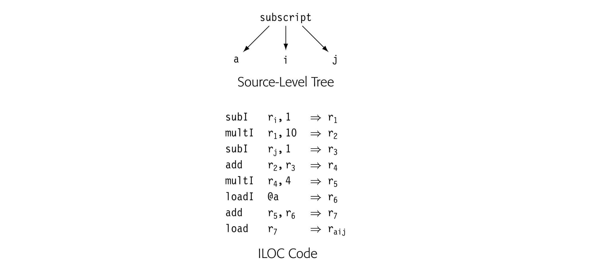
In the source-level tree, the compiler can easily recognize the computation as an array reference, whereas the ILOC code obscures that fact fairly well. In a compiler that tries to determine when two different references can touchthe same memory location, the source-level tree makes it easy to find and compare references. By contrast, the ILOC code makes those tasks hard. On the other hand, if the goal is to optimize the final code generated for the array access, the ILOC code lets the compiler optimize details that remain implicit in the source-level tree. For this purpose, a low-level IR may prove better.

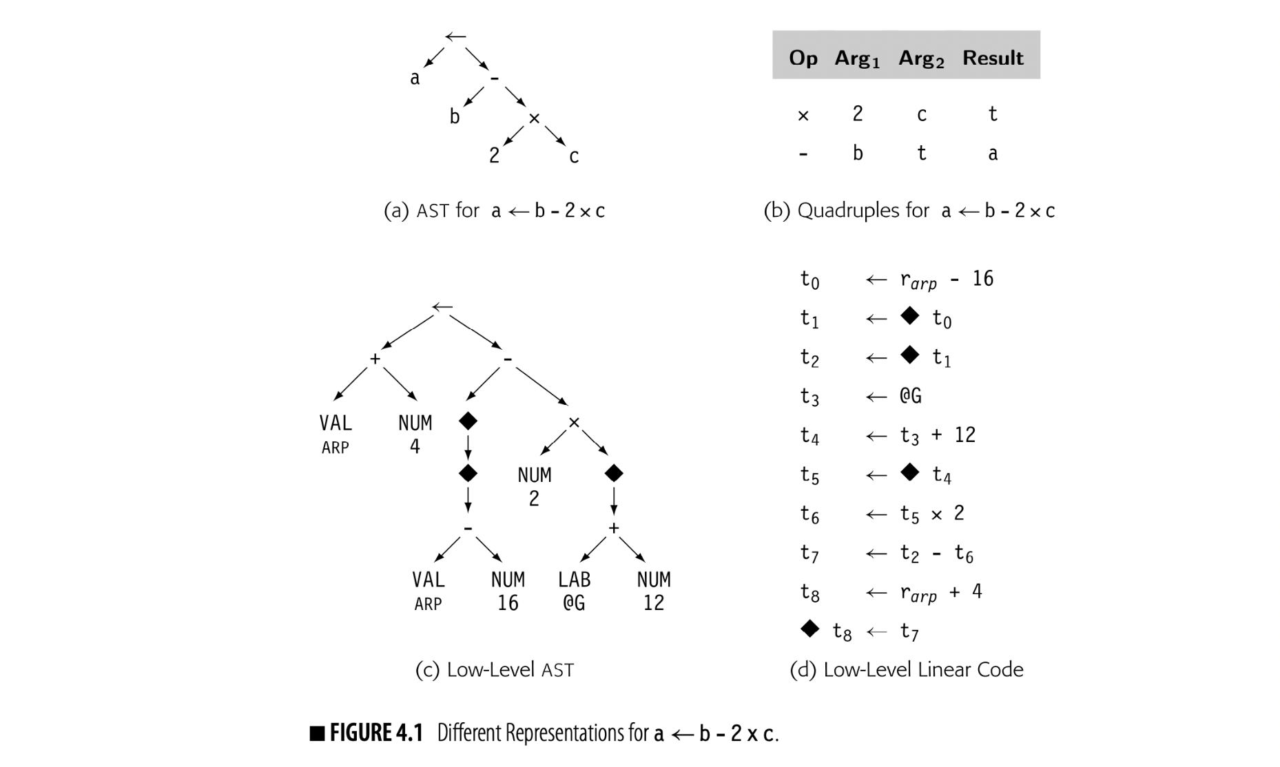
Level of abstraction is independent of structure. Fig. 4.1 shows four different representations for the statement a $\leftarrow$ b - 2 x c. Panels (a) and (c) show abstract syntax trees (ASTs) at both a near-source level and a near-machine level of abstraction. Panels (b) and (d) show corresponding linear representations.

The translation of $⧫$ in the low-level linear code depends on context. To the left of a $\leftarrow$ operator, it represents a store. To the right, it represents a load.

The low-level AST in panel (c) uses nodes that represent assembly-level concepts. A VAL node represents a value already in a register. A NUM node represents a known constant that can fit in an operation's immediate field. A LAB node represents an assembly-level label. The dereference operator, $⧫$ , treats the value as an address and represents a memory reference. This particular AST will reappear in Chapter 11.

Level of abstraction matters because the compiler can, in general, only optimize details that the IR exposes. Facts that are implicit in the IR are hard to change because the compiler treats implicit knowledge in uniform ways, which mitigates against context-specific customization. For example, to optimize the code for an array reference, the compiler must rewrite the IR for the reference. If the details of that reference are implicit, the compiler cannot change them.

Mode of Use

The third axis relates to the way that the compiler uses an IR.

A definitive IR is the primary representation for the code being compiled. The compiler does not refer back to the source code; instead, it analyzes, transforms, and translates one or more (successive) IR versions of the code. These IRs are definitive IRs.
A derivative IR is one that the compiler builds for a specific, temporary purpose. The derivative IR may augment the definitive IR, as with a dependence graph for instruction scheduling (see Chapter 12). The compiler may translate the code into and out of the derivative IR to enable a specific optimization.

In general, if an IR is transmitted from one pass to another, it should be considered definitive. If the IR is built within a pass for a specific purpose and then discarded, it is derivative.

Naming

The compiler writer must also select a name space for the IR. This decision will determine which values in the program are exposed to optimization. As it translates the source code, the compiler must choose names and storage locations for myriad distinct values.

Fig. 4.1 makes this concrete. In the ASTs, the names are implicit; the compiler can refer to any subtree in the AST by the node that roots the subtree. Thus, the tree in panel (c) names many values that cannot be named in panel (a), because of its lower level of abstraction. The same effect occurs in the linear codes. The code in panel (b) creates just two values that other operations can use while the code in panel (d) creates nine.

The naming scheme has a strong effect on how optimization can improve the code. In panel (d), t0 is the runtime address of b, t4 is the runtime address of c, and t8 is the runtime address of a. If nearby code references any of these locations, optimization should recognize the identical references and reuse the computed values (see Section 8.4.1). If the compiler reused the name t0 for another value, the computed address of b would be lost, because it could not be named.

REPRESENTING STRINGS

The scanner classifies words in the input program into a small set of categories. From a functional perspective, each word in the input stream becomes a pair ⟨ lexeme, category ⟩, where lexeme is the word’s text and category is its syntactic category. > For some categories, having both lexeme and category is redundant. The categories +, ×, and for have only one lexeme. For others, such as identifiers, numbers, and character strings, distinct words have distinct lexemes. For these categories, the compiler will need to represent and compare the lexemes. > >Character strings are one of the least efficient ways that the compiler can represent a name. The character string’s size is proportional to its length. To compare two strings takes, in general, time proportional to their length. A compiler can do better. >

The compiler should, instead, map the names used in the original code into a compact set of integers. This approach saves space; integers are denser than character strings. This approach saves time; comparisons for equality take $O (1)$ time.

To accomplish this mapping, the compiler writer can have the scanner create a hash table (see Appendix B.4) to hold all the distinct strings used in the input program. Then the compiler can use either the string’s index in this “string table” or a pointer to its record in the string table as a proxy for the string. Information derived from the string, such as the length of a string constant or the value and type of a numerical constant, can be computed once and referenced quickly through the table.

Using too few names can undermine optimization. Using too many can bloat some of the compile-time data structures and increase compile time without benefit. Section 4.6 delves into these issues.

Practical Considerations

As a practical matter, the costs of generating and manipulating an IR should concern the compiler writer, since they directly affect a compiler's speed. The data-space requirements of different IRs vary over a wide range. Since the compiler typically touches all of the space that it allocates, data space usually has a direct relationship to running time.

Last, and certainly not least, the compiler writer should consider the expressiveness of the IR--its ability to accommodate all the facts that the compiler needs to record. The IR for a procedure might include the code that defines it, the results of static analysis, profile data from previous executions, andmaps to let the debugger understand the code and its data. All of these facts should be expressed in a way that makes clear their relationship to specific points in the IR.

4.3 Graphical Irs

Many compilers use IRs that represent the underlying code as a graph. While all the graphical IRs consist of nodes and edges, they differ in their level of abstraction, in the relationship between the graph and the underlying code, and in the structure of the graph.

Parse trees, ASTs, and directed acyclic graphs (DAGs) are all graphs used to represent code. These tree-like IRs have a structure that corresponds to the syntax of the source code.

Parse Trees

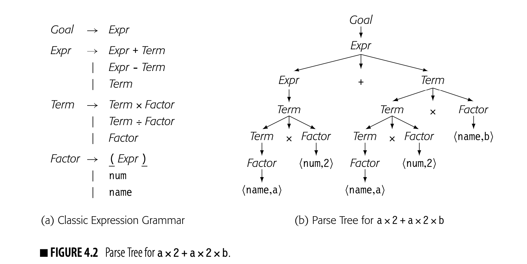
As we saw in Section 3.2, the parse tree is a graphical representation for the derivation, or parse, of the input program. Fig. 4.2 shows the classic expression grammar alongside a parse tree for $a \times 2 + a \times 2 \times b$ . The parse tree is large relative to the source text because it represents the complete derivation, with a node for each grammar symbol in the derivation. Since the compiler must allocate memory for each node and each edge, and it must traverse all those nodes and edges during compilation, it is worth considering ways to shrink this parse tree.

Minor transformations on the grammar, as described in Section 3.6.1, can eliminate some of the steps in the derivation and their corresponding parse-tree nodes. A more effective way to shrink the parse tree is to abstract away those nodes that serve no real purpose in the rest of the compiler. This approach leads to a simplified version of the parse tree, called an abstract syntax tree, discussed below.

Mode of Use: Parse trees are used primarily in discussions of parsing, and in attribute-grammar systems, where they are the definitive ir. In most other applications in which a source-level tree is needed, compiler writers tend to use one of the more concise alternatives, such as an ast or a dag.

Abstract Syntax Trees

Abstract syntax tree a contraction of the parse tree that omits nodes for most nonterminals

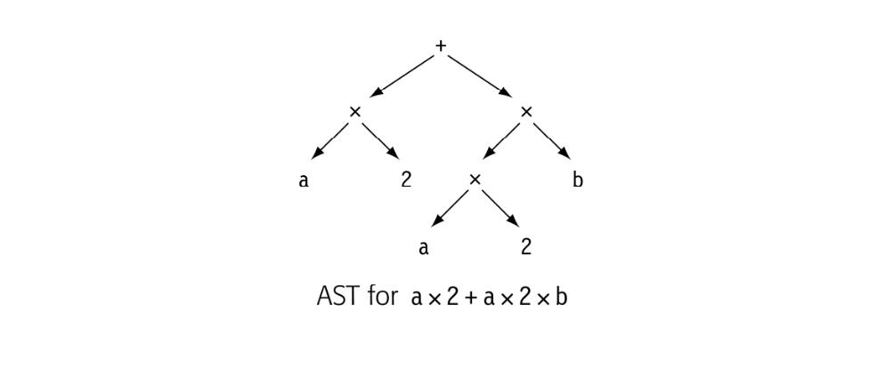
The abstract syntax tree (AST) retains the structure and meaning of the parse tree but eliminates extraneous nodes. It eliminates the nodes for non-terminal symbols that encode the details of the derivation. An ast for a x 2 + a x 2 $\times$ b is shown in the margin.

Mode of Use: ASTs have been used as the definitive ir in many practical compiler systems. The level of abstraction that those systems need varies widely.

Source-to-source systems, including syntax-directed editors, code-refactoring tools, and automatic parallelization systems, often use an ast with near-source abstractions. The structure of a near-source ast reflects the structure of the input program.
Compilers that generate assembly code may use an ast. These systems typically start with a near-source ast and systematically lower the level of abstraction until it is at or below the abstraction level of the target machine's isa. The structure of that final, low-level ast tends to reflect the flow of values between operations.

Ast-based systems usually use treewalks to traverse the ir. Many of the algorithms used in compilation have natural formulations as either a treewalk (see Section 11.4) or a depth-first search (see Section 8.5.1).

Some compilers build asts as derivative ir because conversion into and out of an ast is fast and because it may simplify other algorithms. In particular, optimizations that rearrange expressions benefit from building an ast as a derivative ir because the ast eliminates all of the explicit names for intermediate results. Other algorithms, such as tree-height balancing (Section 8.4.2) or tree-pattern matching (Section 11.4) have "natural" expressions as tree traversals.

CHOOSING THE RIGHT ABSTRACTION

Even with a source level tree, representation choices affect usability. For example, the Rn Programming Environment used the subtree shown in panel (a) below to represent a complex number in FORTRAN, which was written as (c1,c2). This choice worked well for the syntax-directed editor, in which the programmer was able to change c1 and c2 independently; the pair node corresponded to the parentheses and the comma. The pair format, however, proved problematic for the compiler. Each part of the compiler that dealt with constants needed special-case code for complex constants.

All other constants were represented with a single node that contained a pointer to the constant’s lexeme, as shown above in panel (b). Using a similar format for complex constants would have complicated the editor, but simplified the compiler. Taken over the entire system, the benefits would likely have outweighed the complications.

Directed Acyclic Graphs

Directed acyclic graph A DAG is an AST that represents each unique subtree once. DAGs are often called ASTs with sharing.

While an AST is more concise than a parse tree, it faithfully retains the structure of the original source code. For example, the AST for a x 2+ a x 2 x b contains two distinct copies of the expression a x 2. A directed acyclic graph (DAG) is a contraction of the AST that avoids this duplication. In a DAG, nodes can have multiple parents, and identical subtrees are reused. Such sharing makes the DAG more compact than the corresponding AST.

For expressions without assignment or function calls, textually identical expressions must produce identical values. The DAG for $a \times 2 + a \times 2 \times b$ , shown in the margin, reflects this fact by sharing a single copy of a x 2. If the value of a cannot change between the two uses of a, then the compiler should generate code to evaluate $a \times 2$ once and use the result twice. This strategy can reduce the cost of evaluation. The DAG explicitly encodes the redundancy among subexpressions. If the compiler represents such facts in the ir, it can avoid the costs of rediscovering them.

When building the DAG for this expression, the compiler must prove that a's value cannot change between uses. If the expression contains neither assignments nor calls to other procedures, the proof is easy. Since an assignment or a procedure call can change the value associated with a name, the DAG construction algorithm must invalidate subtrees when the values of their operands can change.

STORAGE EFFICIENCY AND GRAPHICAL REPRESENTATIONS

Many practical systems have used abstract syntax trees as their definitive IR. Many of these systems found that the AST was large relative to the size of the input text. In the $R^{n}$ Programming Environment built at Rice in the 1980s, AST size posed two problems: mid-1980s workstations had limited memory, and tree-l/O slowed down all of the $R^{n}$ tools.

$R^{n}$ AST nodes used 92 bytes. The IR averaged 11 nodes per sourcelanguage statement. Thus, the AST needed about 1,000 bytes per statement. On a 4MB workstation, this imposed a practical limit of about 1,000 lines of code in most of the environment's tools.

No single decision led to this problem. To simplify memory allocation, $R^{n}$ ASTs had only one kind of node. Thus, each node included all the fields needed by any node. (Roughly half the nodes were leaves, which need no pointers to children.) As the system grew, so did the nodes. New tools needed new fields.

Careful attention can combat this kind of node bloat. In $R^{n}$ , we built programs to analyze the contents of the AST and how it was used. We combined some fields and eliminated others. (In some cases, it was cheaper to recompute information than to write it and read it.) We used hash-linking to move rarely used fields out of the AST and into an ancillary table. (One bit in the node-type field indicated the presence of ancillary facts related to the node.) For disk I/O, we converted the AST to a linear form in a preorder treewalk, which made pointers implicit.

In $R^{n}$ , these changes reduced the size of ASTs in memory by about 75 percent. On disk, the files were about half the size of their memory representation. These changes let $R^{n}$ handle larger programs and made the tools noticeably more responsive.

Mode of Use: DAGs are used in real systems for two primary reasons. If memory constraints limit the size of programs that the compiler can process, using a DAG as the definitive IR can reduce the IR's memory footprint. Other systems use DAGs to expose redundancies. Here, the benefit lies in better compiled code. These latter systems tend to use the DAG as a derivative IR--build the DAG, transform the definitive IR to reflect the redundancies, and discard the DAG.

4.3.2 Graphs

While trees provide a natural representation for the grammatical structure that parsing discovers in the source code, their rigid structure makes them less useful for representing other properties of programs. To model these aspects of program behavior, compilers often use more general graphs as Its. The DAG introduced in the previous section is one example of a graph.

Control-Flow Graph

Basic block a maximal length sequence of branch-free code

The simplest unit of control flow is a basic block--a maximal length sequence of straight-line, or branch-free, code. The operations in a block always execute together, unless some operation raises an exception. A block begins with a labeled operation and ends with a branch, jump, or predicated operation. Control enters a basic block at its first operation. The operations execute in an order consistent with top-to-bottom order in the block. Control exits at the block's last operation.

Control-flow graph A CFG has a node for each basic block and an edge for each possible transfer of control.

A control-flow graph (CFG) models the flow of control between the basic blocks in a procedure. A CFG is a directed graph, $G = (N$ , $E)$ . Each node $n \in N$ corresponds to a basic block. Each edge $e = (n_{i}, n_{j}) \in E$ corresponds to a possible transfer of control from block $n_{i}$ to block $n_{j}$ .

If the compiler adds artificial entry and exit nodes, they may not correspond to actual basic blocks.

To simplify the discussion of program analysis in Chapters 8 and 9, we assume that each CFG has a unique entry node, $n_{0}$ , and a unique exit node, $n_{f}$ . If a procedure has multiple entries, the compiler can create a unique $n_{0}$ and add edges from $n_{0}$ to each actual entry point. Similarly, $n_{f}$ corresponds to the procedure's exit. Multiple exits are more common than multiple entries, but the compiler can easily add a unique $n_{f}$ and connect each of the actual exits to it.

The CFG provides a graphical representation of the possible runtime control-flow paths. It differs from syntax-oriented Its, such as an AST, which show grammatical structure. Consider the while loop shown below. Its CFG is shown in the center pane and its AST in the rightmost pane.

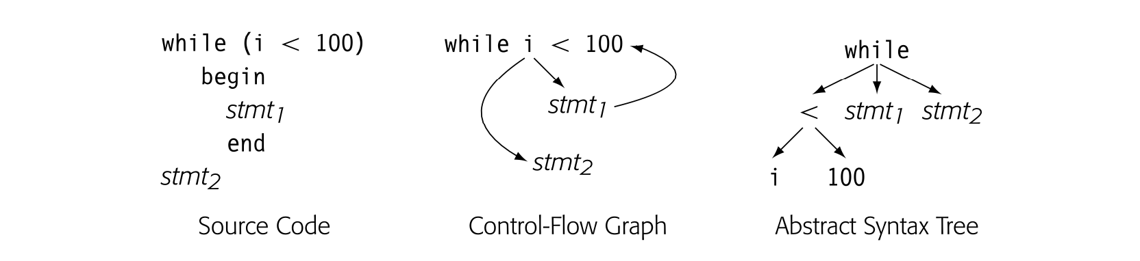
The CFG captures the essence of the loop: it is a control-flow construct. The cyclic edge runs from $stm t_{l}$ back to the test at the head of the loop. Bycontrast, the AST captures the syntax; it is acyclic but puts all the pieces in place to regenerate the source-code for the loop.

For an if-then-else construct both the CFG and the AST would be acyclic, as shown below. 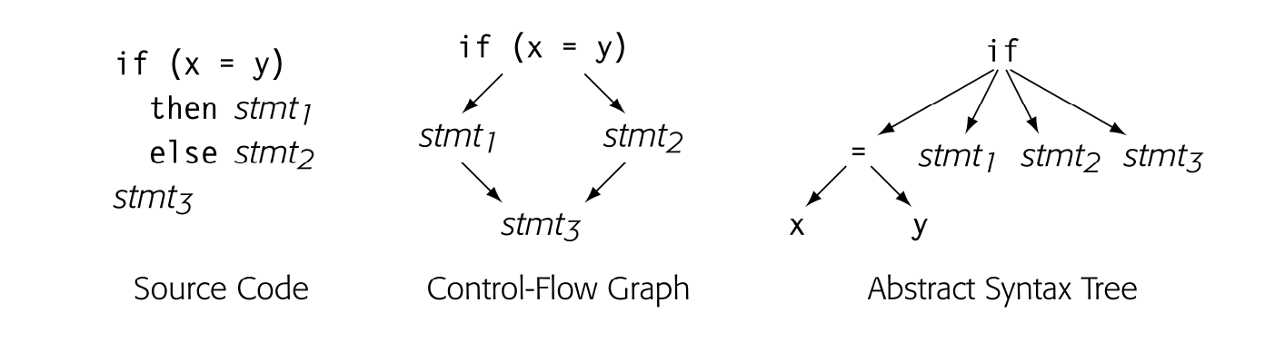Again, the CFG models the control flow; one of stmt1 or stmt2 executes, but not both of them. The AST again captures the syntax but provides little direct intuition about how the code actually executes. Any such connection is implicit, rather than explicit.

Mode of Use: Compilers typically use a CFG in conjunction with another IR, making the CFG a derivative IR. The CFG represents the relationships among blocks, while the operations inside a block are represented with an- other IR, such as an expression-level AST, a DAG, or one of the linear IRs. A compiler could treat such a hybrid IR as its definitive IR, but the complica- tions of keeping the multiple forms consistent makes this practice unusual.

Section 4.4.4 covers CFG construction.

Many parts of the compiler rely on a CFG, either explicitly or implicitly. Program analysis for optimization generally begins with control-flow anal- ysis and CFG construction (see Chapter 9). Instruction schedulers need a CFG to understand how the scheduled code for individual blocks flows to- gether (see Chapter 12). Register allocation relies on a CFG to understand how often each operation might execute and where to insert loads and stores for spilled values (see Chapter 13).

Block Length

Single-statement blocks a scheme where each block corresponds to a single source-level statement

Some authors recommend building CFGs around blocks that are shorter than a basic block. The most common alternative block is a single-statement block. Single-statement blocks can simplify algorithms for analysis and op- timization.

The tradeoff between a CFG built with single-statement blocks and one built with maximal-length blocks involves both space and time. A CFG built on single-statement blocks has more nodes and edges than one built on maximal-length blocks. Thus, the single-statement CFG will use more memory than the maximal-length CFG, other factors being equal. With more

nodes and edges, traversals take longer. More important, as the compiler annotates the CFG, the single-statement CFG has many more annotations than does the basic-block CFG. The time and space spent to build and use these annotations undoubtedly dwarfs the cost of CFG construction.

On the other hand, some optimizations benefit from single-statement blocks. For example, lazy code motion (see Section 10.3.1) only inserts code at block boundaries. Thus, single-statement blocks let lazy code motion optimize code placement at a finer granularity than would maximal-length blocks.

Dependence Graph

Data-dependence graph a graph that models the flow of values from definitions to uses in a code fragment

Compilers also use graphs to encode the flow of values from the point where a value is created, a definition, to any point where it is read, a use. A data-dependence graph embodies this relationship. Nodes in a data-dependence graph represent operations. Most operations contain both definitions and uses. An edge in a data-dependence graph connects two nodes, a definition in one and a use in the other. We draw dependence graphs with edges that run from the definition to the use; some authors draw these edges from the use to the definition.

Definition An operation that creates a value is said to define that value. Use An operation that references a value is called a use of that value.

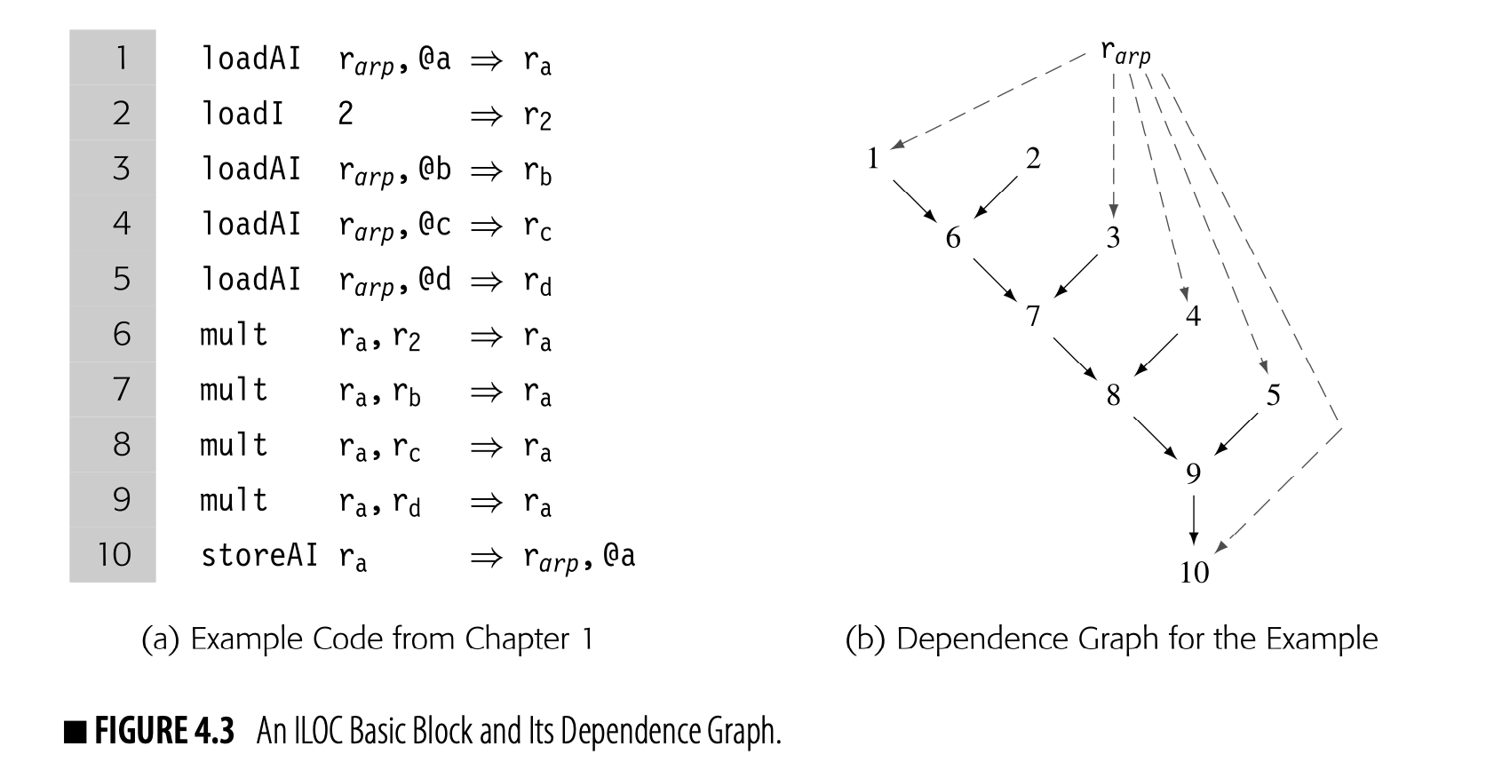
Fig. 4.3 shows ILOC code to compute a $a \leftarrow a \times 2 \times b \times c \times d$ , also shown in Fig. 4.4. Panel (a) contains the ILOC code. Panel (b) shows the corresponding data-dependence graph.

The dependence graph has a node for each operation in the block. Each edge shows the flow of a single value. For example, the edge from 3 to 7 reflects the definition of $r_{b}$ in statement 3 and its subsequent use in statement 7. The virtual register $r_{σ r p}$ contains an address that is at a fixed distance from the start of the local data area. Uses of $r_{σ r p}$ refer to its implicit definition at the start of the procedure; they are shown with dashed lines.

The edges in the graph represent real constraints on the sequencing of operations--a value cannot be used until it has been defined. The dependence graph edges impose a partial order on execution. For example, the graph requires that 1 and 2 precede 6. Nothing, however, requires that 1 or 2 precedes 3. Many execution sequences preserve the dependences shown in the graph, including $(1, 2, 3, 4, 5, 6, 7, 8, 9, 10)$ and $(2, 1, 6, 3, 7, 4, 8, 5, 9, 10)$ . The instruction scheduler exploits the freedom in this partial order, as does an "out-of-order" processor.

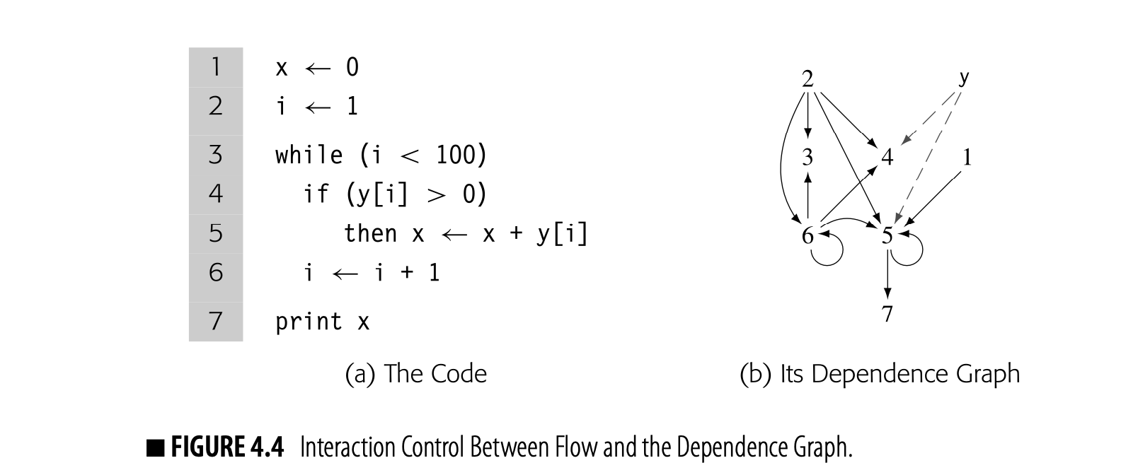
At a more abstract level, consider the code fragment shown in Fig. 4.4(a), which incorporates multiple basic blocks, along with both a while loop and an if-then construct. The compiler can construct a single dependence graph for the entire code fragment, as shown in panel (b).

References to $y [i]$ derive their values from a single node that represents all of the prior definitions of $y$ . Without sophisticated analysis of the subscript expressions, the compiler cannot differentiate between references to individual array elements.

This dependence graph is more complex than the previous example. Nodes 5 and 6 both depend on themselves; they use values that they may have defined in a previous iteration. Node 6, for example, can take the value of $i$ from either 2 (in the initial iteration) or from itself (in any subsequent iteration). Nodes 4 and 5 also have two distinct sources for the value of $i$ : nodes 2 and 6.

Mode of Use: Data-dependence graphs are typically built for a specific task and then discarded, making them a derivative IR. They play a central role in instruction scheduling (Chapter 12). They find application in a variety of optimizations, particularly transformations that reorder loops to expose parallelism and to improve memory behavior. In more sophisticated applications of the data-dependence graph, the compiler may perform ex- tensive analysis of array subscript values to determine when references to the same array can overlap.

Call Graph

Interprocedural Any technique that examines interactions across more than one procedure is called interprocedural.

To optimize code across procedure boundaries, some compilers perform interprocedural analysis and optimization. To represent calls between procedures, compilers build a call graph. A call graph has a node for each procedure and an edge for each distinct procedure call site. Thus, if the code calls $q$ from three textually distinct sites in $p$ , the call graph has three edges $(p, q)$ , one for each call site.

Intraprocedural Any technique that limits its attention to a single procedure is called intraprocedural.

Both software-engineering practice and language features complicate the construction of a call graph.

Call graph a graph that represents the calling relation- ships among the procedures in a program The call graph has a node for each proce- dure and an edge for each call site.

Separate compilation limits the compiler's ability to build a call graph because it limits the set of procedures that the compiler can see. Some compilers build partial call graphs for the procedures in a compilation unit and optimize that subset.
Procedure-valued parameters, both as actual parameters and as return values, create ambiguous calls that complicate call-graph construction. The compiler may perform an interprocedural analysis to limit the set of edges that such a call induces in the call graph, making call graph construction a process of iterative refinement. (This problem is analogous to the issue of ambiguous branches in CFG construction, as discussed in Section 4.4.4.)

Class hierarchy analysis a static analysis that builds a model of a program’s inheritance hierarchy

In object-oriented programs, inheritance can create ambiguous procedure calls that can only be resolved with additional type information. In some languages, class hierarchy analysis can disambiguate many of these calls; in others, that information cannot be known until runtime. Runtime resolution of ambiguous calls poses a serious problem for call graph construction; it also adds significant runtime overhead to the ambiguous calls.

Section 9.4 discusses some of the problems in call graph construction.

Mode of Use: Call graphs almost always appear as a derivative IR, built to support interprocedural analysis and optimization and then discarded. In fact, the best known interprocedural transformation, inline substitution (see Section 8.7.1), changes the call graph as it proceeds, rendering the old call graph inaccurate.

SECTION REVIEW

Graphical IRs present an abstract view of the code being compiled. The level of abstraction in a graphical IR, such as an AST, can vary from source level to below machine level. Graphical IRs can serve as definitive IRs or be built as special-purpose derivative IRs.

Because they are graphs, these IRs encode relationships that may be difficult to represent or manipulate in a linear IR. Graph traversals are an efficient way to move between logically connected points in the program; most linear IRs lack this kind of cross-operation connectivity.

REVIEW QUESTIONS

Given an input program, compare the expected size of the IR as a func- tion of the number of tokens returned by the scanner for (a) a parse tree, (b) an AST, and (c) a DAG. Assume that the nodes in all three IR forms are of a uniform and fixed size.

How does the number of edges in a dependence graph for a basic block grow as a function of the number of operations in the block?

4.4 Linear IRs

Linear IRs represent the program as an ordered series of operations. They are an alternative to the graphical IRs described in the previous section. An assembly-language program is a form of linear code. It consists of an ordered sequence of instructions. An instruction may contain more than one operation; if so, those operations execute in parallel. The linear IRs used in compilers often resemble the assembly code for an abstract machine.

The logic behind using a linear form is simple. The source code that serves as input to the compiler is a linear form, as is the target-machine code that it emits. Several early compilers used linear IRs; this was a natural notation for their authors, since they had previously programmed in assembly code.

Linear IRs impose a total order on the sequence of operations. In Fig. 4.3, contrast the ILOC code with the data-dependence graph. The ILOC code has an implicit total order; the dependence graph imposes a partial order that allows multiple execution orders.

If a linear IR is used as the definitive IR in a compiler, it must include a mechanism to encode transfers of control among points in the program. Control flow in a linear IR usually models the implementation of control flow on the target machine. Thus, linear codes usually include both jumps and conditional branches. Control flow demarcates the basic blocks in a linear IR; blocks end at branches, at jumps, or just before labeled operations.

Taken branch In most ISAs, conditional branches use only one label. Control flows either to the label, called the taken branch, or to the operation that follows the label, called the fall-through branch. The fall-through path is often faster than the taken path.

Branches in I L O C differ from those found in a typical assembly language. They explicitly specify a label for both the taken path and the fall-through path. This feature eliminates all fall-through transfers of control and makes it easier to find basic blocks, to reorder basic blocks, and to build a CFG.

Many kinds of linear IRs have been used in compilers.

■ One-address codes model the behavior of accumulator machines and stack machines. These codes expose the machine’s use of implicit names so that the compiler can tailor the code for it. The resulting IR can be quite compact.

Destructive operation an operation in which one of the operands is always redefined with the result These operations likely arose as a way to save space in the instruction format on 8- or 16-bit machines.

■ Two-address codes model a machine that has destructive operations. These codes fell into disuse as destructive operations and memory con- straints on IR size became less important; a three-address code can model destructive operations explicitly.

■ Three-address codes model a machine where most operations take two operands and produce a result. The rise of RISC architectures in the 1980s and 1990s made these codes popular again.

The rest of this section describes two linear IRs that are in common use: stack-machine code and three-address code. Stack-machine code offers a compact, storage-efficient representation. In applications where IR size mat- ters, such as a JAVA applet transmitted over a network before execution, stack-machine code makes sense. Three-address code models the instruction format of a modern RISC machine; it has distinct names for two operands and a result. You are already familiar with one three-address code: the ILOC used throughout this book.

4.4.1 Stack-Machine Code

Stack-machine code, a form of one-address code, assumes the presence of a stack of operands. It is easy to generate and to understand. Most operations read their operands from the stack and push their results onto the stack. For example, a subtract operator removes the top two stack elements and pushes their difference onto the stack.

The stack discipline creates a need for new operations: push copies a value from memory onto the stack, pop removes the top element of the stack and writes it to memory, and swap exchanges the top two stack elements. Stack-based processors have been built; the IR seems to have appeared as a modelfor those ISAs. Stack-machine code for the expression a - 2xb appears in the margin. Stack-machine code is compact. The stack creates an implicit name space and eliminates many names from the IR, which shrinks the IR. Using the stack, however, means that all results and arguments are transitory, unless the code explicitly moves them to memory.

Bytecode an IR designed specifically for its compact form; typically code for an abstract stack machine The name derives from its limited size; many operations, such as multiply, need only a single byte.

Mode of Use: Stack-machine code is typically used as a definitive ir--often as the IR to transmit code between systems and environments. Both SMALLtalk-80 and JAVA use bytecode, the ISA of a stack-based virtual machine, as the external, interpretable form for code. The bytecode either runs in an interpreter, such as the JAVA virtual machine, or is translated into native target-machine code before execution. This design creates a system with a compact form of the program for distribution and a simple scheme for porting the language to a new machine: implement an interpreter for the virtual machine.

4.4.2 Three-Address Code

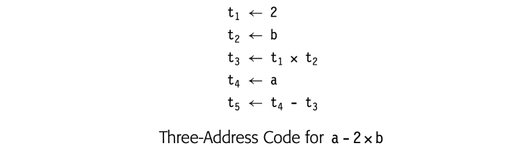In three-address code, most operations have the form i - j op k, with an operator (op), two operands (j and k), and one result (i). Some operators, such as an immediate load and a jump, use fewer arguments. Sometimes, an operation has more than three addresses, such as a floating-point multiply-add operation. Three-address code for a - 2xb appears in the margin. ILOC is a three-address code.

Three-address code is attractive for several reasons. First, it is reasonably compact. Most operations consist of four items: an operation code, or opcode, and three names. The opcode and the names are drawn from limited sets. Opcodes typically require one or two bytes. Names are typically represented by integers or table indices. Second, separate names for the operands and the result give the compiler freedom to specify and control the reuse of names and values; three-address code has no destructive operations. Three-address code introduces a new set of compiler-generated names--names that hold the results of the various operations. A carefully chosen name space can reveal new opportunities to improve the code. Finally, since many modern processors implement three-address operations, a three-address code models their properties well.

Level of Abstraction: Within three-address codes, the set of supported operators and the level of abstraction can vary widely. Often, a three-address IR will contain mostly low-level operations, such as jumps, branches, loads, and stores, alongside more complex operations that encapsulate control flow, such as max. Representing these complex operations directly simplifies analysis and optimization.

For example, consider an operation that copies a string of characters from one address, the source, to another, the destination. This operation appeared as the bcopy library routine in the 4.2 BSD UNIX distribution and as the mvcl instruction (move character long) in the IBM 370 ISA. On a machine that does not implement an operation similar to mvcl, it may take many operations to perform such a copy.

IBM’s PL.8 compiler, a pioneering RISC compiler, used this strategy.

Adding mvcl to the three-address code lets the compiler compactly represent this complex operation. The compiler can analyze, optimize, and move the operation without concern for its internal workings. If the hardware supports an mvcl-like operation, then code generation will map the IR construct directly to the hardware operation. If the hardware does not, then the compiler can translate mvcl into a sequence of lower-level IR operations or a call to a bcopy-like routine before final optimization and code generation.

Mode of Use: Compilers that use three-address codes typically deploy them as a definitive IR. Three-address code, with its explicit name space and its load-store memory model, is particularly well suited to optimization for register-to-register, load-store machines.

4.4.3 Representing Linear Codes

Many data structures have been used to implement linear IRs. The choices that a compiler writer makes affect the costs of various operations on IR code. Since a compiler spends most of its time manipulating the IR form of the code, these costs deserve some attention. While this discussion focuses on three-address codes, most of the points apply equally to stack-machine code (or any other linear form).

Three-address codes are often implemented as a set of quadruples. Each quadruple is represented with four fields: an operator, two operands (or sources), and a destination. To form blocks, the compiler needs a mechanism to connect individual quadruples. Compilers implement quadruples in a variety of ways.

Fig. 4.5 shows three schemes to represent three-address code for a-2xb (shown in the margin). The first scheme, in panel (a), uses an array of structures. The compiler might build such an array for each CFG node to hold the code for the corresponding block. In panel (b), a vector of pointers holds the block's quadruples. Panel (c) links the quadruples together into a list.

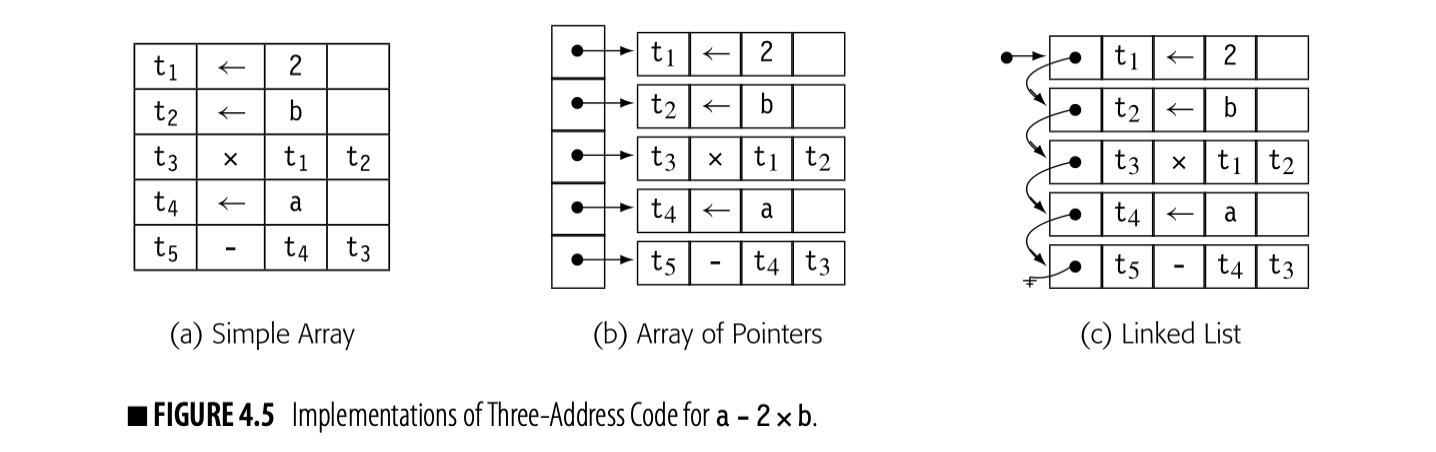
Consider the costs incurred to rearrange the code in this block. The first operation loads a constant into a register; on most machines this translatesdirectly into a load immediate operation. The second and fourth operations load values from memory, which on most machines might incur a multicycle delay unless the values are already in the primary cache. To hide some of the delay, the instruction scheduler might move the loads of b and a in front of the load immediate of 2.

In the array of structures, moving the load of b ahead of the immediate load requires saving the first operation to a temporary location, shuffling the second operation upward, and moving the immediate load into the second slot. The vector of pointers requires the same three-step approach, except that only the pointer values must be changed. The compiler can save the pointer to the immediate load, copy the pointer to the load of b into the first vector element, and rewrite the second vector element with the saved pointer. For the linked list, the operations are similar, except that the compiler must save enough state to let it traverse the list.

Now, consider what happens in the front end when it generates the initial round of ir. With the array of structures and the vector of pointers, the compiler must select a size for the array--in effect, the number of quadruples that it expects in a block. As it generates the quadruples, it fills in the data structure. If the compiler allocated too much space, that space is wasted. If it allocated too little, the compiler must allocate space for a larger array or vector, copy the contents into this new place, and free the original space. The linked list avoids these problems. Expanding the list just requires allocating a new quadruple and setting the appropriate pointer in the list.

A multipass compiler may use different implementations to represent the ir at different points in the compilation process. In the front end, where the focus is on generating the ir, a linked list might both simplify the implementation and reduce the overall cost. In an instruction scheduler, with its focus on rearranging the operations, the array of pointers might make more sense. A common interface can hide the underlying implementation differences.

INTERMEDIATE REPRESENTATIONS IN ACTUAL USE

In practice, compilers use a variety of IRs. Legendary FORTRAN compilers of yore, such as IBM’s FORTRAN H compilers, used a combination of quadruples and control-flow graphs to represent the code for optimization. Since FORTRAN H was written in FORTRAN, it held the IR in an array.

For years, GCC relied on a very low-level IR, called register transfer language (RTL). GCC has since moved to a series of IRs. The parsers initially produce a language-specific, near-source tree. The compiler then lowers that tree to a second IR, GIMPLE, which includes a language-independent tree-like structure for control-flow constructs and three-address code for expressions and assignments. Much of GCC’s optimizer uses GIMPLE; for example, GCC builds static single-assignment form (SSA) on top of GIMPLE. Ultimately, GCC translates GIMPLE into RTL for final optimization and code generation.

The LLVM compiler uses a single low-level IR; in fact, the name LLVM stands for “low-level virtual machine.” LLVM’s IR is a linear three-address code. The IR is fully typed and has explicit support for array and structure addresses. It provides support for vector or SIMD data and operations. Scalar values are maintained in SSA form until the code reaches the compiler’s back end. In LLVM environments that use GCC front ends, LLVM IR is produced by a pass that performs GIMPLE-to-LLVM translation.

The Open64 compiler, an open-source compiler for the IA-64 architecture, used a family of five related IRs, called WHIRL. The parser produced a near-source-level WHIRL. Subsequent phases of the compiler introduced more detail to the WHIRL code, lowering the level of abstraction toward the actual machine code. This scheme let the compiler tailor the level of abstraction to the various optimizations that it applied to IR.

Notice that some information is missing from Fig. 4.5. For example, no labels are shown because labels are a property of the block rather than any individual quadruple. Storing a list of labels with the CFG node for the block saves space in each quadruple; it also makes explicit the property that labels occur only at the start of a block. With labels attached to a block, the compiler can ignore them when reordering operations inside the block, avoiding one more complication.

4.4.4 Building the CFG from Linear Code

Compilers often must convert between different its, often different styles of its. One routine conversion is to build a CFG from a linear IR such as ILOC. The essential features of a CFG are that it identifies the beginning and end of each basic block and connects the resulting blocks with edges thatdescribe the possible transfers of control among blocks. Often, the compiler must build a CFG from a simple, linear IR that represents a procedure.

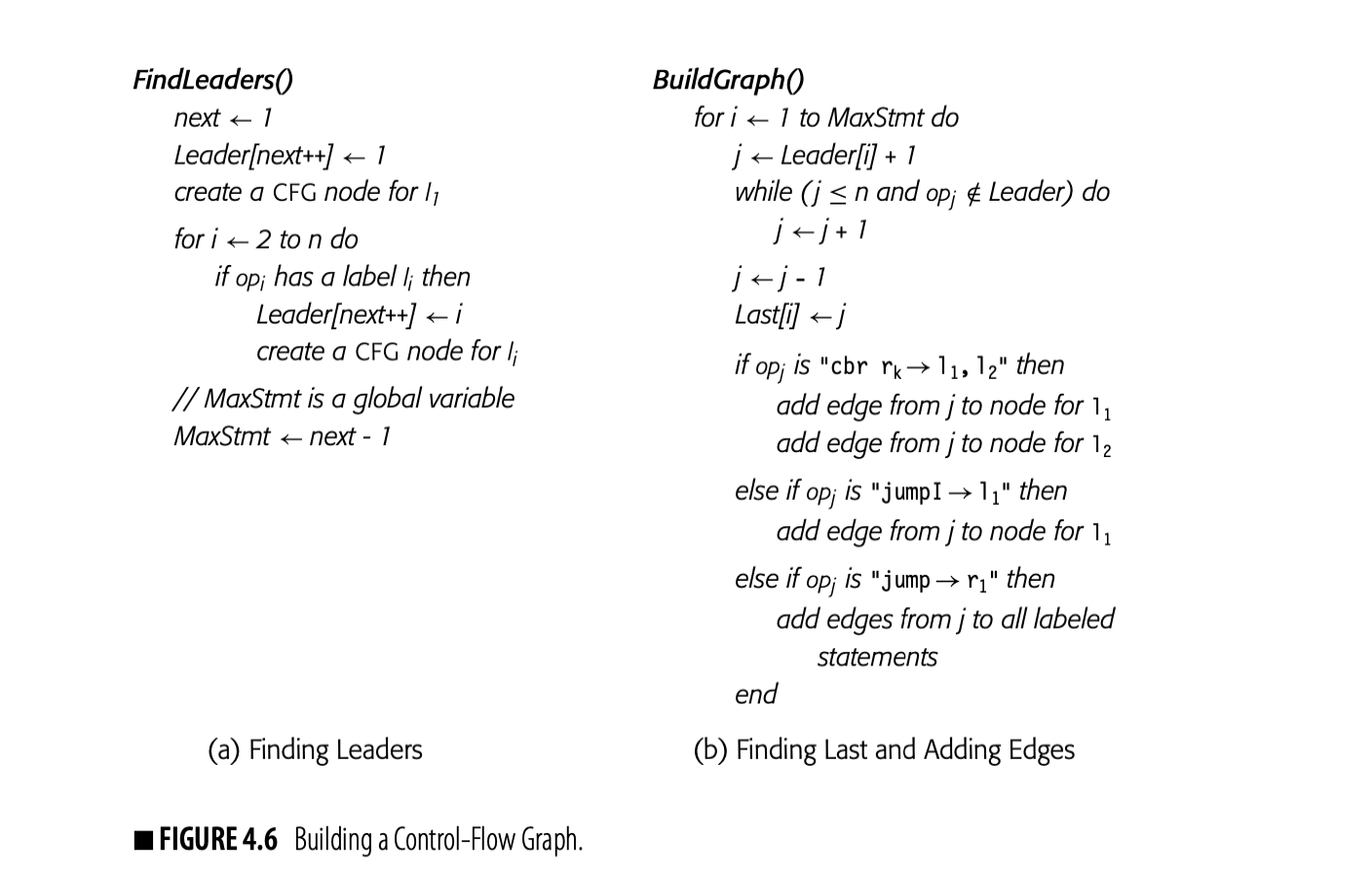
As a first step, the compiler must find the start and the end of each basic block in the linear IR. We will call the initial operation of a block a leader. An operation is a leader if it is the first operation in the procedure, or if it has a label that is, potentially, the target of some branch. The compiler can identify leaders in a single pass over the IR, shown in Fig. 4.6(a). FindLeaders iterates over the operations in the code, in order, finds the labeled statements, and records them as leaders.

Ambiguous jump a branch or jump whose target is not known at compile time (e.g., a jump to an address in a register) In ILOC, jump is ambiguous while jumpI is not.

If the linear IR contains labels that are not used as branch targets, then treating labels as leaders may unnecessarily split blocks. The algorithm could track which labels are jump targets. However, ambiguous jumps may force it to treat all labeled statements as leaders.

CFG construction with fall-through branches is left as an exercise for the reader (see Exercise 4).

The second pass, shown in panel (b), finds every block-ending operation. It assumes the ILOC model where every block, except the final block, ends with a branch or a jump and branches specify labels for both the taken and not-taken paths. This assumption simplifies the handling of blocks and allows the compiler's optimizer or back end to choose which path will be the "fall through" case of a branch. (For the moment, assume branches have no delay slots.)

To find the end of each block, the algorithm iterates through the blocks, in order of their appearance in the Leader array. It walks forward through the IR until it finds the leader of the next block. The operation immediately before that leader ends the current block. The algorithm records that operation's index in $L os t [j]$ , so that the pair \text{\langle Leader[j], Lost[j] \rangle} describes block $i$ . It adds edges to the CFG as needed.

For a variety of reasons, the CFG should have a unique entry node $n_{0}$ and a unique exit node $n_{f}$ . If the underlying code does not have this shape, a simple postpass over the graph can create $n_{0}$ and $n_{f}$ .

Complications in CFG Construction

Features of the IR, the target machine, and the source language can complicate CFG construction.

Pseudooperation an operation that manipulates the internal state of the assembler or compiler, but does not translate into an executable operation

Ambiguous jumps may force the compiler to add edges that are not feasible at runtime. The compiler writer can improve this situation by recording the potential targets of ambiguous jumps in the IR. IOC includes the tb1 pseudooperation to specify possible targets of an ambiguous jump (see Appendix A). Anytime the compiler generates a jump, it should follow the jump with one or more tb1 operations that record the possible targets. The hints reduce spurious edges during CFG construction.

PC-relative branch A transfer of control that specifies an offset, either positive or negative, from its own memory address.

If a tool builds a CFG from target-machine code, features of the target ISA can complicate the process. The algorithm in Fig. 6.4.6 assumes that all leaders, except the first, are labeled. If the target machine has fall-through branches, the algorithm must be extended to recognize unlabeled statements that receive control on a fall-through path. PC-relative branches cause a similar set of complications.

Branch delay slots introduce complications. The compiler must group any operation in a delay slot into the block that preceded the branch or jump. If that operation has a label, it is a member of multiple blocks. To disambiguate such an operation, the compiler can place an unlabeled copy of the operation in the delay slot and use the labeled operation to start the new block.

If a branch or jump can occur in a branch delay slot, the CFG builder must walk forward from the leader to find the block-ending branch--the first branch it encounters. Branches in the delay slot of a block-ending branch can be pending on entry to the target block. In effect, they can split the target block into multiple blocks and create both new blocks and new edges. This feature adds serious complications to CFG construction.

Some languages allow jumps to labels outside the current procedure. In the procedure that contains the jump, the jump target can be modeled with a new block. In the procedure that contains the target, however, the labeled block can pose a problem. The compiler must know that the label is the target of a nonlocal jump; otherwise, analysis passes may produce misleading results. For this reason, languages such as PASCAL or ALGOL restricted nonlocal jumps to visible labels in outer lexical scopes. C requires the use of the functions setjmp and longjmp to expose these transfers.

SECTION REVIEW

Linear IRs represent the code being compiled as an ordered sequence of operations. Linear IRs vary in their level of abstraction; the source code for a program in a text file is a linear form, as is the assembly code for that same program. Linear IRs lend themselves to compact, human-readable representations.

Two widely used linear IRs are bytecodes, generally implemented as a one-address code with implicit names on many operations, and three-address code, similar to ILOC.

REVIEW QUESTIONS

Consider the expression $a \times 2 + a \times 2 \times b$ . Translate it into stack-machine code and into three address code. Compare and contrast the total num- ber of operations and operands in each form. How do they compare to the tree in Fig. 4.2(b)?

Sketch the modifications that must be made to the algorithm in Fig. 4.6 to account for ambiguous jumps and branches. If all jumps and branches are labeled with a construct similar to ILOC’s tbl, does that simplify your algorithm?

4.5 Symbol Tables

Symbol table

A collection of one or more data structures that hold information about names and values Most compilers maintain symbol tables as persistent ancillary data structures used in conjunction with the IR that represents the executable code.

During parsing the compiler discovers the names and properties of many distinct entities, including named values, such as variables, arrays, records, structures, strings, and objects; class definitions; constants; labels in the code; and compiler-generated temporary values (see the digression on page 192).

For each name actually used in the program, the compiler needs a variety of information before it can generate code to manipulate that entity. The specific information will vary with the kind of entity. For a simple scalar variable the compiler might need a data type, size, and storage location. For

a function it might need the type and size of each parameter, the type and size of the return value, and the relocatable assembly-language label of the function’s entry point.

Thus, the compiler typically creates one or more repositories to store de- scriptive information, along with an efficient way to locate the information associated with a given name. Efficiency is critical because the compiler will consult these repositories many times.

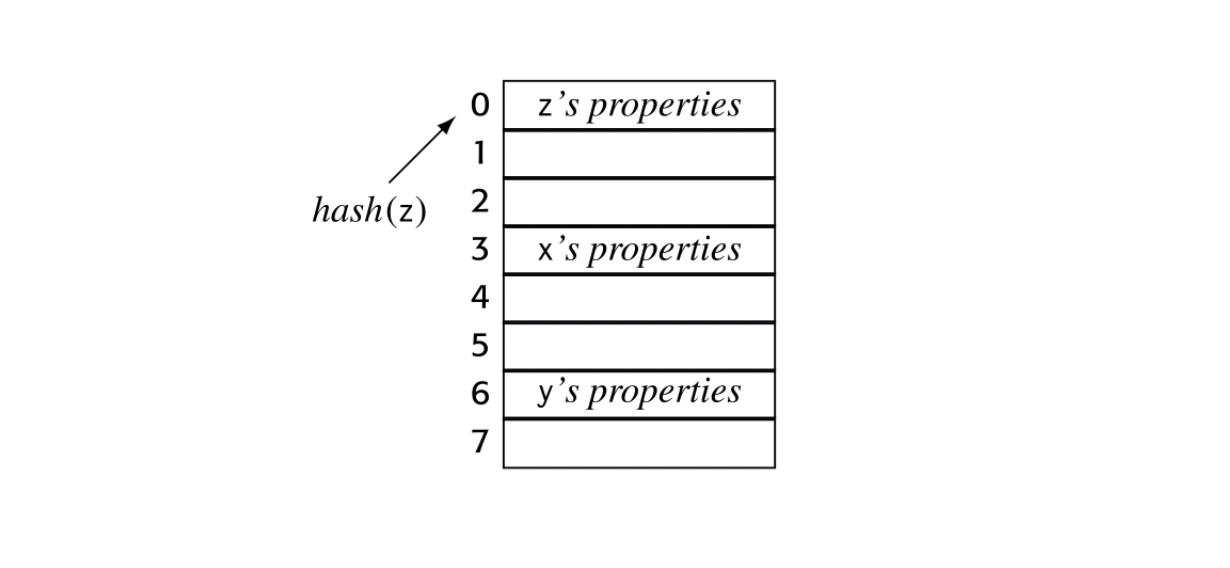
The compiler typically keeps a set of tables, often referred to as symbol tables. Conceptually, a symbol table has two principal components: a map from textual name to an index in a repository and a repository where that index leads to the name’s properties. An abstract view of such a table is shown in the margin.

Constant pool a statically initialized data area set aside for constant values

A compiler may use multiple tables to represent different kinds of informa- tion about different kinds of values. For names, it will need a symbol table that maps each name to its properties, declared or implicit. For aggregates, such as records, arrays, and objects, the compiler will need a structure table that records the entity’s layout: its constituent members or fields, their prop- erties, and their relative location within the structure. For literal constants, such as numbers, characters, and strings, the compiler will need to lay out a data area to hold these values, often called a constant pool. It will need a map from each literal constant to both its type and its offset in the pool.

4.5.1 Name Resolution

The primary purpose of a symbol table is to resolve names. If the compiler finds a reference to name $n$ at some point $p$ in a program, it needs a mechanism that maps $n$ back to its declaration in the naming environment that holds at $p$ . The map from name to declaration and properties must be well defined; otherwise, a program might have multiple meanings. Thus, programming languages introduce rules that specify where a given declaration of a name is both valid and visible.

Scope the region of a program where a given name can be accessed

In general, a scope is a contiguous set of statements in which a name is declared, visible, and accessible. The limits of a scope are marked by specific symbols in the language. Typically, a new procedure defines a new scope that covers its entire definition. C and C++ demarcate blocks with curly braces. Each block defines a new scope.

REPRESENTING REFERENCES IN THE IR

In the implementation of an IR, the compiler writer must decide how to represent a reference to a source language name. The compiler could simply record the lexeme; that decision, however, will require a symbol-table lookup each time that the compiler uses the reference.

The best alternative may be to store a handle to the relevant symbol table reference. That handle could be an absolute pointer to the table entry; it might be a pointer to the table and an offset within the table. Such a handle will allow direct access to the symbol table information; it should also enable inexpensive equality tests.

In most languages, scopes can nest. A declaration for $x$ in an inner scope obscures any definitions of $x$ in surrounding scopes. Nesting creates a hierarchy of name spaces. These hierarchies play a critical role in softwareengineering; they allow the programmer to choose local names without concern for their use elsewhere in the program.

The two most common name-space hierarchies are created by lexical scope rules and inheritance rules. The compiler must build tables to model each of these hierarchies.

Lexical Scopes

A lexical-scoping environment uses properly nested regions of code as scopes. A name $n$ declared in scope $s$ is visible inside $s$ . It is visible inside any scope nested in $s$ , with the caveat that a new declaration of $n$ obscures any declaration of $n$ from an outer scope.

Global scope an outer scope for names visible in the entire program

At a point $p$ in the code, a reference to $n$ maps to the first declaration of $n$ found by traversing the scopes from the scope containing the reference all the way out to the global scope. Lexically scoped languages differ greatly in the depth of nesting that they allow and the set of scopes that they provide. (Sections 5.4.1, 6.3.1, and 6.4.3 discuss lexical scopes in greater depth.)

Inheritance Hierarchies

Superclass and Subclass In a language with inheritance, if class x inherits members and properties from class y, we say that x is a subclass of y and y is the superclass of x. The terminology used to specify inheri- tance varies across languages. In JAVA, a subclass extends its superclass. In C++, a subclass is derived from its superclass.

Object-oriented languages (OOLs) introduce another set of scopes: the inheritance hierarchy. OOLs create a data-centric naming scheme for objects; objects have data and code members that are accessed relative to the object rather than relative to the current procedure.

In an OOL, explicitly declared subclass and superclass relationships define the inheritance hierarchy--a naming regime similar to the lexical hierarchy and orthogonal to it. Conceptually, subclasses nest within superclasses, just as inner scopes nest within outer scopes in a lexical hierarchy. The compiler builds tables to model subclass and superclass relationships, as well.

Hierarchical Tables

The compiler can link together tables, built for individual scopes, to represent the naming hierarchies in any specific input program. A typical program in an Algol-like language (all) might have a single linked set of tables to represent the lexically nested scopes. In an OOL, that lexical hierarchy would be accompanied by another linked set of tables to represent the inheritance hierarchy.

When the compiler encounters a reference in the code, it first decides whether the name refers to a variable (either global or local to some method) or an object member. That determination is usually a matter of syntax; languages differentiate between variable references and object references. For a variable reference, it begins in the table for the current scope and searches upward until it finds the reference. For an object member, it determines the object's class and begins a search through the inheritance hierarchy.

In a method $m$ , declared in some class $c$ , the search environment might look as follows. We refer to this scheme as the "sheaf of tables."

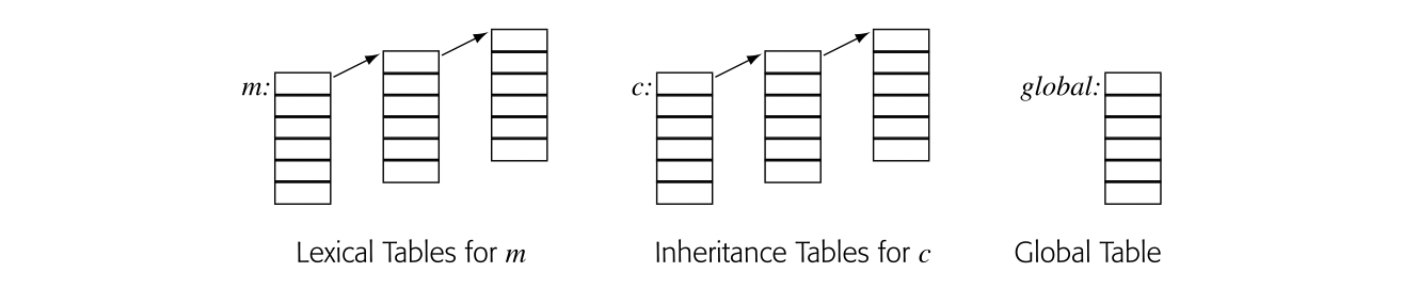The lookup begins in the table for the appropriate scope and works its way up the chain of tables until it either finds the name or exhausts the chain. Chaining tables together in this fashion creates a flexible and powerful tool to model the complex scoping environments of a modern programming language.

The compiler writer can model complex scope hierarchies--both lexical hierarchies and inheritance hierarchies--with multiple tables linked together in a way that reflects the language-designated search order. For example, nested classes in JAVA give rise to a lexical hierarchy within the inheritance hierarchy. The link order may vary between languages, but the underlying technology need not change.

In a modern environment, the compiler will likely retain each of these tables for later use, either in the compiler or in related tools such as performance monitors or debuggers. The sheaf-of-tables approach can create compact, separable tables suitable for preservation.

Other Scopes

Other language features create nested scopes. For example, records, structures, and objects all act as independent scopes. Each creates a new name space and has a set of visibility rules. The compiler may or may not choose to implement these scopes with a full-blown sheaf in a hash table; nonetheless each is a distinct scope and can be modeled with a new sheaf in the appropriate table. The constant pool might also be treated as a separate scope.

4.5.2 Table Implementation

As we have seen, a compiler will contain multiple distinct tables, ranging from symbol tables and inheritance tables through structure layout tables and constant tables. For each table, the compiler writer must choose an appropriate implementation strategy: both a mapping function and a repository. While the choices are, for the most part, independent, the compiler writer may want to use the same basic strategies across multiple tables so that they can share implementations.

Implementing the Mapping

The mapping from a textual name to an index can be implemented in myriad ways, each with their own advantages and disadvantages.

Linear List

A linear list is simple to construct, to expand, and to search. The primary disadvantage of a linear list is that searching the list takes \mathsf{O}\big{(}n\big{)} time per lookup, where $n$ is the number of items in the list. Still, for a small procedure, a linear list might make sense.

Tree

A tree structure has the advantages of a list, including simple and efficient expansion. It also has the potential to significantly reduce the time required per lookup. Assuming that the tree is roughly balanced--that is, the subtrees at each level are approximately the same size--then the expected case lookup time should approach \mathsf{O}\big{(}\log_{2}n\big{)} per item, where $n$ is the number of items in the tree.

Balanced trees use more complex insertion and deletion protocols to maintain roughly equal-sized subtrees. The literature contains many effective and efficient techniques for building balanced trees.

Unbalanced trees have simpler insertion and deletion protocols but provide no guarantees on the relative sizes of sibling subtrees. An unbalanced tree can devolve into linear search when presented with an adversarial input.

Hash Map

The compiler can use a numerical computation, called a hash, to produce an integer from a string. A well-designed hash function,, distributes those integers so that few strings produce the same hash value. To build a hash table, the programmer uses the hash value of a string, modulo the table size, as an index into a table.

Hash collision When two strings map to the same table index, we say that they collide. For hash function h(x) and table size s, if $h (x) mod s = h (y) mod s,$ then x and y will collide.

Handling collisions is a key issue in hash table design, as discussed in Appendix B.4. If the set of keys produces no collisions, then insertion and lookup in a hash table should take $O (1)$ . If the set of keys all map to the same table index, then insertion and lookup might devolve to $O (∣ k eys ∣)$ time per lookup. To avoid this problem, the compiler writer should use a well-designed hash function, as found in a good algorithms textbook.

Static Map

As an alternative to hashing, the compiler can precompute a collision-free static map from keys to indices. Multiset discrimination solves this problem (see the digression on page 190).

For small sets of keys, an approach that treats the keys as a set of acyclic regular expressions and incrementally builds a to recognize that set can lead to a fast implementation (see Section 2.6.2). Once the transition-table size exceeds the size of the level-one data cache, this approach slows down considerably.

Implementing the Repository

The implementation of the repository storage for the information associated with a given name can be orthogonal to the lookup mechanism. Different tables may need distinct and different structures to accommodate the kinds of information that the compiler needs. Nonetheless, these repositories should have some common properties (see also Appendix B.4).

Block contiguous These allocators use two protocols: a ma- jor allocation obtains space for multiple records while a minor one returns a single record. Minor allocations use a fast method; they amortize the major allocation cost over many records.

Record storage should be either contiguous or block-contiguous to improve locality, decrease allocation costs, and simplify reading and writing the tables to external media.
Each repository should contain enough information to rebuild the lookup structure, in order to accommodate graceful table expansion, and to facilitate restoring the structures from external media.
The repository should support changes to the search path. For example, as the parser moves in and out of different scopes, the search path should change to reflect the current situation.

From a management perspective, the repository must be expandable in order to handle large programs efficiently without wasting space on small ones. Its index scheme should be independent of the mapping scheme so that the map can be expanded independently of the repository; ideally, the map will be sparse and the repository dense.

SECTION REVIEW

Compilers build ancillary data structures to augment the information stored in the compiler’s definitive IR. The most visible of these structures is a set of symbol tables that map a name in the source text or the IR into the set of properties associated with that name.

This section explored several issues in the design of these ancillary tables. It showed how linking tables together in explicit search paths can model both lexical scope rules and inheritance rules. It discussed tradeoffs in the implementation of both the mapping mechanism and the repository for these tables.

REVIEW QUESTIONS

Using the “sheaf-of-tables” scheme, what is the complexity of inserting a new name into the table at the current scope? What is the complexity of looking up a name in the set of tables? How deep are the lexical and inheritance hierarchies in programs that you write?

When the compiler initializes a scope, it likely needs an initial symbol table size. How might the parser estimate that initial symbol table size? How might later passes of the compiler estimate it?

4.6 Name Spaces

Most discussions of name spaces focus on the source program's name space: lexical scopes and inheritance rules. Of equal importance, from the perspective of the quality of compiled code, is the name space created in the compiler's IR. A specific naming discipline can either expose opportunities for optimization or obscure them. The choices that the compiler makes with regard to names determine, to a large extent, which computations can be analyzed and optimized.

AN ALTERNATIVE TO HASHING

Symbol tables are often implemented with hash maps, due to the expected efficiency of hashing. If the compiler writer is worried about the unlikely but possible worst-case behavior of hashing, multiset discrimination provides an interesting alternative. It avoids the possibility of worst-case behavior by constructing the index offline, in the scanner.

To use multiset discrimination, the compiler first scans the entire program and builds a ⟨name,pos⟩ tuple for each instance of an identifier, where name is the identifier’s lexeme and pos is its ordinal position in the list of classified words, or tokens. It enters all the tuples into a large set.

Next, the compiler sorts the set lexicographically. In effect, this creates a set of subsets, one per identifier. Each subset holds the tuples for all the occurrences of its identifier. Since each tuple refers to a specific token, through its position value, the compiler can use the sorted set to modify the token stream. The compiler makes a linear scan over the set, processing each subset. It allocates a symbol-table index for each unique identifier, then rewrites the tokens to include that index. The parser can read symbol-table indices directly from the tokens. If the compiler needs a textual lookup function, the resulting table is ordered alphabetically for a binary search.

This technique adds some cost to compilation. It makes an extra pass over the token stream, along with a lexicographic sort. In return, it avoids any possibility of worst-case behavior from hashing and it makes the initial size of the symbol table obvious before parsing begins. This technique can replace a hash table in almost any application in which an offline solution will work.

The IR name space is intimately related to the memory model used in translation. The compiler may assume that all values are kept in memory, except when they are actively used in a computation. The compiler may assume that values are kept in registers whenever possible. If the compiler uses stack-machine code as its IR, it will keep these active values on the stack. These different assumptions radically affect the set of values that can be named, analyzed, and optimized.

This section focuses on issues in name space design; it also introduces one important example: static single assignment form. The next section explores the issues that arise in choosing a memory model.

4.6.1 Name Spaces in the IR

When compiler writers design an IR, they should also design a naming discipline for the compiler to follow. The choice of a name space interacts with the choice of an IR; some IRs allow broad latitude in naming, while others make most names implicit in the representation.

Implicit Versus Explicit Names

Tree-like IRs use implicit names for some values. Consider an AST for $a - 2 \times b$ , shown in the margin. It has nodes for each of a, 2, b, $2 \times b$ , and $a - 2 \times b$ . The interior nodes, those for $2 \times b$ and $a - 2 \times b$ , lack explicit names that the compiler can manipulate. 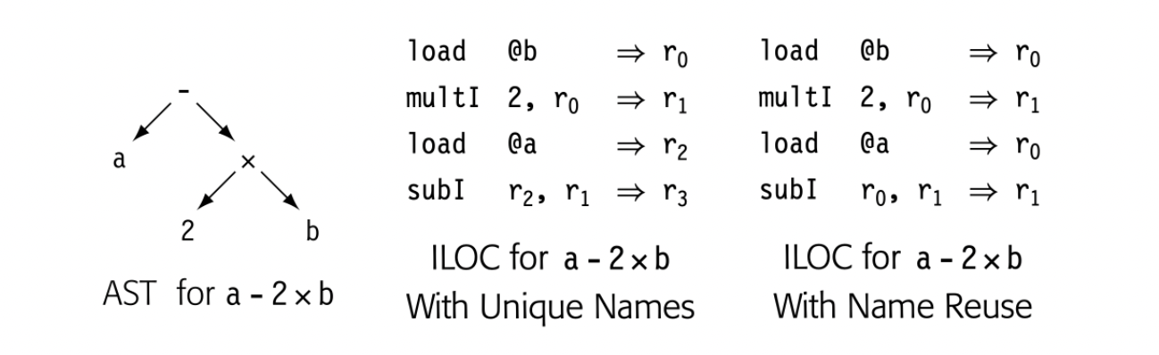By contrast, three-address code uses only explicit names, which gives the compiler control over the naming discipline. It can assign explicit names to any or all of the values computed in the code. Consider, for example, the ILOC code for a-2xb, shown in the margin. The upper version introduces a unique name for every unknown value and expression--register names $r_{0}$ through $r_{3}$ . After execution, each of those values survives in its own register. The lower version uses a different naming discipline intended to conserve names. After it executes, the two quantities that survive are a in $r_{0}$ and a-2xb in $r_{1}$ .

The example makes it appear that graphical IRs use implicit names and linear IRs use explicit names. It is not that simple. Stack-machine code relies on an implicit stack data structure, which leads to implicit names for many values. A CFG has explicit names for each of the nodes so that they can be connected to the corresponding code fragments. Even an AST can be rewritten to include explicit names; for any expression or subexpression that the compiler wants to name, it can insert an assignment and subsequent use for a compiler-generated name.

Variables Versus Values

In the source program, the set of accessible names is determined by the source language rules and the details of the program. Declared named variables are visible; intermediate subexpressions are not. In the statement: a, b, and c can each be used in subsequent statements. The values of 2*b, c/3, and cos(c/3) cannot.

Virtual name A compiler-generated name is often called a virtual name, in the same sense as virtual memory or a virtual register.

In the IR form of the code, the compiler writer must decide which values to expose via consistent, explicit names. The compiler can use as many names as necessary; compiler writers sometimes refer to these generated names as virtual names. The compiler might translate the statement so that the code evaluates each of these three expressions into its own unique name. Alternatively, by reusing names, it could eliminate any chance for reuse.

The impact of naming

In the late 1980s, we experimented with naming schemes in a FORTRAN 77 compiler. The first version generated a new name for each computation; it simply bumped a counter to get a new name. This approach produced large name spaces; for example, 985 names for a 210-line implementation of the singular value decomposition (SVD). Objectively, this name space seemed large. It caused speed and space problems in the register allocator, where name space size determines the size of many data structures. (Today, we have better data structures, and much faster machines with more memory).

The second version used an allocate/free protocol to manage names. The front end allocated temporary names on demand and freed them when the immediate uses were finished. This scheme shrank the name space; SVD used roughly 60 names. Allocation was faster; for example, the time to compute LwCount sets for SVD decreased by 60 percent (see Section 8.6.1).

Unfortunately, reuse of names obscured the flow of values and degraded the quality of optimization. The decline in code quality overshadowed any compile-time benefits.

Further experimentation led to a short set of rules that yielded strong optimization while mitigating growth in the name space.

Each textual expression received a unique name, found by hashing. Thus, each occurrence of an expression, for example, $r_{1} + r_{2L}$ targeted the same register.

In (op) $r_{i}, r_{j} \Rightarrow r_{k} k$ was chosen so that $i, j < k$ .

Register copy operations, $r_{i} \Rightarrow r_{j}$ , were allowed to have $i > j$ only if $r_{j}$ corresponded to a declared scalar variable. Registers for variables were only defined by copy operations. Expressions were evaluated into their "natural" register and then were moved into the register for the variable.

Each store operation, $r_{i} \Rightarrow MEM (r_{j})$ , was followed by a copy from $r_{i}$ into the variable's named register. (Rule 1 ensures that loads from that location always target the same register. Rule 4 ensures that the virtual register and memory location contain the same value.)

With this name space, the compiler used about 90 names for SVD. It exposed all of the optimizations found with the first name-space scheme. The compiler used these rules until we adopted the SSA name space.

This decision has a direct effect on what the compiler can do in subsequent optimization.

The compiler writer enforces these decisions by codifying them in the translation rules that generate the ir. These decisions have a widespread effect on the efficiency of both the compiler and the code that it generates.

The temptation, of course, is to provide a unique name for each subexpression, so as to maximize the opportunities presented to the optimizer. However, not all subexpressions are of interest. A value that is only live in a single block does not need a name that persists through the entire procedure. Exposing such a value to procedure-wide analysis and optimization is unlikely to change the code.

The converse is true, as well. Any value that is live in multiple blocks or is computed in multiple blocks may merit an explicit, persistent name. Expressions that are computed in multiple blocks, on multiple paths, are prime targets for a number of classical global optimizations. Providing a single consistent name across multiple definitions and uses can expose an expression to analysis and transformations that improve the compiled code (see Chapters 8-10).

Finally, the choice of a naming discipline also interacts with decisions about the level of abstraction in the IR. Consider again the two representations of an array reference, a[i,j], shown in the margin. The source-level AST, along with the symbol table, contains all of the essential information needed to analyze or translate the reference. (The symbol table will contain a's type, data area, and offset in that data area along with the number of dimensions and their upper and lower bounds.) The corresponding ILOC code exposes more details of the address calculations and provides explicit names for each subexpression in that calculation.

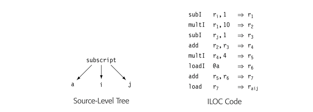
These two representations expose and name different quantities. The AST explicitly exposes the fact that the calculation computes the address for a[i,j], but shows no details of that calculation. The ILOC code exposes the fact that the address computation involves seven distinct subexpressions, any one of which might occur elsewhere. The question of which IR is better depends entirely on how the compiler writer intends to use the information.

4.6.2 Static Single-Assignment Form

SSA form an IR that has a value-based name system, created by renaming and use of pseudoop- erations called $ϕ$ -functions SSA encodes both control and value flow. It is used widely in optimization (see Section 9.3).

Static single-assignment form (SSA) is an IR and a naming discipline that many modern compilers use to encode information about both the flow of control and the flow of values in the program. In SSA form, each name corresponds to one definition point in the code. The term static single assignment refers to this fact. As a corollary, each use of a name in an operation encodes information about where the value originated; the textual name refers to a specific definition point.

$ϕ$ -function
A $ϕ$ -function takes several names and merges them, defining a new name.

A program is in SSA form when it meets two constraints: (1) each definition has a distinct name; and (2) each use refers to a single definition. To transform an IR program to SSA form, the compiler inserts $ϕ$ -functions at points where different control-flow paths merge and it then renames variables so that the single-assignment property holds.

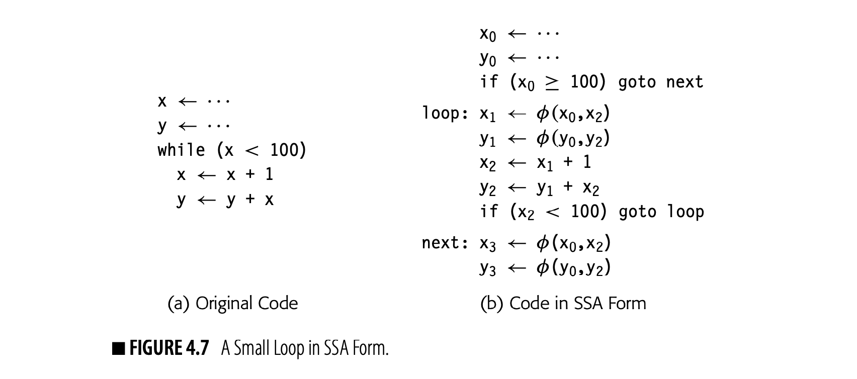
The code shape for the loop is discussed in Section 7.5.2.

To clarify the impact of these rules, consider the small loop shown in Fig. 4.7(a). Panel (b) shows the same code in SSA form. Variable names include subscripts to create a distinct name for each definition. $ϕ$ -functions have been inserted at points where multiple distinct values can reach the start of a block. Finally, the while construct has been rewritten at a lower level of abstraction to expose the fact that the initial test refers to x0 while the end-of-loop test refers to x2.

The $ϕ$ -function has an unusual semantics. It acts as a copy operation that selects, as its argument, the value that corresponds to the edge along which control entered the block. Thus, when control flows into the loop from the block above the loop, the $ϕ$ -functions at the top of the loop body copy the values of x0 and y0 into x1 and y1, respectively. When control flows into the loop from the test at the loop's bottom, the $ϕ$ -functions select their other arguments, x2 and y2.

The definition of SSA form prevents two $ϕ$ -functions from defining the same SSA name.

The execution semantics of $ϕ$ -functions are different than other operations. On entry to a block, all its $ϕ$ -functions read the value of their appropriate argument, in parallel. Next, they all define their target SSA names, in parallel. Defining their behavior in this way allows the algorithms that manipulate SSA form to ignore the ordering of $ϕ$ -functions at the top of a block--an important simplification. It does, however, complicate the process of translating SSA form back into executable code, as discussed in Section 9.3.5.

Lifetime For a value a, its lifetime spans from its first definition to its last use.

SSA form was intended for analysis and optimization. The placement of φ-functions in SSA form encodes information about the creation and use of individual values. The single-assignment property of the name space al- lows the compiler to ignore many issues related to the lifetimes of values;

BUILDING SSA Static single-assignment form is the only IR we describe that does not have an obvious construction algorithm. Section 9.3 presents one construction algorithm in detail. However, a sketch of the construction process will clarify some of the issues. Assume that the input program is already in ILOC form. To convert it to an equivalent linear form of SSA, the compiler must first insert $ϕ$ -functions and then rename the ILOC virtual registers.

The simplest way to insert $ϕ$ -functions is to find each block that has multiple CFG predecessors and add a $ϕ$ -function for each ILOC virtual register at the start of that block. This process inserts many unneeded $ϕ$ -functions; most of the complexity in the full algorithm focuses on eliminating those extraneous $ϕ$ -functions.

To rename the ILOC virtual registers, the compiler can process the blocks, in a depth-first order. For each virtual register, it keeps a counter. When the compiler encounters a definition of $r_{i}$ , it increments the counter for $r_{i}$ , say to k, and rewrites the definition with the name $r_{i_{k}}$ . As the compiler traverses the block, it rewrites each use of $r_{i}$ with $r_{i_{k}}$ until it encounters another definition of $r_{i}$ . (That definition bumps the counter to $k + 1$ .) At the end of a block, the compiler looks down each control-flow edge and rewrites the appropriate $ϕ$ -function parameter for $r_{i}$ in each block that has multiple predecessors.

After renaming, the code conforms to the two rules of SSA form. Each definition creates a unique name. Each use refers to a single definition. Several better SSA construction algorithms exist; they insert fewer \phi-functions than this simple approach.

for example, because names are not redefined, the value of a name is available along any path that proceeds from that operation. These two properties simplify and improve many optimizations.

The example exposes some oddities of SSA form that bear explanation. Consider the $ϕ$ -function that defines $x_{1}$ . Its first argument, $x_{0}$ , is defined in the block that precedes the loop. Its second argument, $x_{2}$ , is defined later in the block labeled loop. Thus, when the $ϕ$ first executes, one of its arguments is undefined. In many programming-language contexts, this would cause problems. Since the $ϕ$ -function reads only one argument, and that argument corresponds to the most recently taken edge in the CFG, it can never read the undefined value.

A $ϕ$ -function takes an arbitrary number of operands. To fit SSA form into a three-address ir, the compiler writer must include mechanisms to accommodate longer operand lists and to associate those operands with specific 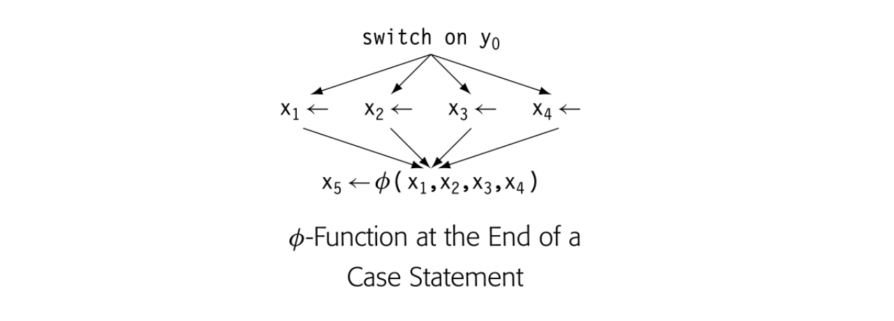The $ϕ$ -function for $x_{5}$ must have an argument for each case. The number of arguments it needs is bounded only by the number of paths that enter the block. Thus, an operation to represent that $ϕ$ -function in a linear IR will need an arbitrary number of arguments. It does not fit directly into the fixed-arity, three-address scheme.

In a simple array representation for three-address code, the compiler writer will need a side data structure to hold $ϕ$ -function arguments. In the other two schemes for implementing three-address code shown in Fig. 4.5, the compiler can insert tuples of varying size. For example, the tuples for load and load immediate might have space for just two names, while the tuple for a $ϕ$ -operation could be large enough to accommodate all its operands, plus an operand count.

SECTION REVIEW The compiler must generate internal names for all the values computed in a program. Those names may be explicit or implicit. The rules used to generate names directly affect the compiler’s ability to analyze and optimize the IR. Careful use of names can encode and expose facts for later use in optimization. Proliferation of names enlarges data structures and slows compilation.

The SSA name space encodes properties that can aid in analysis and optimization; for example, it lets optimizations avoid the need to reason about redefinitions of names (see Section 8.4.1). This additional precision in naming can both simplify algorithms and improve the optimizer’s results.

REVIEW QUESTIONS

The ILOC code shown in the margin on page 193 uses as many virtual register names as practical-assuming that $r_{i}$ and $r_{j}$ cannot be renamed because they represent variables in the program. Construct an equivalent code that uses as few virtual names as possible.

Convert the code shown in the margin to SSA form, following the explanation on page 195 . Does each $ϕ$ -functions that you inserted serve a purpose?

4.7 Placement of Values in Memory

Almost every ir has an underlying storage map. The compiler must assign a storage location to each value that the compiled code computes or uses. That location might be in a register or in memory. It might be a specific location: a physical register or (base address.offset) pair. It might be a symbolic location: a virtual register or a symbolic label. The location's lifetime must match the lifetime of the value; that is, it must be available and dedicated to the value from the time the value is created until the time of its last use.

This section begins with a discussion of memory models--the implicit rules used to assign values to data areas. The later subsections provide more detail on data area assignment and layout.

4.7.1 Memory Models

Before the compiler can translate the source program into its IR form, the compiler must understand, for each value computed in the code, where that value will reside. The compiler need not enumerate all the values and their locations, but it must have a mechanism to make those decisions consistently and incrementally as translation proceeds. Typically, compiler writers make a set of decisions and then apply them throughout translation. Together, these rules form a memory model for the compiled code.

Memory models help define the underlying model of computation: where does an operation find its arguments? They play a critical role in determining which problems the compiler must solve and how much space and time it will take to solve them.

Active value A value is active in the immediate neigh- borhood where it is used or defined.

Three memory models are common: a memory-to-memory model, a register-to-register model, and a stack model. These models share many characteristics; they differ in where they store values that are active in the current computation.

Memory-to-Memory Model Values have their primary home in memory. Either the IR supports memory-to-memory operations, or the code moves active values into registers and inactive values back to memory.

Register-to-Register Model Whenever possible, values are kept in a virtual register; some local, scalar values have their only home in a virtual register. Global values have their homes in memory (see Section 4.7.2).

Stack Model Values have their primary home in memory. The compiler moves active values onto and off of the stack with explicit operations (e.g., push and pop). Stack-based IRs and ISAs often include operations to reorder the stack (e.g., swap).

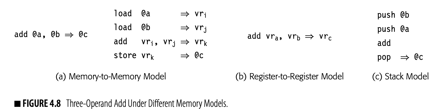
Unambiguous value A value that can be accessed with just one name is unambiguous.

Ambiguous value Any value that can be accessed by multiple names is ambiguous.

Fig. 4.8 shows the same add operation under each of these models. Panel (a) shows the operation under two different assumptions. The left column assumes that the add takes memory operands, shown as symbolic labels. The right column assumes that the add is a register-to-register operation, with values resident in memory. The choice between these two designs probably depends on the target machine's ISA. Panel (b) shows the same add in a register-to-register model. It assumes that a, b, and c are all unambiguous scalar values that reside in virtual registers: v $r_{a}$ , v $r_{b}$ , and v $r_{c}$ , respectively. Panel (c) shows the operation under a stack model; it assumes that the variable's home locations are in memory and named by symbolic labels.

These distinct memory models have a strong impact on the shape of the IR code and on the priorities for the optimizer and back end.

In a memory-to-memory model, the unoptimized form of the code may use just a few registers. That situation places a premium on optimizations that promote values into unused registers for nontrivial parts of their lifetimes. In the back end, register allocation focuses more on mapping names than on reducing demand for physical registers.
In a register-to-register model, the unoptimized code may use many more virtual registers than the target machine supplies. That situation encourages optimizations that do not significantly increase demand for registers. In the back end, register allocation is required for correctness and is one of the key determiners of runtime performance.

The JAVA HotSpot server compiler trans- lated JAVA bytecode to a graphical IR for optimization and code generation.

In a stack model, the structure of the target machine becomes critical. If the ISA has stack operations, as does the JAVA virtual machine, then optimization focuses on improving the stack computation. If the ISA is a Cisc or RISC processor, then the compiler will likely translate the stack-machine code into some other form for code generation.

In the end, the choice of memory model has a strong influence on the design of the compiler's optimizer and back end.

The hierarchy of memory operations in ILOC 9X

Under any memory model, the compiler writer should look for ways to encode more facts about values into the IR. In the 1990s, we built a research compiler that used an IR named ILOC 9x. The IR featured a hierarchy of memory operations that allowed the compiler to encode knowledge about values kept in memory. At the bottom of the hierarchy, the compiler had little or no knowledge about the value; at the top of the hierarchy, it knew the actual value. These operations are as follows:

Operation	Meaning
Immediate load Nonvarying load	Loads a known constant value into a register. Loads a value that does not change at runtime. The compiler does not know the value but can prove that the program does not change it.
Scalar load & store	Operate on a scalar value, not an array element, a structure element, or a pointer-based value.
Generic load & store	Operate on a value that may vary and may be non- scalar. It is the general-case operation.

With this hierarchy, the front end encoded knowledge about the target value directly into the ILOC 9x code. Other passes could rewrite operations from a more general to a more restricted form as they discovered new facts. For example, if the compiler discovered that a load always produced a known constant value, it replaced the generic or scalar load with an immediate load.

Optimizations capitalized on the facts encoded in this way. For example, a comparison between the result of a nonvarying load and a constant must itself be invariant—a fact that might be difficult or impossible to prove with a generic load operation.

4.7.2 Keeping Values in Registers

Spill

A register allocator spills a value by storing it to a designated location in memory. It may later restore the value to a register.

With a register-to-register memory model, the compiler tries to assign as many values as possible to virtual registers. This approach relies heavily on the register allocator to map virtual registers in the IR to physical registers in the final code, and to spill to memory any virtual register that it cannot keep in a physical register.

The compiler cannot keep an ambiguous value in a register across an assignment. With an unambiguous value $x$ , the compiler knows precisely where $x$ 's value changes: at assignments to $x$ . Thus, the compiler can safely generate code that keeps $x$ in a register.

With an ambiguous value $x$ , however, an assignment to some other ambiguous value $y$ might change $x$ 's value. If the compiler tries to hold $x$ in a register across an assignment to $y$ , the register may not be updated with the new value. To make matters worse, in a given procedure, $x$ and $y$ might refer to the same storage location in some invocations and not in others. This situation makes it difficult for the compiler to generate correct code that keeps $x$ in a register. Relegating $x$ to memory lets the addressing hardware resolve which assignments should change $x$ and which should not.

If a call passes a global name to a call-by- reference parameter, the callee can access the value with either its global name or the formal parameter name. The same effect occurs when a call passes a name x in two different call-by-reference parameter slots.

In practice, compilers decide which values they consider unambiguous, and relegate all ambiguous values to storage in memory--one of the data areas or the heap--rather than in a register. Ambiguity can arise in multiple ways. Values stored in pointer-based variables are often ambiguous. Call-by-reference parameters can be ambiguous. Many compilers treat array-element values as ambiguous because the compiler cannot tell if two references, such as A[i,j] and A[m,n] can ever refer to the same element.

Typically, compilers focus on proving that a given value is unambiguous. The analysis might be cursory and local. For example, in C, any local variable whose address is never taken is unambiguous. More complex analyses build sets of possible names for each pointer variable; any variable whose set has just one element is unambiguous. Analysis cannot resolve all ambiguities; the unprovable cases are treated as if they were proven to be ambiguous.

Language features can affect the compiler's ability to analyze ambiguity. For example, ANSI C includes two keywords that directly communicate information about ambiguity. The restrict keyword informs the compiler that a pointer is unambiguous. It is often used when a procedure passes an address directly at a call site. The volatile keyword lets the programmer declare that the contents of a variable may change arbitrarily and without notice. It is used for hardware device registers and for variables that might be modified by interrupt service routines or other threads of control in an application.

4.7.3 Assigning Values to Data Areas

Data area A region in memory set aside to hold data values. Each data area is associated with some specific scope. Examples include local data areas for pro- cedures and global data areas.

Just as the compiler must choose a name for each value in the program, so, too, must it decide where those values will reside at runtime. While the memory model determines where values live while they are active, each of the memory models discussed in Section 4.7.1 consigns some values to memory when they are not active. The compiler must decide, for each such value, where it should reside during its lifetime.

Most temporary values will live in the space reserved for active values--either registers or memory locations in the local data area--as determined by both the memory model and the availability of space. For variables that are declared in the source program, the compiler assigns each one a permanent home, based on its individual properties: its lifetime, its visibility, and its declaring scope.

Lifetime A value's lifetime refers to the period of time during which its value can be defined or referenced. Outside of a value's lifetime, it is undefined.

Region of Visibility A value is visible if it can be named--that is, the code can read or write the value. Its region of visibility is, simply, the code in which it is visible.

Declaring Scope A variable's lifetime and visibility depend on the scope that declares it. For example, a file static variable in C has a lifetime of the entire execution; it is only visible inside the file that declares it.

Programming languages have rules that determine lifetime, visibility, and scope for each name.

To simplify memory management, most compilers create a set of data areas associated with various program scopes. For memory resident variables, the combination of lifetime, visibility, and declaring scope determines which data area will hold the variable's value.

From a storage layout perspective, the compiler will categorize lifetimes into one of three categories.

Automatic A name whose lifetime matches a single activation of the scope that declares it is an automatic variable.

Automatic An automatic variable's lifetime matches one activation of its scope (a procedure or block). The value is defined and used inside the scope and its value ceases to exist on exit from the scope. A local variable is, typically, automatic by default.

We call these variables "automatic" because their allocation and deallocation can be handled as part of entry and exit for the corresponding scope. At runtime, each invocation of a procedure has its own local data area where automatic variables can be stored.

Static A name that retains its value across mul- tiple activations of its scope is a static variable.

Static A static variable's lifetime might span multiple activations of its declaring scope. If it is assigned a value, that value persists after control exists the scope where the assignment occurred.

The compiler can allocate such variables once, before execution; they are, in effect, always present. Static variables are stored in a preallocated data area associated with the declaring scope. The compiler may combine the static data areas for multiple scopes.

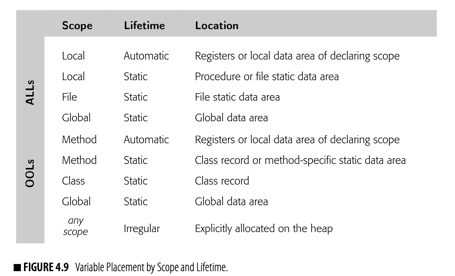
Constant values are a special case; they are static values that can be initialized with an assembly-level directive. The compiler typically creates a separate data area for them, often called a constant pool.

Irregular An entity whose lifetime depends on ex- plicit allocation and either explicit or implicit deallocation is an irregular entity.

Irregular An irregular variable has a lifetime that is not tied to any single scope. It is, typically, allocated explicitly; it may be freed either explicitly or implicitly. Examples include objects in JAVA and strings created with malloc in C.

Variables with irregular lifetimes are, in general, allocated space on the runtime heap (see Section 5.6.1).

The compiler can categorize each value by its lifetime and scope. This classification suggests a specific data area for the value's storage. Fig. 4.9 shows a typical scheme that a compiler might use to place variables into registers and data areas.

Given a mapping from values to data areas, the compiler must assign each memory-resident value a location. It iterates over the data areas and, within a data area, over the values for that data area. It assigns each value a specific offset from the start of the data area. Algorithms for this assignment are discussed in Section 5.6.3.

For values that might be kept in registers, the compiler assigns them a virtual register name. The actual assignment of virtual registers to hardware registers is left to the register allocator.

SECTION REVIEW The compiler must determine, for each value that the program computes, where that value will reside at runtime. The compiler determines those locations based on the programming language, on the memory model adopted by the compiler, on lifetime information for the values, and on the compiler writer’s knowledge of the target machine’s system architecture. The compiler systematically assigns each value to a register or a data area and assigns offsets within data areas to individual values. Decisions about the placement of values can affect the performance of compiled code. Storage layout can change the locality behavior of the program. Storage assignment decisions can encode subtle knowledge about properties of the underlying code, such as the ambiguity of values.

REVIEW QUESTIONS

Consider the function fib shown in the margin. Write down the ILOC that a compiler’s front end might generate for this code using a register-to-register model and using a memory-to-memory model. How does the code for the two models compare?

Write the pseudocode for an algorithm that takes a list of variables assigned to some data area and assigns them offsets. Explain what in- formation the compiler needs for each variable.

4.8 Summary and Perspective

The choice of an IR has a major impact on the design, implementation, speed, and effectiveness of a compiler. None of the intermediate forms de- scribed in this chapter are, definitively, the right answer for all compilers or all tasks in a given compiler. The compiler writer must consider the overall goals of a compiler project when selecting an IR, designing its im- plementation, and adding ancillary data structures such as symbol and label tables.

Contemporary compiler systems use all manner of IRs, ranging from parse trees and abstract syntax trees (often used in source-to-source systems) through lower-than-machine-level linear codes (used, for example, in GCC). Many compilers use multiple IRs—building a second or third one to per- form a particular analysis or transformation, then modifying the original, and definitive, one to reflect the result.

Chapter Notes

The literature on IRs and experience with them is sparse. Nonetheless, IRs have a major impact on both the structure and behavior of a compiler. The classic IR forms, such as syntax trees, ASTs, DAGs, quadruples, triples, and one-address code have been described in textbooks since the 1970s [8, 36,157,181]. New IR forms like SSA[56,120,279] are described in the literature on analysis and optimization. The original JAVA HotSpot Server compiler used a form of program dependence graph as its definitive IR[92]. Muchnick discusses IRs in detail and highlights the use of multiple levels of IR in a single compiler [279].

The observation that multiple passes over the code can lead to more efficient code dates back to Floyd [160]; this fundamental observation creates the need for IR and justifies the added expense of the multipass compiler. This insight applies in many contexts within a compiler.

The idea of using a hash function to recognize textually identical operations dates back to Ershov [150]. Its specific application in Lisp systems seems to appear in the early 1970s [135,174]; by 1980, it was common enough that McCarthy mentions it without citation [267].

Cai and Paige introduced multiset discrimination as an alternative to hashing [71]. Their intent was to create an efficient lookup mechanism with guaranteed constant time behavior. Closure-free regular expressions, described in Section 2.6.2, can achieve a similar effect. The work on shrinking the size of $R^{n}$ 's AST was done by David Schwartz and Scott Warren.

Exercises

Section 4.3

Both a parse tree and an abstract syntax tree retain information about the form of the source program.
What is the relationship between the size of the parse tree and the size of the input program?
What is the relationship between the size of the abstract syntax tree and the size of the input program?
What relationship would you expect between the size of the parse tree and the size of the abstract syntax tree? In other words, what value would you expect for $\frac{∣ p a rse t ree ∣}{∣ ab s t r a c t sy n t a x t ree ∣}$ ?
Write an algorithm to convert an expression tree into a DAG.

3. Consider the following code fragment. Show how it might be repre- sented in an abstract syntax tree, in a control-flow graph, and in three- address code. Discuss the advantages of each representation. For what applications would one representation be preferable to the others?

The algorithm for constructing a CFG, shown in Fig. 4.6, assumes that the conditional branch operation, cbr, specifies a label for both the taken branch and the fall-through branch. Modify both FindLeaders and BuildGraph to handle input code where the cbr operation only specifies the taken branch.
You are writing a compiler for a simple lexically scoped language. Con- sider the example program shown in Fig. 4.10.
Draw the symbol table and its contents just before the line of code indicated by the arrow.
For each name mentioned in the statement indicated by the arrow, show which declaration defines it.
Consider the code fragment shown in Fig. 4.11. Draw its CFG.

Section 4.6

Write both three-address code and stack-machine code to evaluate the expression $a \times (b + c) \div d$ . Assume that the ir can represent a load of a's value with a load from the label @a.

How many names does the three-address code use?
How many names does the stack-machine code use?

Three-address code and two-address code differ in the ways that the operations interact with the name space. With three-address code, overwriting a value in some name $n$ is a choice. With two-address code, ordinary arithmetic operations such as add overwrite one of the two arguments. Thus, with two-address code, the compiler must choose which operands to preserve and which operands to overwrite. Write down three ways that the compiler might encode the expression a $\leftarrow$ b x c into a low-level two-address code. Assume that b and c reside in $r_{b}$ and $r_{c}$ before the multiply operation. How might the compiler choose between these different encodings of the operation into two-address code?

Section 4.7

Consider the three C procedures shown in Fig. 4.12.

In a compiler that uses a register-to-register memory model, which variables in procedures A, B, and C would the compiler be forced to store in memory? Justify your answer.
Suppose the compiler uses a memory-to-memory model. Consider the execution of the two statements that are in the if clause of the if-else construct. If the compiler has two registers available at that point in the computation, how many loads and stores would the compier need to issue in order to load values in registers and store them back to memory during execution of those two statements? What if the compiler has three registers available?

In FORTRAN, two variables can be forced to begin at the same storage location with an equivalence statement. For example, the following statement forces a and b to share storage:

Can the compiler keep a local variable in a register throughout the procedure if that variable appears in an equivalence statement? Justify your answer.