1. Worst-Case Execution Time and Energy Analysis
1.1 Introduction
Timing predictability is extremely important for hard real-time embedded systems employed in application domains such as automotive electronics and avionics. Schedulability analysis techniques can guarantee the satisfiability of timing constraints for systems consisting of multiple concurrent tasks. One of the key inputs required for the schedulability analysis is the worst-case execution time (WCET) of each of the tasks. WCET of a task on a target processor is defined as its maximum execution time across all possible inputs.
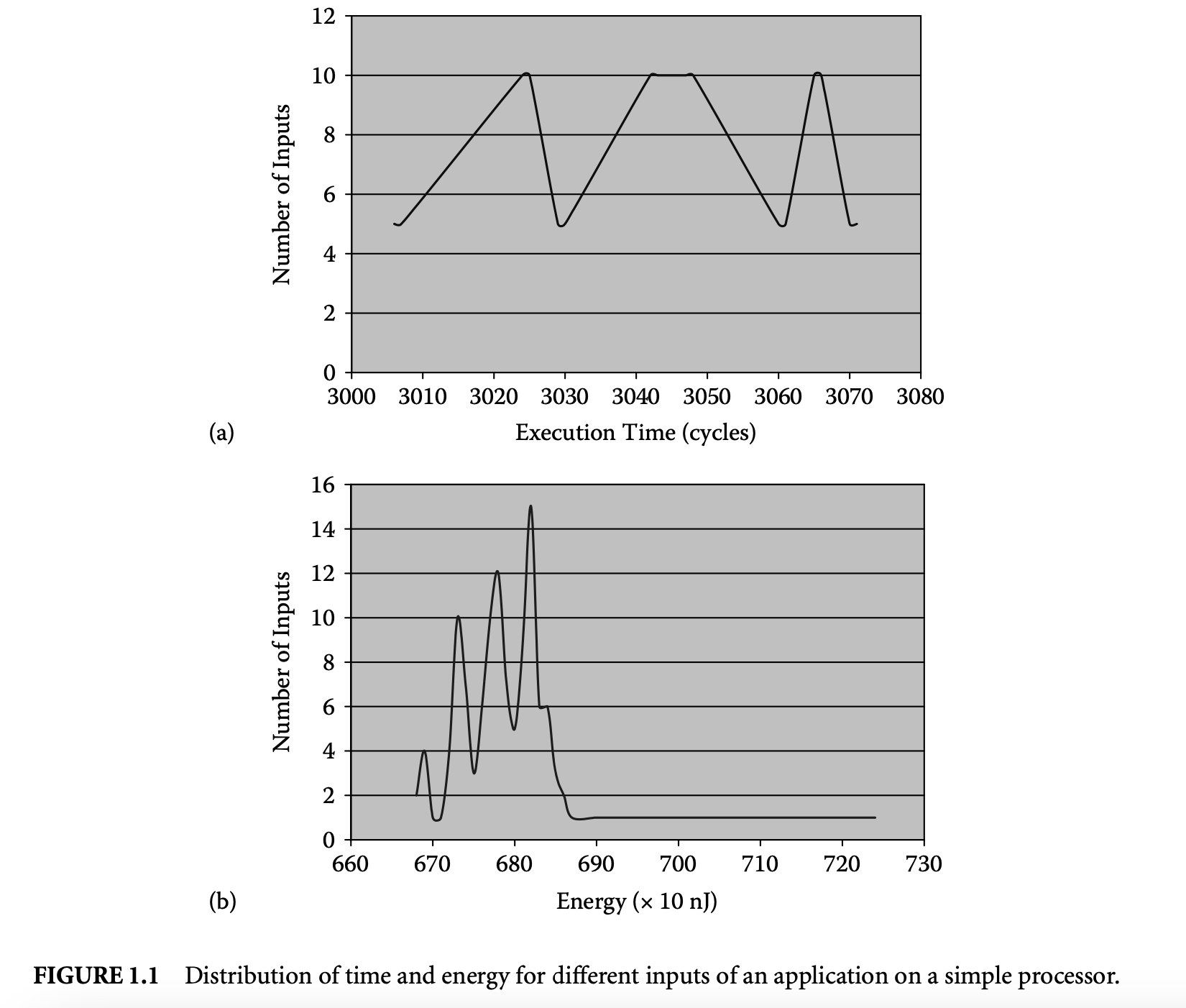
Figure 1.1a and Figure 1.2a show the variation in execution time of a program on a simple and complex processor, respectively. The program sorts a five-element array. The figures show the distribution of execution time (in processor cycles) for all possible permutations of the array elements as inputs. The maximum execution time across all the inputs is the WCET of the program. This simple example illustrates the inherent difficulty of finding the WCET value:
-
Clearly, executing the program for all possible inputs so as to bound its WCET is not feasible. The problem would be trivial if the worst-case input of a program is known a priori. Unfortunately, for most programs the worst-case input is unknown and cannot be derived easily.
-
Second, the complexity of current micro-architectures implies that the WCET is heavily influenced by the target processor. This is evident from comparing Figure 1.1a with Figure 1.2a. Therefore, the timing effects of micro-architectural components have to be accurately accounted for.
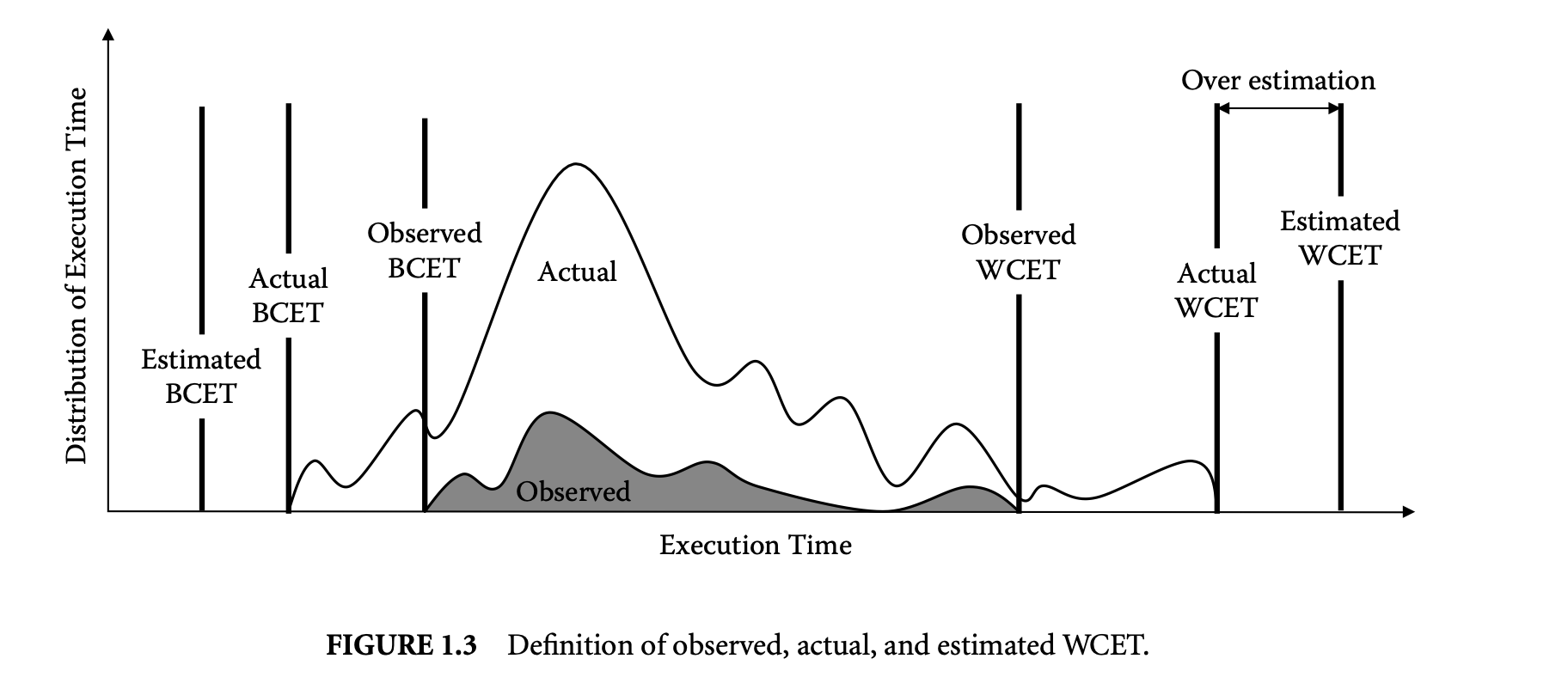
Static analysis methods estimate a bound on the WCET. These analysis techniques are conservative in nature. That is, when in doubt, the analysis assumes the worst-case behavior to guarantee the safety of the estimated value. This may lead to overestimation in some cases. Thus, the goal of static analysis methods is to estimate a safe and tight WCET value. Figure 1.3 explains the notion of safety and tightness in the context of static WCET analysis. The figure shows the variation in execution time of a task. The actual WCET is the maximum possible execution time of the program. The static analysis method generates the estimated WCET value such that estimated WCETactual WCET. The difference between the estimated and the actual WCET is the overestimation and determines how tight the estimation is. Note that the static analysis methods guarantee that the estimated WCET value can never be less than the actual WCET value. Of course, for a complex task running on a complex processor, the actual WCET value is unknown. Instead, simulation or execution of the program with a subset of possible inputs generates the observed WCET, where observed WCETactual WCET. In other words, the observed WCET value is not safe, in the sense that it cannot be used to provide absolute timing guarantees for safety-critical systems. A notion related to WCET is the BCET (best-case execution time), which represents the minimum execution time across all possible inputs. In this chapter, we will focus on static analysis techniques to estimate the WCET. However, the same analysis methods can be easily extended to estimate the BCET.
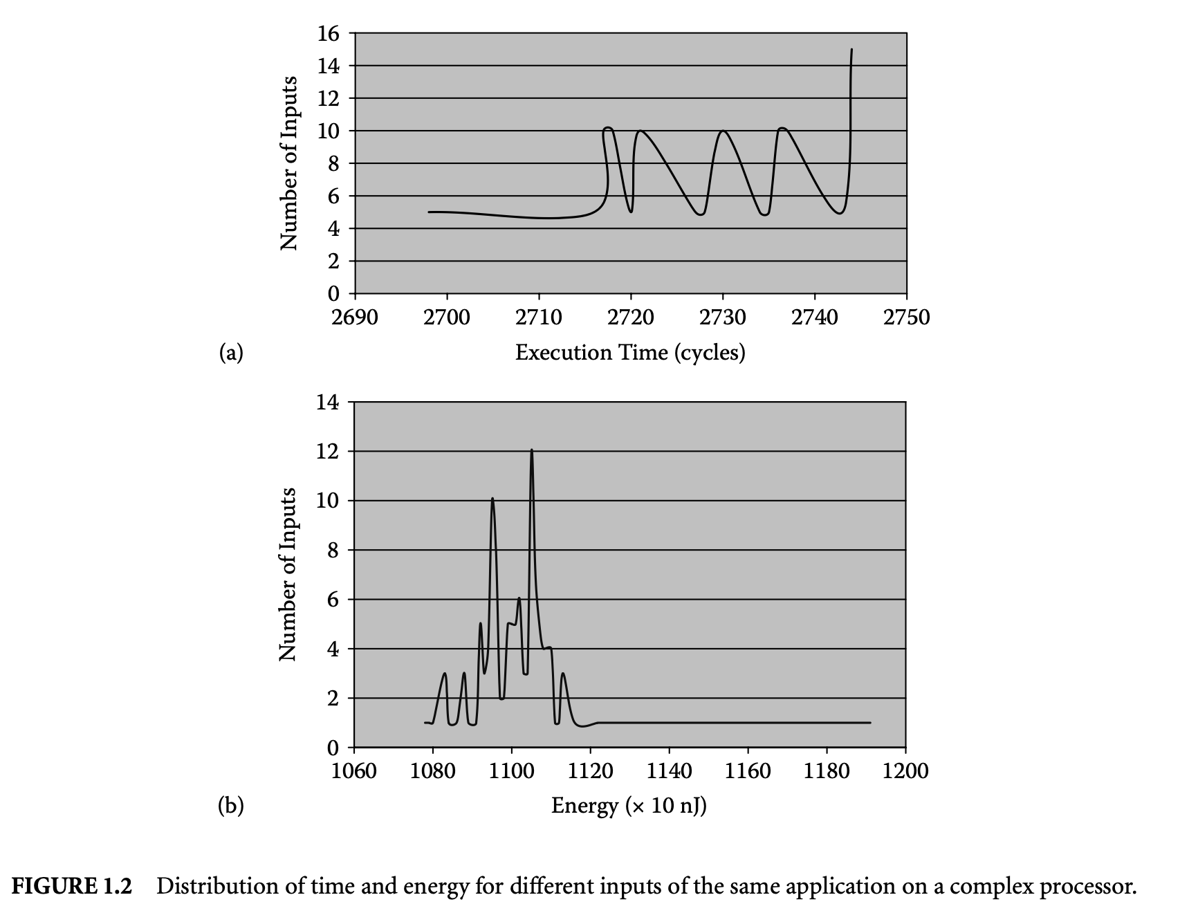
Apart from timing, the proliferation of battery-operated embedded devices has made energy consumption one of the key design constraints. Increasingly, mobile devices are demanding improved functionality and higher performance. Unfortunately, the evolution of battery technology has not been able to keep up with performance requirements. Therefore, designers of mission-critical systems, operating on limited battery life, have to ensure that both the timing and the energy constraints are satisfied under all possible scenarios. The battery should never drain out before a task completes its execution. This concern leads to the related problem of estimating the worst-case energy consumption of a task running on a processor for all possible inputs. Unlike WCET, estimating the worst-case energy remains largely unexplored even though it is considered highly important [86], especially for mobile devices. Figure 1.1b and Figure 1.2b show the variation in energy consumption of the quick sort program on a simple and complex processor, respectively.
A natural question that may arise is the possibility of using the WCET path to compute a bound on the worst-case energy consumption. As energy = average power execution time, this may seem like a viable solution and one that can exploit the extensive research in WCET analysis in a direct fashion. Unfortunately, the path corresponding to the WCET may not coincide with the path consuming maximum energy. This is made apparent by comparing the distribution of execution time and energy for the same program and processor pair as shown in Figure 1.1 and Figure 1.2. There are a large number of input pairs in this program, where , but . This happens as the energy consumed because of the switching activity in the circuit need not necessarily have a correlation with the execution time. Thus, the input that leads to WCET may not be identical to the input that leads to the worst-case energy.
The execution time or energy is affected by the path taken through the program and the underlying micro-architecture. Consequently, static analysis for worst-case execution time or energy typically consists of three phases. The first phase is the program path analysis to identify loop bounds and infeasible flows through the program. The second phase is the architectural modeling to determine the effect of pipeline, cache, branch prediction, and other components on the execution time (energy). The last phase, estimation, finds an upper bound on the execution time (energy) of the program given the results of the flow analysis and the architectural modeling.
Recently, there has been some work on measurement-based timing analysis[92, 6, 17]. This line of work is mainly targeted toward soft real-time systems, such as multimedia applications, that can afford to miss the deadline once in a while. In other words, these application domains do not require absolute timing guarantees. Measurement-based timing analysis methods execute or simulate the program on the target processor for a subset of all possible inputs. They derive the maximum observed execution time (see the definition in Figure 1.3) or the distribution of execution time from these measurements. Measurement-based performance analysis is quite useful for soft real-time applications, but they may underestimate the WCET, which is not acceptable in the context of safety-critical, hard real-time applications. In this article, we only focus on static analysis techniques that provide safe bounds on WCET and worst-case energy. The analysis methods assume uninterrupted program execution on a single processor. Furthermore, the program being analyzed should be free from unbounded loops, unbounded recursion, and dynamic function calls [67].
The rest of the chapter is organized as follows. We proceed with programming-language-level WCET analysis in the next section. This is followed by micro-architectural modeling in Section 1.3. We present a static analysis technique to estimate worst-case energy bound in Section 1.4. A brief description of existing WCET analysis tools appears in Section 1.5, followed by conclusions.
1.2 Programming-Language-Level WCET Analysis
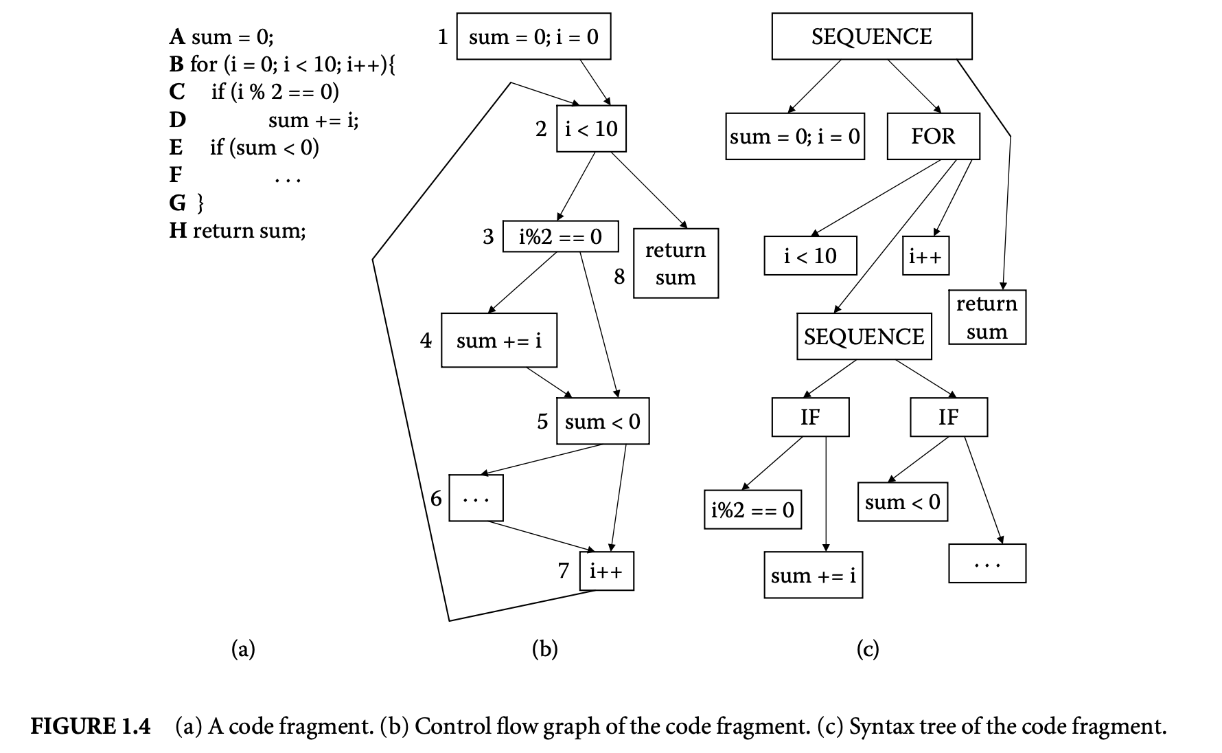
We now proceed to discuss static analysis methods for estimating the WCET of a program. For WCET analysis of a program, the first issue that needs to be determined is the program representation on which the analysis will work. Earlier works [73] have used the syntax tree where the (nonleaf) nodes correspond to programming-language-level control structures. The leaves correspond to basic blocks -- maximal fragments of code that do not involve any control transfer. Subsequently, almost all work on WCET analysis has used the control flow graph. The nodes of a control flow graph (CFG) correspond to basic blocks, and the edges correspond to control transfer between basic blocks. When we construct the CFG of a program, a separate copy of the CFG of a function is created for every distinct call site of in the program such that each call transfers control to its corresponding copy of CFG. This is how interprocedural analysis will be handled. Figure 4 shows a small code fragment as well as its syntax tree and control flow graph representations.
One important issue needs to be clarified in this regard. The control flow graph of a program can be either at the source code level or at the assembly code level. The difference between the two comes from the compiler optimizations. Our program-level analysis needs to be hooked up with micro-architectural modeling, which accurately estimates the execution time of each instruction while considering the timing effects of underlying microarchitectural features. Hence we always consider the assembly-code-level CFG. However, while showing our examples, we will show CFG at the source code level for ease of exposition.
1.2.1 WCET Calculation
We explain WCET analysis methods in a top-down fashion. Consequently, at the very beginning, we present WCET calculation -- how to combine the execution time estimates of program fragments to get the execution time estimate of a program. We assume that the loop bounds (i.e., the maximum number of iterations for a loop) are known for every program loop; in Section 2 we outline some methods to estimate loop bounds.
In the following, we outline the three main categories of WCET calculation methods. The path-based and integer linear programming methods operate on the program's control flow graph, while the tree-based methods operate on the program's syntax tree.
1.2.1.1 Tree-Based Methods
One of the earliest works on software timing analysis was the work on timing schema[73]. The technique proceeds essentially by a bottom-up pass of the syntax tree. During the traversal, it associates an execution time estimate for each node of the tree. The execution time estimate for a node is obtained from the execution time estimates of its children, by applying the rules in the schema. The schema prescribes rules -- one for each control structure of the programming language. Thus, rules corresponding to a sequence of statements, if-then-else and while-loop constructs, can be described as follows.
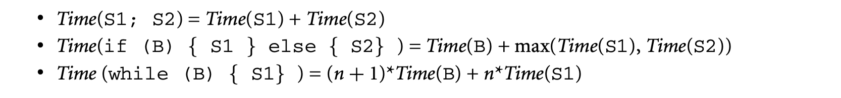
Here, is the loop bound. Clearly, S1, S2 can be complicated code fragments whose execution time estimates need to obtained by applying the schema rules for the control structures appearing in S1, S2. Extensions of the timing schema approach to consider micro-architectural modeling will be discussed in Section 1.3.5.
The biggest advantage of the timing schema approach is its simplicity. It provides an efficient compositional method for estimating the WCET of a program by combining the WCET of its constituent code fragments. Let us consider the following schematic code fragment . For simplicity of exposition, we will assume that all assignments and condition evaluations take one time unit.
i = 0; while (i<100) {if (B') S1 else S2; i++;}
If , by using the rule for if-then-else statements in the timing schema we get

Now, applying the rule for while-loops in the timing schema, we get the following. The loop bound in this case is 100.
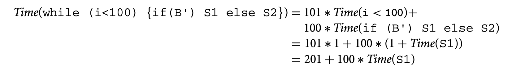
Finally, using the rule for sequential composition in the timing schema we get

The above derivation shows the working of the timing schema. It also exposes one of its major weaknesses. In the timing schema, the timing rules for a program statement are local to the statement; they do not consider the context with which the statement is arrived at. Thus, in the preceding we estimated the maximum execution time of if (B') S1 else S2 by taking the execution time for evaluating B and the time for executing S1 (since time for executing S1 is greater than the time for executing S2). As a result, since the if-then-else statement was inside a loop, our maximum execution time estimate for the loop considered the situation where S1 is executed in every loop iteration (i.e., the condition B' is evaluated to true in every loop iteration).
However, in reality S1 may be executed in very few loop iterations for any input; if Time(S1) is significantly greater than Time(S2), the result returned by timing schema will be a gross overestimate. More importantly, it is difficult to extend or augment the timing schema approach so that it can return tighter estimates in such situations. In other words, even if the user can provide the information that "it is infeasible to execute S1 in every loop iteration of the preceding program fragment ," it is difficult to exploit such information in the timing schema approach. Difficulty in exploiting infeasible program flows information (for returning tighter WCET estimates) remains one of the major weaknesses of the timing schema. We will revisit this issue in Section 1.2.2.
1.2.1.2 Path-Based Methods
The path-based methods perform WCET calculation of a program via a longest-path search over the control flow graph of . The loop bounds are used to prevent unbounded unrolling of the loops. The biggest disadvantage of this method is its complexity, as in the worst-case it may amount to enumeration of all program paths that respect the loop bounds. The advantage comes from its ability to handle various kinds of flow information; hence, infeasible path information can be easily integrated with path-based WCET calculation methods.
One approach for restricting the complexity of longest-path searches is to perform symbolic state exploration (as opposed to an explicit path search). Indeed, it is possible to cast the path-based searches for WCET calculation as a (symbolic) model checking problem [56]. However, because model checking is a verification method [13], it requires a temporal property to verify. Thus, to solve WCET analysis using model-checking-based verification, one needs to guess possible WCET estimates and verify that these estimates are indeed WCET estimates. This makes model-checking-based approaches difficult to use (see [94] for more discussion on this topic). The work of Schuele and Schneider [72] employs a symbolic exploration of the program's underlying transition system for finding the longest path, without resorting to checking of a temporal property. Moreover, they [72] observe that for finding the WCET there is no need to (even symbolically) maintain data variables that do not affect the program's control flow; these variables are identified via program slicing. This leads to overall complexity reduction of the longest-path search involved in WCET calculation.
A popular path-based WCET calculation approach is to employ an explicit longest-path search, but over a fragment of the control flow graph [31, 76, 79]. Many of these approaches operate on an acyclic fragment of the control flow graph. Path enumeration (often via a breadth-first search) is employed to find the longest path within the acyclic fragment. This could be achieved by a weighted longest-path algorithm (the weights being the execution times of the basic blocks) to find the longest sequence of basic blocks in the control flow graph for a program fragment. The longest-path algorithm can be obtained by a variation of Dijkstra's shortest-path algorithm [76]. The longest paths obtained in acyclic control flow graph fragments are then combined with the loop bounds to yield the program's WCET. The path-based approaches can readily exploit any known infeasible flow information. In these methods, the explicit path search is pruned whenever a known infeasible path pattern is encountered.
Integer Linear Programming (ILP)ILP combines the advantages of the tree and path-based approaches. It allows (limited) integration of infeasible path information while (often) being much less expensive than the path-based approaches. Many existing WCET tools such as aiT [1] and Chronos [44] employ ILP for WCET calculation.
The ILP approach operates on the program's control flow graph. Each basic block in the control flow graph is associated with an integer variable , denoting the total execution count of basic block . The program's WCET is then given by the (linear) objective function

where is the set of basic blocks of the program, and is a constant denoting the WCET estimate of basic block . The linear constraints on are developed from the flow equations based on the control flow graph. Thus, for basic block ,

where () is an ILP variable denoting the number of times control flows through the control flow graph edge (). Additional linear constraints are also provided to capture loop bounds and any known infeasible path information.
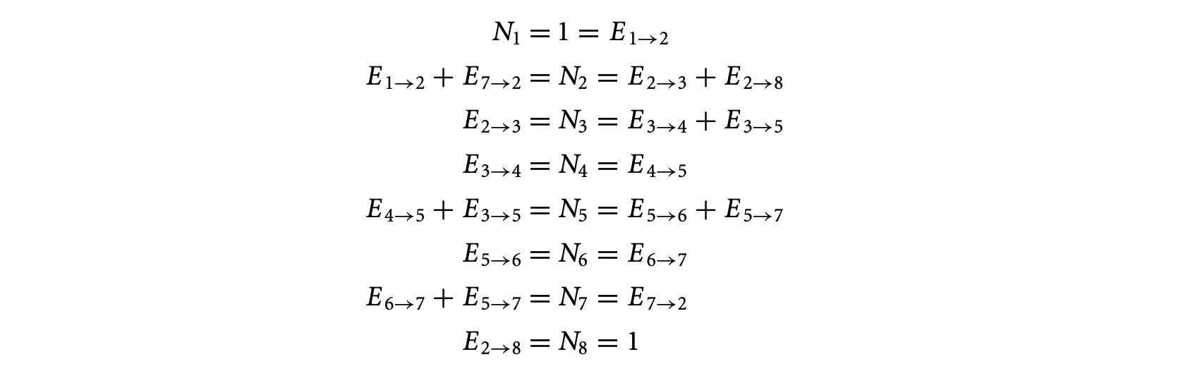
In the example of Figure 1.4, the control flow equations are given as follows. We use the numbering of the basic blocks to shown in Figure 1.4. Let us examine a few of the control flow equations. For basic block , there are no incoming edges, but there is only one outgoing edge . This accounts for the constraint ; that is, the number of executions of basic block is equal to the number of flowsfrom basic block 1 to basic block 2. In other words, whenever basic block 1 is executed, control flows from basic block 1 to basic block 2. Furthermore, since basic block 1 is the entry node, it is executed exactly once; this is captured by the constraint . Now, let us look at the constraints for basic block 2; the inflows to this basic block are the edges and and the outflows are the edges and . This means that whenever block 2 is executed, control must have flown in via either the edge or the edge ; this accounts for the constraint . Furthermore, whenever block 2 is executed, control must flow out via the edge or the edge . This accounts for the constraint . The inflow/outflow constraints for the other basic blocks are obtained in a similar fashion. The full set of inflow/outflow constraints for Figure 4 are shown in the following.
The execution time of the program is given by the following linear function in variables ( is a constant denoting the WCET of basic block ).

Now, if we ask the ILP solver to maximize this objective function subject to the inflow/outflow constraints, it will not succeed in producing a time bound for the program. This is because the only loop in the program has not been bounded. The loop bound information itself must be provided as linear constraints. In this case, since Figure 4 has only one loop, this accounts for the constraint

Using this loop bound, the ILP solver can produce a WCET bound for the program. Of course, the WCET bound can be tightened by providing additional linear constraints capturing infeasible path information; the flow constraints by default assume that all paths in the control flow graph are feasible. It is worthwhile to note that the ILP solver is capable of only utilizing the loop bound information and other infeasible path information that is provided to it as linear constraints. Inferring the loop bounds and various infeasible path patterns is a completely different problem that we will discuss next.
Before moving on to infeasible path detection, we note that tight execution time estimates for basic blocks (the constants appearing in the ILP objective function) are obtained by micro-architectural modeling techniques described in Section 3. Indeed, this is how the micro-architectural modeling and program path analysis hook up in most existing WCET estimation tools. The program path analysis is done by an ILP solver; infeasible path and loop bound information are integrated with the help of additional linear constraints. The objective function of the ILP contains the WCET estimates of basic blocks as constants. These estimates are provided by micro-architectural modeling, which considers cache, pipeline, and branch prediction behavior to tightly estimate the maximum possible execution time of a basic block (where is executed in any possible hardware state and/or control flow context).
1.2.2 Infeasible Path Detection and Exploitation
In the preceding, we have described WCET calculation methods without considering that certain sequences of program fragments may be infeasible, that is, not executed on any program input. Our WCET calculation methods only considered the loop bounds to determine a program's WCET estimate. In reality, the WCET calculation needs to consider (and exploit) other information about infeasible program paths. Moreover, the loop bounds also need to be estimated through an off-line analysis. Before proceeding further, we define the notion of an infeasible path.
Definition 1.1
Given a program , let be the set of basic blocks of . Then, an infeasible path of is a sequence of basic blocks over the alphabet , such that does not appear in the execution trace corresponding to any input of .
Clearly, knowledge of infeasible path patterns can tighten WCET estimates. This is simply because the longest path determined by our favorite WCET calculation method may be an infeasible one. Our goal is to efficiently detect and exploit infeasible path information for WCET analysis. The general problem of infeasible path detection is NP-complete [2]. Consequently, any approach toward infeasible path detection is an underapproximation -- any path determined to be infeasible is indeed infeasible, but not vice versa.
It is important to note that the infeasible path information is often given at the level of source code, whereas the WCET calculation is often performed at the assembly-code-level control flow graph. Because of compiler optimizations, the control flow graph at the assembly code level is not the same as the control flow graph at the source code level. Consequently, infeasible path information that is (automatically) inferred or provided (by the user) at the source code level needs to be converted to a lower level within a WCET estimation tool. This transformation of flow information can be automated and integrated with the compilation process, as demonstrated in [40].
In the following, we discuss methods for infeasible path detection. Exploitation of infeasible path information will involve augmenting the WCET calculation methods we discussed earlier. At this stage, it is important to note that infeasible path detection typically involves a smart path search in the program's control flow graph. Therefore, if our WCET calculation proceeds by path-based methods, it is difficult to separate the infeasible path detection and exploitation. In fact, for many path-based methods, the WCET detection and exploitation will be fused into a single step. Consequently, we discuss infeasible path detection methods and along with it exploitation of these in path-based WCET calculation. Later on, we also discuss how the other two WCET calculation approaches (tree-based methods and ILP-based methods) can be augmented to exploit infeasible path information. We note here that the problem of infeasible path detection is a very general one and has implications outside WCET analysis. In the following, we only capture some works as representatives of the different approaches to solving the problem of infeasible path detection.
1.2.2.1 Data Flow Analysis
One of the most common approaches for infeasible path detection is by adapting data flow analysis [21, 27]. In this analysis, each control location in the program is associated with an environment. An environment is a mapping of program variables to values, where each program variable is mapped to a set of values, instead of a single value. The environment of a control location captures all the possible values that the program variables may assume at ; it captures variable valuations for all possible visits to . Thus, if is an integer variable, and at line 70 of the program, the environment at line 70 maps to [0.5], this means that is guaranteed to assume an integer value between 0 and 5 when line 70 is visited. An infeasible path is detected when a variable is mapped to the empty set of values at a control location.
Approaches based on data flow analysis are often useful for finding a wide variety of infeasible paths and loop bounds. However, the environments computed at a control location may be too approximate. It is important to note that the environment computed at a control location is essentially an _invariant_property -- a property that holds for every visit to . To explain this point, consider the example program in Figure 1.4a. Data flow analysis methods will infer that in line E of the program , that is, . Hence we can infer that execution of lines E, F in Figure 1.4a constitutes an infeasible path. However, by simply keeping track of all possible variable values at each control location we cannot directly infer that line D of Figure 1.4a cannot be executed in consecutive iterations of the loop.
1.2.2.2 Constraint Propagation Methods
The above problem is caused by the merger of environments at any control flow merge point in the control flow graph. The search in data flow analysis is not truly path sensitive -- at any control location we construct the environment for from the environments of all the control locations from which there is an incoming control flow to . One way to solve this problem is to perform constraint propagation [7, 71] (or value propagation as in [53]) along paths via symbolic execution. Here, instead of assigning possible values to program variables (as in flow analysis), each input variable is given a special value: unknown. Thus, if nothing is known about a variable , we simply represent it as . The operations on program variables will then have to deal with these symbolic representations of variables. The search then accumulates constraints on and detects infeasible paths whenever the constraint store becomes unsatisfiable. In the program of Figure 1.4a, by traversing lines C,D we accumulate the constraint & . In the subsequent iteration, we accumulate the constraint +1 & . Note that via symbolic execution we know that the current value of is one greater than the value in the previous iteration, so the constraint +1 & . We now need to show that the constraint & +1 & is unsatisfiable in order to show that line D in Figure 1.4a cannot be visited in subsequent loop iterations. This will require the help of external constraint solvers or theorem provers such as Simplify [74]. Whether the constraint in question can be solved automatically by the external prover, of course, depends on the prover having appropriate decision procedures to reason about the operators appearing in the constraint (such as the addition and remainder operators appearing in the constraint & + 1 & ).
The preceding example shows the plus and minus points of using path-sensitive searches for infeasible path detection. The advantage of using such searches is the precision with which we can detect infeasible program paths. The difficulty in using full-fledged path-sensitive searches (such as model checking) is, of course, the huge number of program paths to consider.1
Furthermore, the data variables of a program typically come from unbounded domains such as integers. Thus, use of a finite-state search method such as model checking will have to either employ data abstractions to construct a finite-state transition system corresponding to a program or work on symbolic state representations representing infinite domains (possibly as constraints), thereby risking nontermination of the search.
In summary, even though path-sensitive searches are more accurate, they suffer from a huge complexity. Indeed, this has been acknowledged in [53], which accommodates specific heuristics to perform path merging. Consequently, using path-sensitive searches for infeasible path detection does not scale up to large programs. Data flow analysis methods fare better in this regard since they perform merging at control flow merge points in the control flow graph. However, even data flow analysis methods can lead to full-fledged loop unrolling if a variable gets new values in every iteration of a loop (e.g., consider the program while (...){ i++ } ).
1.2.2.3 Heuristic Methods
To avoid the cost of loop unrolling, the WCET community has studied techniques that operate on the acyclic graphs representing the control flow of a single loop iteration [76, 31, 79]. These techniques do not detect or exploit infeasible paths that span across multiple loop iterations. The basic idea is to find the weighted longest path in any loop iteration and multiply its cost with the loop bound. Again, the complication arises from the presence of infeasible paths even within a loop iteration. The work of Stappert et al. [76] finds the longest path in a loop iteration and checks whether it is feasible; if is infeasible, it employsgraph-theoretic methods to remove from the control flow graph of the loop. The longest-path calculation is then run again on the modified graph. This process is repeated until a feasible longest path is found. Clearly, this method can be expensive if the feasible paths in a loop have relatively low execution times.
To address this gap, the recent work of Suhendra et al. [79] has proposed a more "infeasible path aware" search of the control flow graph corresponding to a loop body. In this work, the infeasible path detection and exploitation proceeds in two separate steps. In the first step, the work computes "conflict pairs," that is, incompatible (branch, branch) or (assignment, branch) pairs. For example, let us consider the following code fragment, possibly representing the body of a loop.

Clearly, the assignment at line 4 conflicts with the branch at line 5 evaluating to false. Similarly, the branch at line 1 evaluating to true conflicts with the branch at line 5 evaluating to true. Such conflicting pairs are detected in a traversal of the control flow directed acyclic graph (DAG) corresponding to the loop body. Subsequently, we traverse the control flow DAG of the loop body from sink to source, always keeping track of the heaviest path. However, if any assignment or branch decision appearing in the heaviest path is involved in a conflict pair, we also keep track of the next heaviest path that is not involved in such a pair. Consequently, we may need to keep track of more than one path at certain points during the traversal; however, redundant tracked paths are removed as soon as conflicts (as defined in the conflict pairs) are resolved during the traversal. This produces a path-based WCET calculation method that detects and exploits infeasible path patterns and still avoids expensive path enumeration or backtracking.
We note that to scale up infeasible path detection and exploitation to large programs, the notion of pairwise conflicts is important. Clearly, this will not allow us to detect that the following is an infeasible path:
x=1;y=x;if(y>2){...
However, using pairwise conflicts allows us to avoid full-fledged data flow analysis in WCET calculation. The work of Healy and Whalley [31] was the first to use pairwise conflicts for infeasible path detection and exploitation. Apart from pairwise conflicts, this work also detects iteration-based constraints, that is, the behavior of individual branches across loop iterations. Thus, if we have the following program fragment, the technique of Healy and Whalley [31] will infer that the branch inside the loop is true only for the iterations 0..24.
for(i=0;i<100;i++){ if(i<25){ S1;} else{ S2;} }
If the time taken to execute S1 is larger than the time taken to execute S2, we can estimate the cost of the loop to be . Note that in the absence of a framework for using iteration-based constraints, we would have returned the cost of the loop as .
In principle, it is possible to combine the efficient control flow graph traversal in [79] with the framework in [31], which combines branch constraints as well as iteration-based constraints. This can result in a path-based WCET calculation that performs powerful infeasible path detection [31] and efficient infeasible path exploitation [79].

1.2.2.4 Loop Bound Inferencing
An important part of infeasible path detection and exploitation is inferencing and usage of loop bounds. Without sophisticated inference of loop bounds, the WCET estimates can be vastly inflated. To see this point, we only need to examine a nested loop of the form shown in Figure 1.5. Here, a naive method will put the loop bound of the inner loop as , which is a gross overestimate over the actual bound of .
Initial work on loop bounds relied on the programmer to provide manual annotations [61]. These annotations are then used in the WCET calculation. However, giving loop bound annotations is in general an error-prone process. Subsequent work has integrated automated loop bound inferencing as part of infeasible path detection [21]. The work of Liu and Gomez [52] exploits the program structure for high-level languages (such as functional languages) to infer loop bounds. In this work, from the recursive structure of the functions in a functional program, a cost function is constructed automatically. Solving this cost-bound function can then yield bounds on loop executions (often modeled as recursion in functional programs). However, if the program is recursive (as is common for functional programs), the cost bound function is also recursive and does not yield a closed-form solution straightaway. Consequently, this technique [52] (a) performs symbolic evaluation of the cost-bound function using knowledge of program inputs and then (b) transforms the symbolically evaluated function to simplify its recursive structure. This produces the program's loop bounds. The technique is implemented for a subset of the functional language Scheme.2
Dealing loops as recursive procedures has also been studied in [55] but in a completely different context. This work uses context-sensitive interprocedural analysis to separate out the cache behavior of different executions of the recursive procedure corresponding to a loop, thereby distinguishing, for instance, the cache behavior of the first loop iteration from the remaining loop iterations.
Footnote 2: Dealing loops as recursive procedures has also been studied in [55] but in a completely different context. This work uses context-sensitive interprocedural analysis to separate out the cache behavior of different executions of the recursive procedure corresponding to a loop, thereby distinguishing, for instance, the cache behavior of the first loop iteration from the remaining loop iterations.
For imperative programs, the work of Healy et al. [30] presents a comprehensive study for inferring loop bounds of various kinds of loops. It handles loops with multiple exits by automatically identifying the conditional branches within a loop body that may affect the number of loop iterations. Subsequently, for each of these branches the range of loop iterations where they can appear is detected; this information is used to compute the loop bounds. Moreover, the work of Healy et al. [30] also presents techniques for automatically inferring bounds on loops where loop exit/entry conditions depend on values of program variables. As an example, let us consider the nonrectangular loop nest shown in Figure 1.5. The technique of Healy et al. [30] will automatically extract the following expression for the bound on the number of executions of the inner loop.

We can then employ techniques for solving summations to obtain .
1.2.2.5 Exploiting Infeasible Path Information in Tree-Based WCET Calculation
So far, we have outlined various methods for detecting infeasible paths in a program's control flow graph. These methods work by traversing the control flow graph and are closer to the path-based methods.
Figure 1.5: A nonrectangular loop nest.
If the WCET calculation is performed by other methods (tree based or ILP), how do we even integrate the infeasible path information into the calculation? In other words, if infeasible path patterns have been detected, how do we let tree-based or ILP-based WCET calculation exploit these patterns to obtain tighter WCET bounds? We first discuss this issue for tree-based methods and then for ILP methods.
One simple way to exploit infeasible path information is to partition the set of program inputs. For each input partition, the program is partially evaluated to remove the statements that are never executed (for inputs in that partition). Timing schema is applied to this partially evaluated program to get its WCET. This process is repeated for every input partition, thereby yielding a WCET estimate for each input partition. The program's WCET is set to the maximum of the WCETs for all the input partitions. To see the benefit of this approach, consider the following schematic program with a boolean input b.

Assume that

Then using the rules of timing schema we have the following. For convenience, we call the first (second) if statement in the preceding schematic program fragment If Stmt(If Stmt).
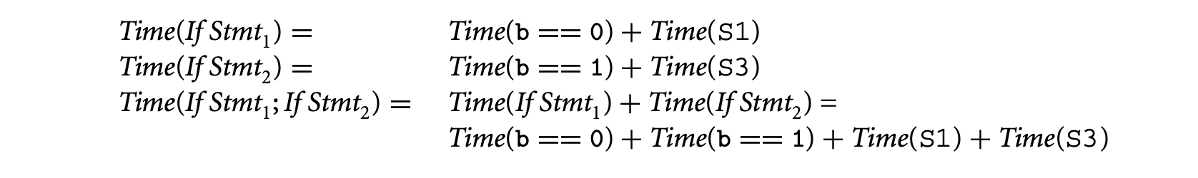
We now consider the execution time for the two possible inputs and take their maximum. Let us now consider the program for input b = 0. Since statements S1 and S4 are executed, we have:

Similarly, S2 and S3 are executed for b = 1. Thus,

The execution time estimate is set to the maximum of and . Both of these quantities are lower than the estimate computed by using the default timing schema rules. Thus, by taking the maximum of these two quantities we will get a tighter estimate than by applying the vanilla timing schema rules.
Partitioning the program inputs and obtaining the WCET for each input partition is a very simple, yet powerful, idea. Even though it has been employed for execution time analysis and energy optimization in the context of timing schema [24, 25], we can plug this idea into other WCET calculation methods as well. The practical difficulty in employing this idea is, of course, computing the input partitions in general. In particular, Gheorghita et al. [25] mention the suitability of the input partitioning approach for multimedia applications performing video and audio decoding and encoding; in these applications there are different computations for different types of input frames being decoded and encoded. However, in general, it is difficult to partition the input space of a program so that inputs with similar execution time estimates get grouped to the same partition. As an example, consider the insertion sort program where the input space consists of the different possible ordering of the input elements in the input array. Thus, in an -element input array, the input space consists of the different possible permutations of the array element (the permutation denoting the ordering ). First, getting such a partitioning will involve an expensive symbolic execution of the sorting program. Furthermore, even after we obtain the partitioning we still have too many input partitions to work with (the number of partitions for the sorting program is the number of permutations, that is, ). In the worst case, each program input is in a different partition, so the WCET estimation will reduce to exhaustive simulation.
A general approach for exploiting infeasible path information in tree-based WCET calculation has been presented in [61]. In this work, the set of all paths in the control flow graph (taking into account the loop bounds) is described as a regular expression. This is always possible since the set of paths in the control flow graph (taking into account the loop bounds) is finite. Furthermore, all of the infeasible path information given by the user is also converted to regular expressions. Let Paths be the set of all paths in the control flow graph and let , be certain infeasible path information (expressed as a regular expression). We can then safely describe the set of feasible paths as ; this is also a regular expression since regular languages are closed under negation and intersection. Timing schema now needs to be employed in these paths, which leads to a practical difficulty. To explain this point, consider the following simple program fragment.

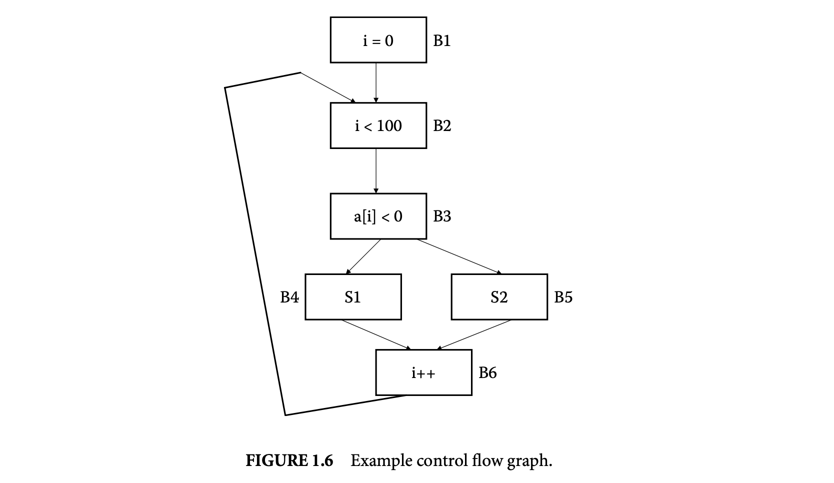
We can draw the control flow graph of this program and present the set of paths in the control flow graph (see Figure 6) as a regular expression over basic block occurrences. Thus, the set of paths in the control flow graph fragment of Figure 6 is

Now, suppose we want to feed the information that the block B4 is executed at least in one iteration. If is an input array, this information can come from our knowledge of the program input. Alternatively, if was constructed via some computation prior to the loop, this information can come from our understanding of infeasible program paths. In either case, the information can be encoded as the regular expression , where is the set of all basic blocks. The set of paths that the WCET analysis should consider is now given by

The timing schema approach will now remove the intersection by unrolling the loop as follows.
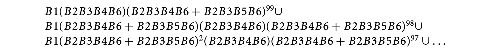
For each of these sets of paths (whose union we represent above) we can employ the conventional timing schema approach. However, there are 100 sets to consider because of unrolling a loop with 100 iterations. This is what makes the exploitation of infeasible paths difficult in the timing schema approach.
1.2.2.6 Exploiting Infeasible Path Information in ILP-Based WCET Calculation
Finally, we discuss how infeasible path information can be exploited in the ILP-based approach for WCET calculation. As mentioned earlier, the ILP-based approach is the most widely employed WCET calculation approach in state-of-the-art WCET estimation tools. The ILP approach reduces the WCET calculation to a problem of optimizing a linear objective function. The objective function represents the execution time of the program, which is maximized subject to flow constraints (in the control flow graph) and loop bound constraints. Note that the variables in the ILP problem correspond to execution counts of control flow graph nodes (i.e., basic blocks and edges).
Clearly, integrating infeasible path information will involve encoding knowledge of infeasible program paths as additional linear constraints [49, 68]. Introducing such constraints will make the WCET estimate (returned by the ILP solver) tighter. The description of infeasible path information as linear constraints has been discussed in several works. Park proposes an information description language (IDL) for describing infeasible path information [62]. This language provides convenient primitives for describing path information through annotations such as sampetth(A,C), where can be lines in the program. This essentially means than whenever is executed, is executed and vice versa (note that can be executed many times, as they may lie inside a loop). In terms of execution count constraints, such information can be easily encoded as , where and are the basic blocks containing , and and are the number of executions of and .
Recent work [e.g., 20] provides a systematic way of encoding path constraints as linear constraints on execution counts of control flow graph nodes and edges. In this work, the program's behavior is described in terms of "scopes"; scope boundaries are defined by loop or function call entry and exit. Within each scope, the work provides a systematic syntax for providing path information in terms of linear constraints.
For example, let us consider the control flow graph schematic denoting two if-then-else statements within a loop shown in Figure 7. The path information is now given in terms of each/all iterations of the scope (which in this case is the only loop in Figure 7). Thus, if we want to give the information that blocks and are always executed together (which is equivalent to using the sampetth annotation described earlier) we can state it as . On the other hand, if we want to give the information that B2 and B6 are never executed together (in any iteration of the loop), this gets converted to the following format

Incorporating the number of loop iterations in the above constraints, one can obtain the linear constraint (assuming that the loop bound is 100). This constraint is then fed to the ILP solver along with the flow constraints and loop bounds (and any other path information).
In conclusion, we note that the ILP formulation for WCET calculation relies on aggregate execution counts of basic blocks. As any infeasible path information involves sequences of basic blocks, the encoding of infeasible path information as linear constraints over aggregate execution counts can lose information (e.g., it is possible to satisfy in a loop with 100 iterations even if and are executed together in certain iterations). However, encoding infeasible path information as linear constraints provides a safe and effective way of ruling out a wide variety of infeasible program flows. Consequently, in most existing WCET estimation tools, ILP is the preferred method for WCET calculation.

1.3 Micro-Architectural Modeling
The execution time of a basic block in a program executing on a particular processor depends on (a) the number of instructions in , (b) the execution cycles per instruction in , and (c) the clock period of the processor. Let a basic block contain the sequence of instructions . For a simple micro-controller (e.g., TI MSP430), the execution latency of any instruction type is a constant. Let be a constant denoting the execution cycles of instruction . Then the execution time of the basic block can be expressed as
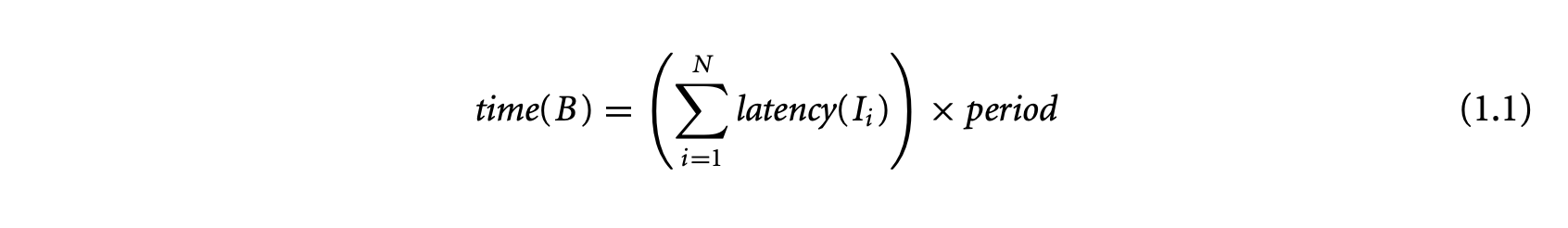
where is the clock period of the processor. Thus, for a simple micro-controller, the execution time of a basic block is also a constant and is trivial to compute. For this reason, initial work on timing analysis [67, 73] concentrated mostly on program path analysis and ignored the processor architecture.
However, the increasing computational demand of the embedded systems led to the deployment of processors with complex micro-architectural features. These processors employ aggressive pipelining, caching, branch prediction, and other features [33] at the architectural level to enhance performance. While the increasing architectural complexity significantly improves the average-case performance of an application, it leads to a high degree of timing unpredictability. The execution cycle of an instruction in Equation 1.1 is no longer a constant; instead it depends on the execution context of the instruction. For example, in the presence of a cache, the execution time of an instruction depends on whether the processor encounters a cache hit or a cache misses while fetching the instruction from the memory hierarchy. Moreover, the large difference between the cache hit and miss latency implies that assuming all memory accesses to be cache misses will lead to overly pessimistic timing estimates. Any effective estimation technique should obtain a safe but tight bound on the number of cache misses.
1.3.1 Sources of Timing Unpredictability
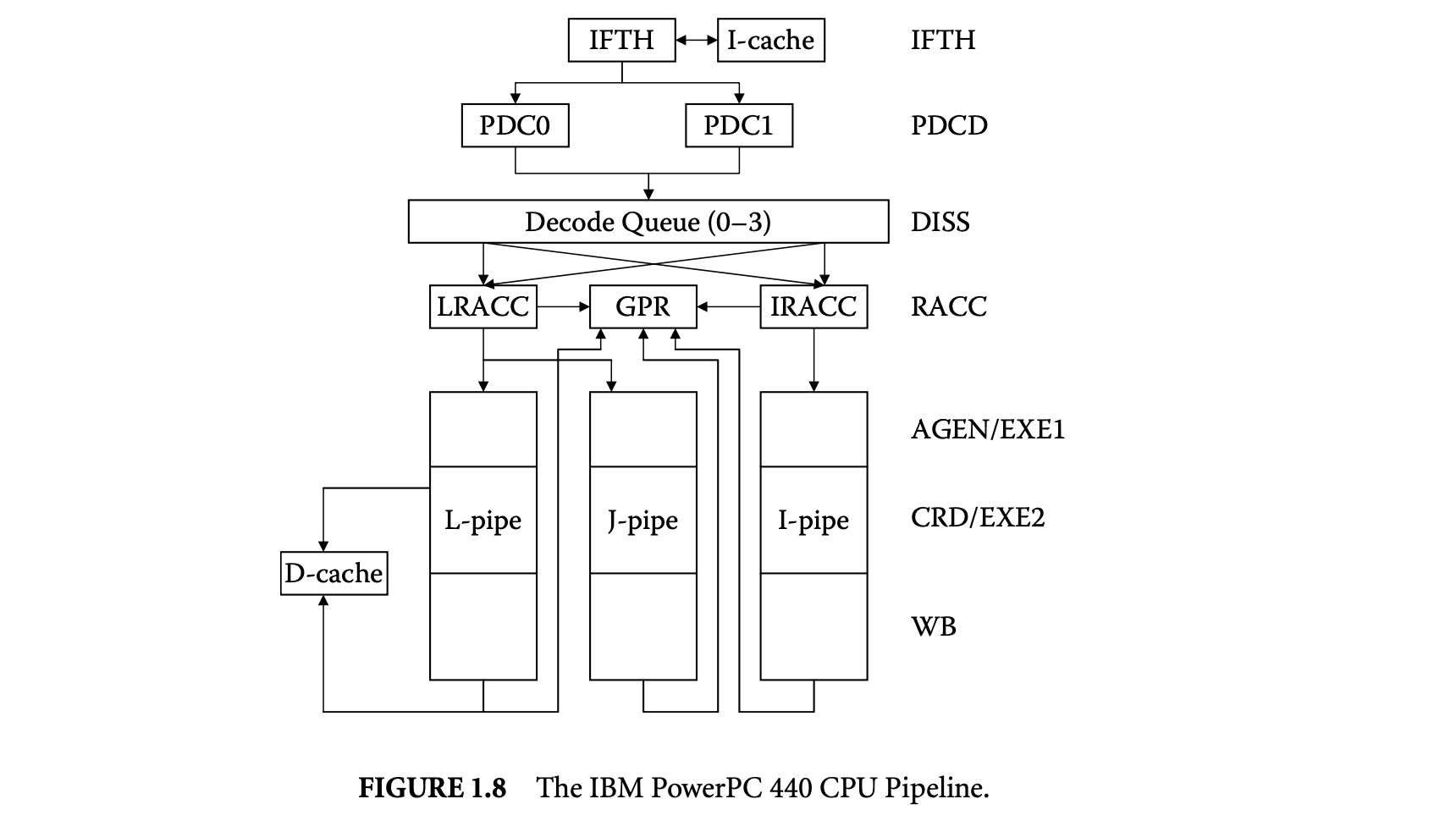
We first proceed to investigate the sources of timing unpredictability in a modern processor architecture and their implications for timing analysis. Let us use the IBM PowerPC (PPC) 440 embedded core [34] for illustration purposes. The PPC 440 is a 32-bit RISC CPU core optimized for embedded applications. It integrates a superscalar seven-stage pipeline, with support for out-of-order issue of two instructions per clock to multiple execution units, separate instruction and data caches, and dynamic branch prediction.
Figure 8 shows the PPC 440 CPU pipeline. The instruction fetch stage (IFTH) reads a cache line (two instructions) into the instruction buffer. The predecode stage (PDCD) partially decodes at most two instructions per cycle. At this stage, the processor employs a combination of static and dynamic branch prediction for conditional branches. The four-entry decode queue accepts up to two instructions per cycle from the predecode stage and completes the decoding. The decode queue always maintains the instructions in program order. An instruction waits in the decode queue until its input operands are ready and the corresponding execution pipeline is available. Up to two instructions can exit the decode queue per cycle and are issued to the register access (RACC) stage. Instruction can be issued out-of-order from the decode queue. After register access, the instructions proceed to the execution pipelines. The PPC 440 contains three execution pipelines: a load/store pipe, a simple integer pipe, and a complex integer pipe. The first execute stage (AGEN/EXE1) completes simple arithmetics and generates load/store addresses. The second execute stage (CRD/EXE2) performs data cache access and completes complex operations. The write back (WB) stage writes back the results into the register file.
Ideally, the PPC 440 pipeline has a throughput of two instructions per cycle. That is, the effective latency of each individual instruction is 0.5 clock cycle. Unfortunately, most programs encounter multiple pipeline hazards during execution that introduce bubbles in the pipeline and thereby reduce the instruction throughput:
Cache miss:: Any instruction may encounter a miss in the instruction cache (IFTH stage) and the load/store instructions may encounter a miss in the data cache (CRD/EXE2 stage). The execution of the instruction gets delayed by the cache miss latency. Data dependency:: Data dependency among the instructions may introduce pipeline bubbles. An instruction dependent on another instruction for its input operand has to wait in the decode queue until produces the result.
Control dependency:: Control transfer instructions such as conditional branches introduce control dependency in the program. Conditional branch instructions cause pipeline stalls, as the processor does not know which way to go until the branch is resolved. To avoid this delay, dynamic branch prediction in the PPC 440 core predicts the outcome of the conditional branch and then fetches and executes the instructions along the predicted path. If the prediction is correct, the execution proceeds without any delay. However, in the event of a misprediction, the pipeline is flushed and a branch misprediction penalty is incurred.
Resource contention:: The issue of an instruction from the decode queue depends on the availability of the corresponding execution pipeline. For example, if we have two consecutive load/store instructions in the decode queue, then only one of them can be issued in any cycle.
Pipeline hazards have significant impact on the timing predictability of a program. Moreover, certain functional units may have variable latency, which is input dependent. For example, the PPC 440 core can be complemented by a floating point unit (FPU) for applications that need hardware support for floating point operations [16]. In that case, the latency of an operation can be data dependent. For example, to mitigate the long latency of the floating point divide (19 cycles for single precision), the PPC 440 FPU employs an iterative algorithm that stops when the remainder is zero or the required target precision has been reached. A similar approach is employed for integer divides in some processors. In general, any unit that complies with the IEEE floating point standard [35] introduces several sources for variable latency (e.g., normalized versus denormalized numbers, exceptions, multi-path adders, etc.).
A static analyzer has to take into account the timing effect of these various architectural features to derive a safe and tight bound on the execution time. This, by itself, is a difficult problem.
1.3.2 Timing Anomaly
The analysis problem becomes even more challenging because of the interaction among the different architectural components. These interactions lead to counterintuitive timing behaviors that essentially preclude any compositional analysis technique to model the components independently.
Timing anomaly is a term introduced to define the counterintuitive timing behavior [54]. Let us assume a sequence of instructions executing on an architecture starting with an initial processor state. The latency of the first instruction is modified by an amount . Let be the resulting change in the total execution time of the instruction sequence.
Definition 1.2: A timing anomaly is a situation where one the following cases becomes true:

From the perspective of WCET analysis, the cases of concern are the following: (a) The (local) worst-case latency of an instruction does not correspond to the (global) WCET of the program (e.g., results in ), and (b) the increase in the global execution time exceeds the increase in the local instruction latency (e.g., results in ). Most analysis techniques implicitly assume that the worst-case latency of an instruction will lead to safe WCET estimates. For example, if the cache state is unknown, it is common to assume a cache miss for an instruction. Unfortunately, in the presence of a timing anomaly, assuming a cache miss may lead to underestimation.
1.3.2.1 Examples
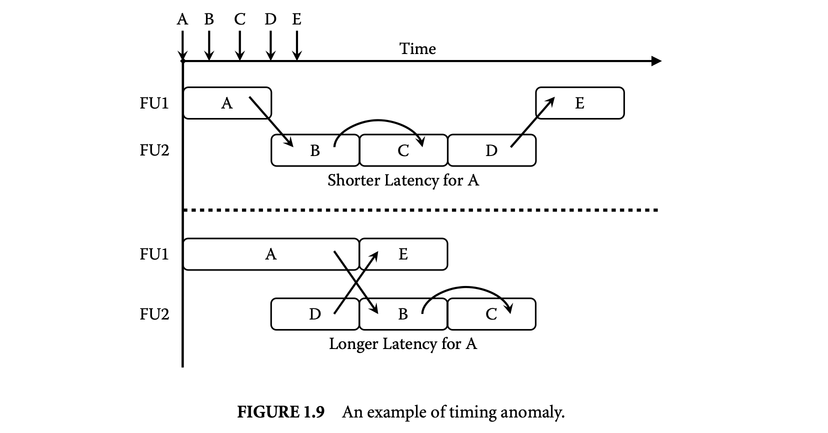
An example where the local worst case does not correspond to the global worst case is illustrated in Figure 1.9. In this example, instructions A, E execute on functional unit 1 (FU1), which has variable latency. Instructions B, C, and D execute on FU2, which has a fixed latency. The arrows on the time line show when each instruction becomes ready and starts waiting for the functional unit. The processorallows out-of-order issue of the ready instructions to the functional units. The dependencies among the instructions are shown in the figure. In the first scenario, instruction A has a shorter latency, but the schedule leads to longer total execution time, as it cannot exploit any parallelism. In the second scenario, A has longer latency, preventing B from starting execution earlier (B is dependent on A). However, this delay opens up the opportunity for D to start execution earlier. This in turn allows E (which is dependent on D) to execute in parallel with B and C. The increased parallelism results in shorter overall execution time for the second scenario even though A has longer latency.
The second example illustrates that the increase in the global execution time may exceed the increase in the local instruction latency. In the PPC 440 pipeline, the branch prediction can indirectly affect instruction cache performance. As the processor caches instructions along the mispredicted path, the instruction cache content changes. This is called wrong-path instructions prefetching[63] and can have both constructive and destructive effects on the cache performance. Analyzing each feature individually fails to model this interference and therefore risks missing out on corner cases where branch misprediction introduces additional cache misses.
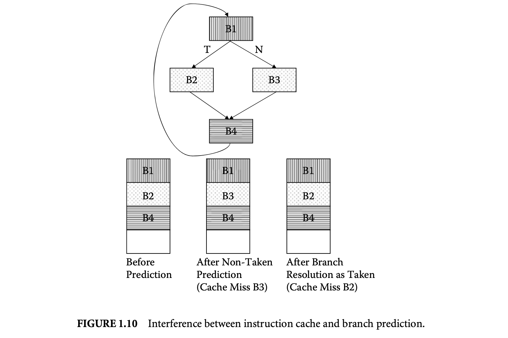
This is illustrated in Figure 10 with an example control flow graph. For simplicity of exposition, let us assume an instruction cache with four lines (blocks) where each basic block maps to a cache block (in reality, a basic block may get mapped to multiple cache blocks or may occupy only part of a cache block). Basic block B1 maps to the first cache block, B4 maps to the third cache block, and B2 and B3 both map to the second cache block (so they can replace each other). Suppose the execution sequence is B1 B2 B4 B1 B2 B4 B1 B2 B4... That is, the conditional branch at the end of B1 is always taken; however, it is always mispredicted. The conditional branch at the end of B4, on the other hand, is always correctly predicted. If we do not take branch prediction into account, any analysis technique will conclude a cache hit for all the basic blocks for all the iterations except for the first iteration (which encounters cold misses). Unfortunately, this may lead to underestimation in the presence of branch prediction. The cache state before the prediction at B1 is shown in Figure 10. The branch is mispredicted, leading to instruction fetch along B3. Basic block B3 incurs a cache miss and replaces B2. When the branch is resolved, however, B2 is fetched into the instruction cache after another cache miss. This will result in two additional cache misses per loop iteration. In this case, the total increase in execution time exceeds the branch misprediction penalty because of the additional cache misses. Clearly, separate analysis of instruction caches and branch prediction cannot detect these additional cache misses.
Interested readers can refer to [54] for additional examples of timing anomalies based on a simplified PPC 440 architecture. In particular, [54] presents examples where (a) a cache hit results in worst-case timing, (b) a cache miss penalty can be higher than expected, and (c) the impact of a timing anomaly on WCET may not be bounded. The third situation is the most damaging, as a small delay at the beginning of execution may contribute an arbitrarily high penalty to the overall execution time through a domino effect.
Identifying the existence and potential sources of a timing anomaly in a processor architecture remains a hard problem. Lundqvist and Stenstrom [54] claimed that no timing anomalies can occur if a processor contains only in-order resources, but Wenzel et al. [91] constructed an example of a timing anomaly in an in-order superscalar processor with multiple functional units serving an overlapping set of instruction types. A model-checking-based automated timing anomaly identification method has been proposed [18] for a simplified processor. However, the scalability of this method for complex processors is not obvious.
1.3.2.2 Implications
Timing anomalies have serious implications for static WCET analysis. First, the anomaly caused by scheduling (as shown in Figure 1.9) implies that one has to examine all possible schedules of a code fragment to estimate the longest execution time. A sequence of instructions, where each instruction can have possible latency values, generates schedules. Any static analysis technique that examines all possible schedules will have prohibitive computational complexity. On the other hand, most existing analysis methods rely on making safe local decisions at the instruction level and hence run the risk of underestimation.
Second, many analysis techniques adopt a compositional approach to keep the complexity of the modeling architecture under control [81, 29]. These approaches model the timing effects of the different architectural features in separation. Counterintuitive timing interference among the different features (e.g., cache and branch prediction in Figure 1.10 or cache and pipeline) may render the compositional approaches invalid. For example, Healy et al. [29] performed cache analysis followed by pipeline analysis. Whenever a memory block cannot be classified as a cache hit or miss, it is assumed to be a cache miss. This is a conservative decision in the context of cache modeling and works perfectly for the in-order processor pipeline modeled in that work. However, if it is extended to out-of-order pipeline modeling, the cache hit may instead result in worst-case timing, and the decision will not be safe.
Lundqvist and Stenstrom [54] propose a program modification method that enforces timing predictability and thereby simplifies the analysis. For example, any variable latency instruction can be preceded and succeeded by "synchronization" instructions to force serialization. Similarly, synchronization instructions and/or software-based cache prefetching can be introduced at program path merging points to ensure identical processor states, but this approach has a potentially high performance overhead and requires special hardware support.
An architectural approach to avoid complex analysis due to timing anomalies has been presented in [3]. An application is divided into multiple subtasks with checkpoints to monitor the progress. The checkpoints are inserted based on a timing analysis of a simple processor pipeline (e.g., no out-of-order execution, branch prediction, etc.). The application executes on a complex pipeline unless a subtask fails to complete before its checkpoint (which is rare). At this point, the pipeline is reconfigured to the simple mode so that the unfinished subtasks can complete in a timely fashion. However, this approach requires changes to the underlying processor micro-architecture.
1.3.3 Overview of Modeling Techniques
The micro-architectural modeling techniques can be broadly divided into two groups:
- Separated approaches
- Integrated approaches
The separated approaches work on the control flow graph, estimating the WCET of each basic block by using micro-architectural modeling. These WCET estimates are then fed to the WCET calculation method. Thus, if the WCET calculation proceeds by ILP, only the constants in the ILP problem corresponding to the WCET of the basic blocks are obtained via micro-architectural modeling.
In contrast, the integrated approaches work by augmenting a WCET calculation method with micro-architectural modeling. In the following we see at least two such examples -- an augmented ILP modeling method (to capture the timing behavior of caching and branch prediction) and an augmented timing schema approach that incorporates cache/pipeline modeling. Subsequently, we will discuss two examples of separated approaches, one of them using abstract interpretation for the micro-architectural modeling and the other one using a customized fixed-point analysis over the time intervals at which events (changing pipeline state) can occur. In both examples of the separated approach, the program path analysis proceeds by ILP.
In addition, there exist static analysis methods based on symbolic execution of the program [53]. This is an integrated method that extends cycle-accurate architectural simulation to perform symbolic execution with partially known operand values. The downside of this approach is the slow simulation speed that can lead to long analysis time.
1.3.4 Integrated Approach Based on ILP
An ILP-based path analysis technique has been described in Section 2.2. Here we present ILP-based modeling of micro-architectural components. In particular, we will focus on ILP-based instruction cache modeling proposed in [50] and dynamic branch prediction modeling proposed in [45]. We will also look at modeling the interaction between the instruction cache and the branch prediction [45] to capture the wrong-path instruction prefetching effect discussed earlier (see Figure 1.10).
The main advantage of ILP-based WCET analysis is the integration of path analysis and micro-architectural modeling. Identifying the WCET path is clearly dependent on the timing of each individual basic block, which is determined by the architectural modeling. On the other hand, behavior of instruction cache and branch prediction depends heavily on the current path. In other words, unlike pipeline, timing effects of cache and branch prediction cannot be modeled in a localized manner. ILP-based WCET analysis techniques provide an elegant solution to this problem of cyclic dependency between path analysis and architectural modeling. The obvious drawback of this method is the long solution time as the modeling complexity increases.
1.3.4.1 Instruction Cache Modeling
Caches are fast on -chip memories that are used to store frequently accessed instructions and data from main memory. Caches are managed under hardware control and are completely transparent to the programmer. Most modern processors employ separate instruction and data caches.
1.3.4.1.1 Cache Terminology
When the processor accesses an address, the address is first looked up in the cache. If the address is present in the cache, then the access is a cache hit and the content is returned to the processor. If the address is not present in the cache, then the access is a cache miss and the content is loaded from the next level of the memory hierarchy. This new content may replace some old content in the cache. The dynamic nature of the cache implies that it is difficult to statically identify cache hits and misses for an application. Indeed, this is the main problem in deploying caches in real-time systems.
The unit of transfer between different levels of memory hierarchy is called the block or line. A cache is divided into a number of sets. Let be the associativity of a cache of size . Then each cache set contains cache lines. Alternatively, the cache has ways. For a direct-mapped cache, . Further, let be the cache line size. Then the cache contains sets. A memory block can be mapped to only one cache set given by (Blk\modulo\N).
1.3.4.1.2 Modeling
Li and Malik [50] first model direct-mapped instruction caches. This was later extended to set-associative instruction caches. For simplicity, we will assume a direct-mapped instruction cache here. The starting point of this modeling is again the control flow graph of the program. A basic block is partitioned into l-blocks denoted as , ,..., . A line-block, or l-block, is a sequence of code in a basic block that belongs to the same instruction cache line. Figure 1.11A shows how the basic blocks are partitioned into l-blocks. This example assumes a direct-mapped instruction cache with only two cache lines.
Let be the total cache misses for l-block , and be the constant denoting the cache miss penalty. The total execution time of the program is

where is the execution time of , assuming a perfect instruction cache, and denotes the number of times is executed. This is the objective function for the ILP formulation that needs to be maximized.
The cache constraints are the linear expressions that bound the feasible values of . These constraints are generated by constructing a cache conflict graph for each cache line . The nodes of are the
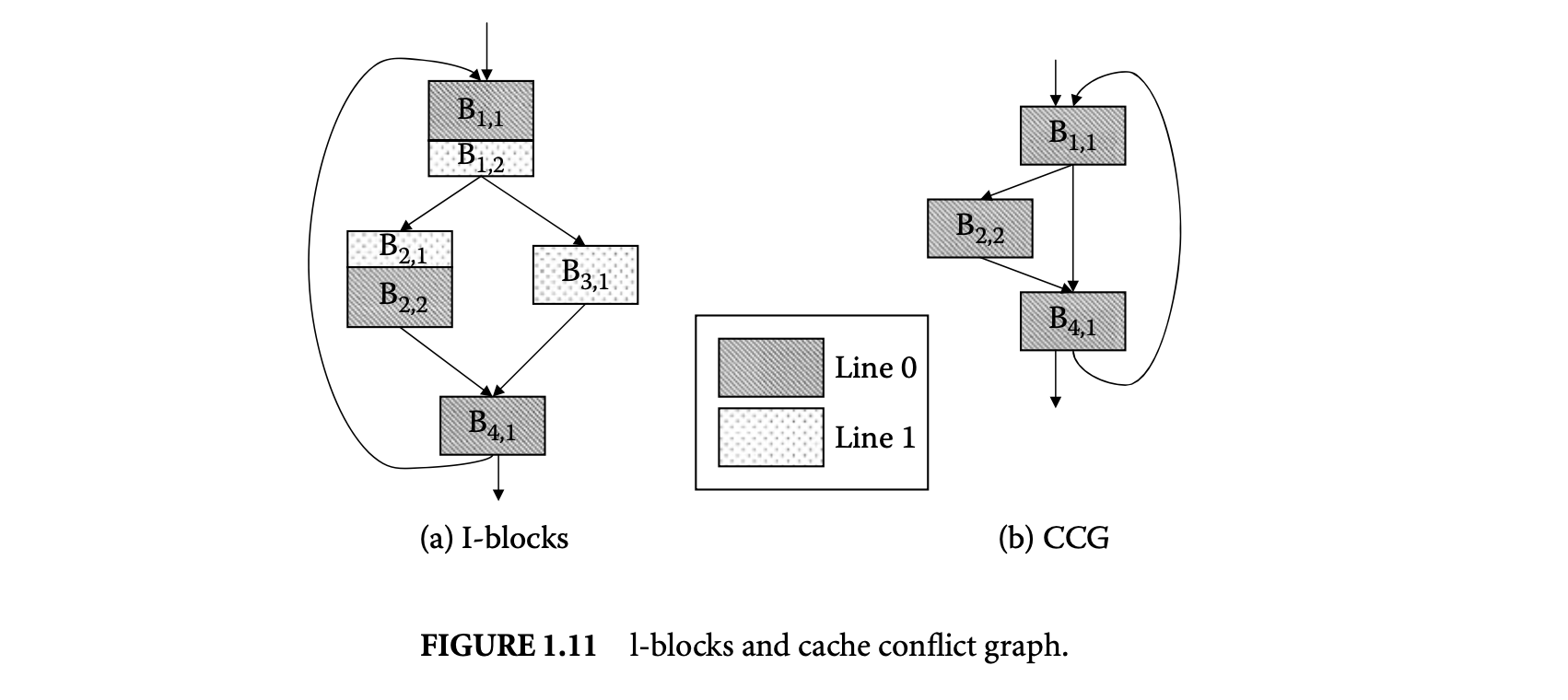
l-blocks mapped to cache line . An edge exists in if there exists a path in the control flow graph such that control flows from to , without going through any other l-block mapped to . In other words, there is an edge between l-blocks to if can be present in the cache when control reaches . Figure 11b shows the cache conflict graph corresponding to cache line for the control flow graph in Figure 11a mapped to a cache with two lines.
Let be the execution count of the edge between l-blocks and in a cache conflict graph. Now the execution count of l-block equals the execution count of basic block . Also, at each node of the cache conflict graph, the inflow equals the outflow and both equal the execution count of the node. Therefore,

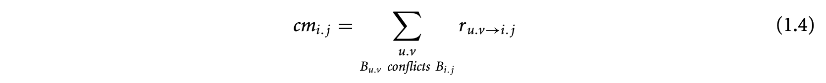
The cache miss count equals the inflow from conflicting l-blocks in the cache conflict graph. Any two1-blocks mapped to the same cache block are conflicting if they have different address tags. Two1-blocks mapped to the same cache block do not conflict when the basic block boundary is not aligned with the cache block boundary. For example, l-blocks and in Figure 11a occupy partial cache blocks and have the same address tags. They do not conflict with each other. Thus, we have
1.3.4.2 Dynamic Branch Prediction Modeling
Modern processors employ branch prediction to avoid performance loss due to control dependency [33]. Branch prediction schemes can be broadly categorized as static and dynamic. In the static scheme, a branch is predicted in the same direction every time it is executed. Though simple, static schemes are much less accurate than dynamic schemes.
1.3.4.2.1 Branch Terminology
Dynamic schemes predict a branch depending on the execution history. They use a entry branch prediction table to store past branch outcomes. When the processor encounters a conditional branch instruction, this prediction table is looked up using some index, and the indexed entry is used as prediction. When the branch is resolved, the entry is updated with the actual outcome. In practice, two-bit saturating counters are often used for prediction.
Different branch prediction schemes differ in how they compute an -bit index to access this table. In case of simplest prediction scheme, the index is lower-order bits of the branch address. More complex schemes use a single shift register called a branch history register (BHR) to record the outcomes of the most recent branches called history . The prediction table is looked up either using the BHR directly or exclusive or (XOR)-ed with the branch address. Considering the outcome of the neighboring branches exploits the correlation among consecutive branch outcomes.
Engblom [19] investigated the impact of dynamic branch prediction on the predicability of real-time systems. His experiments on a number of commercial processors indicate that dynamic branch prediction leads to high degree of execution time variation even for simple loops. In some cases, executing more iterations of a loop takes less time than executing fewer iterations. These results reaffirm the need to model branch prediction for WCET analysis.
1.3.4.2.2 Modeling
Li et al. [45] model dynamic branch predictors through ILP. The modeling is quite general and can be parameterized with respect to various prediction schemes. Modeling of dynamic branch prediction is somewhat similar to cache modeling. This is because they both use arrays (branch prediction table and cache) to maintain information. However, two crucial differences make branch prediction modeling significantly harder. First, a given branch instruction may use different entries of the prediction table at different points of execution (depending on the outcome of previous branches). However, an l-block always maps to the same cache block. Second, the flow of control between two conflicting l-blocks always implies a cache miss, but the flow of control between two branch instructions mapped to the same entry in the prediction table may lead to correct or incorrect prediction depending on the outcome of the two branches.
To model branch prediction, the objective function given in Equation 1.2 is modified to the following:

where is a constant denoting the penalty for a single branch misprediction, and is the number of times the branch in is mispredicted. The constraints now need to bound feasible values of . For simplicity, let us assume that the branch prediction table is looked up using the history as the index.
First, a terminating least-fixed-point analysis on the control flow graph identifies the possible values of history for each conditional branch. The flow constraints model the change in history along the control flow graph and thereby derive the upper bound on -- the execution count of the conditional branch at the end of basic block with history . Next, a structure similar to a cache conflict graph is used to bound the quantity denoting the number of times control flows from to such that the th entry of the prediction table is used for branch prediction at and and is never accessed in between. Finally, the constraints on the number of mispredictions are derived by observing the branch outcomes for consecutive accesses to the same prediction table entry as defined by .
1.3.4.3 Interaction between Cache and Branch Prediction
Cache and branch prediction cannot be modeled individually because of the wrong-path instruction prefetching effect (see Figure 1.10). An integrated modeling of these two components through ILP to capture the interaction has been proposed in [45]. First, the objective function is modified to include the timing effect of cache misses as well as branch prediction.
If we assume that the processor allows only one unresolved branch at any time during execution, then the number of branch mispredictions is not affected by instruction cache. However, the values of the number of cache misses may change because of the instruction fetches along the mispredicted path. The timing effects due to these additional instruction fetches can be categorized as follows:
- An l-block misses during normal execution since it is displaced by another conflicting l-block during speculative execution (destructive effect).
- An l-block hits during normal execution, since it is prefetched during speculative execution (constructive effect).
- A pending cache miss of during speculative execution along the wrong path causes the processor to stall when the branch is resolved. How long the stall lasts depends on the portion of cache miss penalty that is masked by the branch misprediction penalty. If the speculative fetching is completely masked by the branch penalty, then there is no delay incurred.
Both the constructive and destructive effects of branch prediction on cache are modeled by modifying the cache conflict graph. The modification adds nodes to the cache conflict graph corresponding to the l-blocks fetched along the mispredicted path. Edges are added among the additional nodes as well as between the additional nodes and the normal nodes depending on the control flow during misprediction. The third factor (delay due to incomplete cache miss when the branch is resolved) is taken care of by introducing an additional delay term in Equation 1.6.
1.3.4.4 Data Cache and Pipeline
So far we have discussed instruction cache and branch prediction modeling using ILP. Data caches are harder to model than instruction caches, as the exact memory addresses accessed by load/store instructions may not be known. A simulation-based analysis technique for data caches has been proposed in [50]. A program is broken into smaller fragments where each fragment has only one execution path. For example, even though there are many possible execution paths in a JPEG decompression algorithm, the execution paths of each computational kernel such as inverse discrete cosine transform (DCT), color transformation, and so on are simple. Each code fragment can therefore be simulated to determine the number of data cache hits and misses. These numbers can be plugged into the ILP framework to estimate the WCET of the whole program. For the processor pipeline, [50] again simulates the execution of a basic block starting with an empty pipeline state. The pipeline state at the end of execution of a basic block is matched against the instructions in subsequent basic blocks to determine the additional pipeline stalls during the overlap. These pipeline stalls are added up to the execution time of the basic block. It should be obvious that this style of modeling for data cache and pipeline may lead to underestimation in the presence of a timing anomaly.
Finally, Ottosson and Sjodin [60] propose a constraint-based WCET estimation technique that extends the ILP-based modeling. This technique takes the context, that is, the history, of execution into account. Each edge in the control flow graph now corresponds to multiple variables each representing a particular program path. This allows accurate representation of the state of the cache and pipeline before a basic block is executed. A constraint-based modeling propagates the cache states across basic blocks.
1.3.5 Integrated Approach Based on Timing Schema
As mentioned in Section 2, one of the original works on software timing analysis was based on timing schema [73]. In the original work, each node of the syntax tree is associated with a simple time bound. This simple timing information is not sufficient to accurately model the timing variations due to pipeline hazards, caches, and branch prediction. The timing schema approach has been extended to model a pipeline, instruction cache, and data cache in [51].
1.3.5.1 Pipeline Modeling
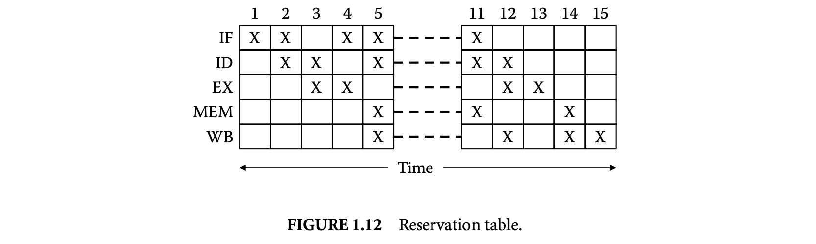
The execution time of a program construct depends on the preceding and succeeding instructions on a pipelined processor. A single time bound cannot model this timing variation. Instead a set of reservation tables associated with each program construct represents the timing information corresponding to different execution paths. A pruning strategy is used to eliminate the execution paths (and their corresponding reservation tables) that can never become the worst-case execution path of the program construct. The remaining set of reservation tables is called the worst-case timing abstraction (WCTA) of the program construct.
The reservation table represents the state of the pipeline at the beginning and end of execution of the program construct. This helps analyze the pipelined execution overlap among consecutive program constructs. The rows of the reservation table represent the pipeline stages and the columns represent time. Each entry in the reservation table specifies whether the corresponding pipeline stage is in use at the given time slot. The execution time of a reservation table is equal to its number of columns. Figure 12 shows a reservation table corresponding to a simple five-stage pipeline.
The rules corresponding to the sequence of statements and if-then-else and while-loop constructs can be extended as follows. The rule for a sequence of statements S: S1; S2 is given by

where W(S), W(S1), and W(S2) are the WCTAs of S, S1, and S2, respectively. The operator is defined as

[W_{1}\oplus W_{2}={w_{1}\oplus w_{2}|w_{1}\in W_{1},w_{2}\in W_{2}}]where and are reservation tables, and represents the concatenation of two reservation tables following the pipelined execution model. Similarly, the timing schema rule for S: if (exp) then S1 else S2 is given by

where is the set union operation. Finally, the rule for the construct S: while (exp) S1 is given by

where N is the loop bound. In all the cases, a reservation table can be eliminated from the WCTA if it can be guaranteed that w will never lead to the WCET of the program. For example, if the worst-case scenario (zero overlap with neighboring instructions) involving is shorter than the best-case scenario (complete overlap with neighboring instructions) involving , then can be safely eliminated from .
1.3.5.2 Instruction Cache Modeling
To model the instruction cache, the WCTA is extended to maintain the cache state information for a program construct. The main observation is that some of the memory accesses can be resolved locally (within the program construct) as cache hit/miss. Each reservation table should therefore include (a) the first reference to each cache block as its hit or miss depends on the cache content prior to the program construct (first_reference) and (b) the last reference to each cache block (last_reference). The latter affects the timing of the successor program construct(s).
The timing rules are structurally identical to the pipeline modeling, but the semantics of the operator is modified. Let us assume a direct-mapped instruction cache. Then inherits for a cache block the first_reference of except when does not have any access to . In that case, inherits the first_reference of . Similarly, for a cache block , inherits the last_reference of except when does not have a last_reference to . In this case, the last_reference to is inherited from . Finally, the number of additional cache hits for can be determined by comparing the first_references of with the last_references of . The execution time of can be determined by taking into account the pipelined execution across and the additional cache hits. As before, a pruning strategy is employed to safely eliminate WCTA elements that can never contribute to the WCET path of the program.
1.3.5.3 Data Cache Modeling
Timing analysis of the data cache is similar to that of the instruction cache. The major difficulty, however, is that the addresses of some data references may not be known at compile time. A global data flow analysis [38] is employed to resolve the data references of load/store instructions as much as possible. A conservative approach is then proposed [38] where two cache miss penalties are assumed for each data reference whose memory address cannot be determined at compile time. The data reference is then ignored in the rest of the analysis. The first penalty accounts for the cache miss possibility of the data reference. The second penalty covers for the possibility that the data reference may replace some memory block (from the cache) that is considered as cache hit in the analysis. Finally, data dependence analysis is utilized to minimize the WCET overestimation resulting from the conservative assumption of two cache misses per unknown reference.
1.3.6 Separated Approach Based on Abstract Interpretation
ILP-based WCET analysis methods can model the architectural components and their interaction in an accurate fashion, thereby yielding tight estimates. However, ILP solution time may increase considerably with complex architectural features. To circumvent this problem, Theiling et al. [82] have proposed a separated approach where abstract interpretation is employed for micro-architectural modeling followed by ILP for path analysis. As there is a dependency between the two steps, micro-architectural modeling has to produce conservative estimates to ensure safety of the result. This overestimation is offset by significantly faster analysis time.
Abstract interpretation [15] is a theory for formally constructing conservative approximations of the semantics of a programming language. A concrete application of abstract interpretation is in static program analysis where a program's computations are performed using abstract values in place of concrete values. Abstract interpretation is used in WCET analysis to approximate the "collecting semantics" at a program point. The collecting semantics gives the set of all program states (cache, pipeline, etc.) for a given program point. In general, the collecting semantics is not computable. In abstract interpretation, the goal is to produce an abstract semantics which is less precise but effectively computable. The computation of the abstract semantics involves solving a system of recursive equations/constraints. Given a program, we can associate a variable to denote the abstract semantics at program point . Clearly, will depend on the abstract semantics of program points preceding . Since programs have loops, this will lead to a system of recursive constraints. The system of recursive constraints can be iteratively solved via fixed-point computation. Termination of the fixed-point computation is guaranteed only if (a) the domain of abstract values (which is used to define the abstract program semantics) is free from infinite ascending chains and (b) the iterative estimates of grow monotonically. The latter is ensured if the semantic functions in the abstract domain, which show the effect of the programming language constructs in the abstract domain and are used to iteratively estimate , are monotonic.
Once the fixed-point computation terminates, for every program point , we obtain a stable estimate for -- the abstract semantics at . This is an overapproximation of all the concrete states with which could be reached in program executions. Thus, for cache behavior modeling, could be used to denote an overapproximation of the set of concrete cache states with which program point could be reached in program executions. This abstract semantics is then used to conservatively derive the WCET bounds for the individual basic blocks. Finally, the WCET estimates of basic blocks are combined with ILP-based path analysis to estimate the WCET of the entire program.
1.3.6.1 Cache Modeling
To illustrate AI-based cache modeling, we will assume a fully associative cache with a set of cache lines and least recently used replacement policy. Let denote the set of memory blocks. The absence of any memory block in a cache line is indicated by a new element ; thus, .
Let us first define the concrete semantics.
Definition 1.3: A concrete cache state is a function .
If for a concrete cache state , then there are elements that are more recently used than . In other words, is the relative age of . denotes the set of all concrete cache states.
Definition 1.4: A cache update function describes the new cache state for a given cache state and a referenced memory block.
Let be the referenced memory block. The cache update function shifts the memory blocks , which have been more recently used than , by one position to the next cache line. If was not in the cache, then all the memory blocks are shifted by one position, and the least recently used memory block is evicted from the cache state (if the cache was full). Finally, the update function puts the referenced memory block in the first position .
The abstract semantics defines the abstract cache states, the abstract cache update function, and the join function.
Definition 1.5: An abstract cache state maps cache lines to sets of memory blocks.
Let denote the set of all abstract cache states. The abstract cache update function is a straightforward extension of the function (which works on concrete cache states) to abstract cache states.
Furthermore, at control flow merge points, join functions are used to combined the abstract cache states. That is, join functions approximate the collecting semantics depending on program analysis.
Definition 1.6: A join function combines two abstract cache states.
Since is finite and is finite, clearly the domain of abstract cache states is finite and hence free from any infinite ascending chains. Furthermore, the update and join functions and are monotonic. This ensures termination of a fixed-point computation-based analysis over the above-mentioned abstract domain. We now discuss two such analysis methods.
The program analysis mainly consists of must analysis and may analysis. The must analysis determines the set of memory blocks that are always in the cache at a given program point. The may analysis determines the memory blocks that may be in the cache at a given program point. The may analysis can be used to determine the memory blocks that are guaranteed to be absent in the cache at a given program point.
The must analysis uses abstract cache states with upper bounds on the ages of the memory blocks in the concrete cache states. That is, if , then is guaranteed to be in the cache for at least the next memory references ( is the number of cache lines). Therefore, the join function of two abstract cache states and puts a memory block in the new cache state if and only if is present in both and . The new age of is the maximum of its ages in and . Figure 1.13 shows an example of the join function for must and may analysis.
The may analysis uses abstract cache states with lower bounds on the ages of the memory blocks. Therefore, the join function of two abstract cache states and puts a memory block in the new cache state if is present in either or or both. The new age of is the minimum of its ages in and .
At a program point, if a memory block is present in the abstract cache state after must analysis, then a memory reference to will result in a cache hit (always hit). Similarly, if a memory block is absent in the abstract cache state after may analysis, then a memory reference to will result in a cache miss (always miss). The other memory references cannot be classified as hit or miss. To improve the accuracy, a further persistence analysis can identify memory blocks for which the first reference may result in either hit or miss, but the remaining references will be hits.
These categorization of memory references is used to define the WCET for each basic block. To improve the accuracy, the WCET of a basic block is determined under different calling contexts. Thus, the objective
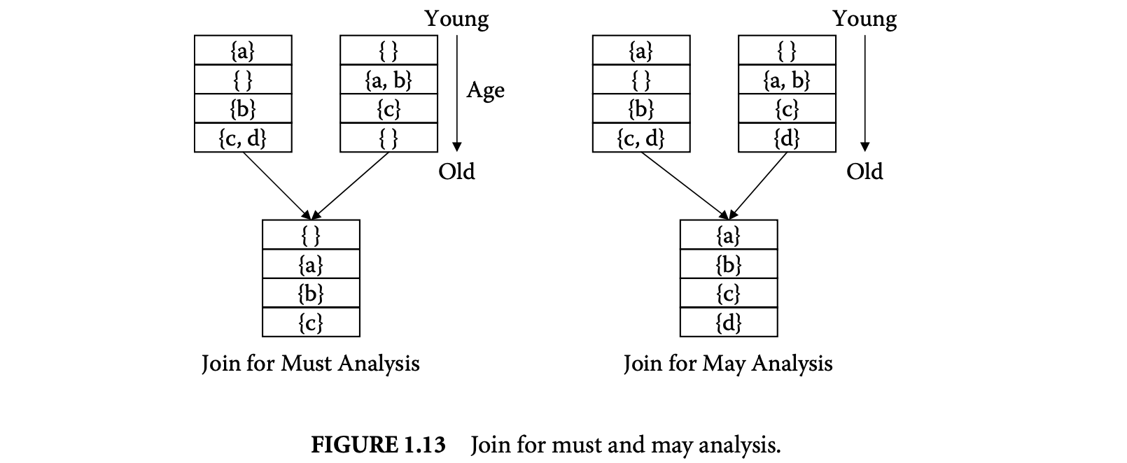
function can be defined as

where denotes the set of all calling contexts for basic block . The bounds on execution counts can be derived by ILP-based path analysis.
An extension for data cache modeling using abstract interpretation has been proposed in [23]. The basic idea is to extend the cache update function such that it can handle cases where not all addresses referenced by a basic block are known.
Another technique for categorizing cache access references into always hit, always miss, first miss, and first hit has been proposed by the group at Florida State University [4, 57, 93]. They perform categorization through static cache simulation, which is essentially an interprocedural data flow analysis. This categorization is subsequently used during pipeline analysis [29]. Pipeline analysis proceeds by determining the total number of cycles required to execute each path, where a path consists of all the instructions that can be executed during a single iteration of a loop. The data hazards and the structural hazards across paths are determined by maintaining the first and last use of each pipeline stage and register within a path. As mentioned before, this separation of cache analysis from the pipeline analysis may not be safe in the presence of a timing anomaly.
1.3.6.2 Pipeline Modeling
To model a pipeline with abstract interpretation [41], concrete execution on a concrete pipeline can be viewed as applying a function. This function takes as input a concrete pipeline state and a sequence of instructions in a basic block . It produces a sequence of execution states, called a trace, and a final concrete state when executing . The length of the trace determines the number of cycles the execution takes. The concept of trace is similar to the reservation table described in the context of timing-schema-based analysis.
However, in the presence of incomplete information, such as nonclassified cache accesses, the concrete execution is not feasible. Therefore, pipeline analysis employs an abstract execution of the sequence of instructions in a basic block starting with an abstract pipeline state [41]. This modeling defines an abstract pipeline state as a set of concrete pipeline states, and pipeline states with identical timing behavior are grouped together. Now, suppose that in an abstract pipeline state an event occurs that changes the pipeline states, such as the issue/execution of an instruction in a basic block. If the latency of this event can be statically determined, has only one successor state. However, if the latency of 's execution cannot be statically determined, a pipeline state will have several successor states resulting from the execution of corresponding to the various possible latencies of (thereby causing state space explosion). In this way, reachable pipeline states within a basic block will be enumerated (while grouping together states with identical timing behavior) in order to determine the basic block's WCET.
For a processor without a timing anomaly [41], the abstract execution can be employed to each basic block starting with the empty pipeline state. The abstract execution exploits the memory reference categorization (obtained through cache modeling) to determine memory access delays during pipeline execution. Therefore, abstract execution of a basic block should happen under different contexts. In the presence of a timing anomaly, cache and pipeline analysis cannot be separated [32]. Hence the abstract states now consist of pairs of abstract pipeline states and abstract cache states. Moreover, the final abstract states of a basic block will be passed on to the successor basic block(s) as initial states. Clearly, this can lead to an exponential number of abstract states for complex processor pipelines.
1.3.6.3 Branch Prediction Modeling
Colin and Puaut [14] propose abstract-interpretation-based branch prediction modeling. They assume that the branch prediction table (see Section 1.3.4.2.1) is indexed using the address of the conditional branch instruction. This prediction scheme is simpler and hence easier to model than the BHR-based predictors modeled using ILP [45]. Colin and Puaut use the term branch target buffer (BTB) instead of prediction table, as it stores the target address in addition to the branch history. Moreover, each entry in the BTB is tagged with the address of the conditional branch instruction whose history and target address are stored in that entry. When a conditional branch is encountered, if its address is in the BTB, then it is predicted based on the history stored in the BTB. Otherwise, the default prediction of the branch not taken is used. The BTB is quite similar to instruction cache and indeed can be organized as direct-mapped or s-way set associative caches.
The abstract execution defines the abstract buffer state (ABS) corresponding to the BTB. Each basic block is associated with two ABS: and , representing the BTB state before and after 's execution. An ABS indicates for each BTB entry which conditional branch instructions can be in the BTB at that time. At program merge points, a set union operation is carried out. Thus,

where is the set of basic blocks preceding in the control flow graph. Assuming a set-associative BTB, the union operator is defined as follows:

where is a set containing all the branch instructions that could be in the th entry of the set . is derived from by taking into account the conditional branch instruction in .
Given , the conditional branch instruction can be classified as history predicted if it is present in the BTB and default predicted otherwise. However, a history-predicted instruction does not necessarily lead to correct prediction. Similarly, a default-predicted instruction does not always lead to misprediction. This is taken into account by considering the behavior of the conditional branch instruction. For example, a history-predicted loop instruction is always correctly predicted except for loop exit.
The modeling in [14] was later extended to more complex branch predictors such as bimodal and global-history branch prediction schemes [5, 11]. The semantic context of a branch instruction in the source code is taken into account to classify a branch as easy to predict or hard to predict. Easy-to-predict branches are analyzed, while conservative misprediction penalties are assumed for hard-to-predict branches. The downside of these techniques is that they make a restrictive assumption of each branch instruction mapping to a different branch table entry (i.e., no aliasing).
1.3.7 A Separated Approach That Avoids State Enumeration
The implication of a timing anomaly (see Section 1.3.2) is that all possible schedules of instructions have to be considered to estimate the WCET of even a basic block. Moreover, all possible processor states at the end of the preceding and succeeding basic blocks have to be considered during the analysis of a basic block. This can result in state space explosion for analysis techniques, such as abstract-interpretation-based modeling, that are fairly efficient otherwise [83].
A novel modeling technique [46] obtains safe and tight estimates for processors with timing anomalies without enumerating all possible executions corresponding to variable latency instructions (owing to cache miss, branch misprediction, and variable latency functional units). In particular, [46] models a fairly complex out-of-order superscalar pipeline with instruction cache and branch prediction. First, the problem is formulated as an execution graph capturing data dependencies, resource contentions, and degree of superscalarity -- the major factors dictating instruction executions. Next, based on the execution graph, the estimation algorithm starts with very coarse yet safe timing estimates for each node of the execution graph and iteratively refines the estimates until a fixed point is reached.
1.3.7.1 Execution Graph
Figure 1.14 shows an example of an execution graph. This graph is constructed from a basic block with five instructions as shown in Figure 1.14a; we assume that the degree of superscalarity is 2. The processor has five pipeline stages: fetch (IF), decode (ID), execute (EX), write back (WB), and commit (CM). A decoded instruction is stored in the re-order buffer. It is issued (possibly out of order) to the corresponding functional unit for execution when the operands are ready and the functional unit is available.
Let represent the sequence of instructions in a basic block . Then each node in the corresponding execution graph is represented by a tuple: an instruction identifier and a pipeline stage denoted as stage(instruction_id). For example, the node represents the fetch stage of the instruction . Each node in the execution graph is associated with the latency of the corresponding pipeline stage. For a node with variable latency , the node is annotated with an interval . As some resources (e.g., floating point multiplier) in modern processors are fully pipelined, such resources are annotated with initiation intervals. The initiation interval of a resource is defined as the number of cycles that must elapse between issuing two instructions to that resource. For example, a fully pipelined floating point multiplier can have a latency of six clock cycles and an initiation interval of one clock cycle. For a nonpipelined resource, the initiation interval is the same as latency. Also, if there exist multiple copies of the same resource (e.g., two arithmetic logical units (ALUs)), then one needs to define the multiplicity of that resource.
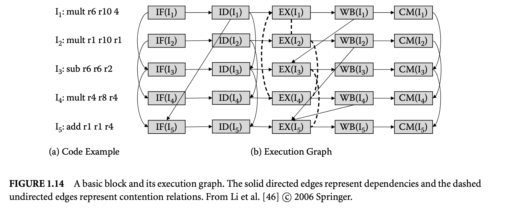
The dependence relation from node to node in the execution graph denotes that can start execution only after has completed execution; this is indicated by a solid directed edge from to in the execution graph. The analysis models the following dependencies:
- Dependencies among pipeline stages of the same instruction.
- Dependencies due to finite-sized buffers and queues such as I-buffer or ROB. For example, assuming a four-entry I-buffer, there will be no entry available for before the completion of (which removes from the I-buffer). Therefore, there should be a dependence edge .
- Dependencies due to in-order execution in IF, ID, and CM pipeline stages. For example, in a scalar processor (i.e., degree of ) there will be dependence edges because can only start after completes. For a superscalar processor with -way fetch (i.e., degree of ), there are dependence edges . This captures the fact that cannot be fetched in the same cycle as .
- Data dependencies among instructions. If instruction produces a result that is used by instruction , then there should be a dependence edge .
Apart from the dependence relation among the nodes in an execution graph (denoted by solid edges), there also exist contention relations among the execution graph nodes. Contention relations model structural hazards in the pipeline. A contention relation exists between two nodes and if they can delay each other by contending for a resource, for example, functional unit or register write port. The contention between and is shown as an undirected dashed edge in the execution graph. A contention relation makes it possible for an instruction later in the program order to delay the execution of an earlier instruction.
Finally, a parallelism relation is defined to model superscalarity, for example, multiple issues and multiple decodes. Two nodes and participate in a parallelism relation iff (a) nodes and denote the same pipeline stage (call it ) of two different instructions and and (b) instructions and can start execution of this pipeline stage in parallel.
1.3.7.2 Problem Definition
Let be a basic block consisting of a sequence of instructions . Estimating the WCET of can be formulated as finding the maximum (latest) completion time of the node , assuming that starts at time zero. Note that this problem is not equivalent to finding the longest path from to in 's execution graph (taking the maximum latency of each pipeline stage). The execution time of a path in the execution graph is not a summation of the latencies of the individual nodes for two reasons:
- The total time spent in making the transition from to is dependent on the contentions from other ready instructions.
- The initiation time of a node is computed as the max of the completion times of its immediate predecessors in the execution graph. This models the effect of dependencies, including data dependencies.
1.3.7.3 Estimation Algorithm
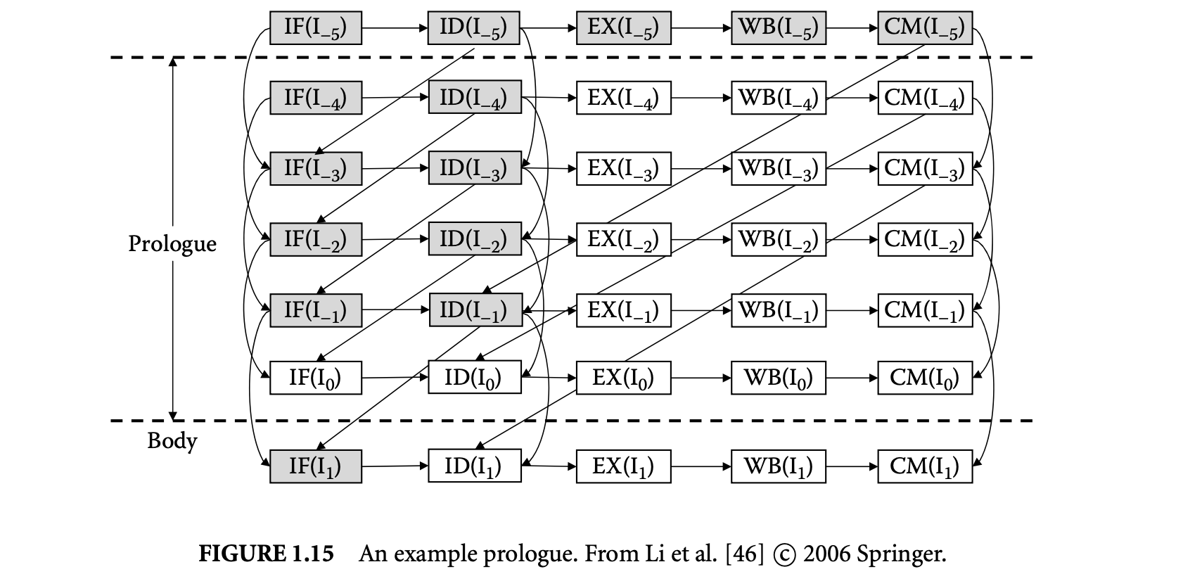
The timing effects of the dependencies are accounted for by using a modified longest-path algorithm that traverses the nodes in topologically sorted order. This topological traversal ensures that when a node is visited, the completion times of all its predecessors are known. To model the effect of resource contentions, the algorithms conservatively estimate an upper bound on the delay due to contentions for a functional unit by other instructions. A single pass of the modified longest-path algorithm computes loose bounds on the lifetime of each node. These bounds are used to identify nodes with disjoint lifetimes. Thesenodes are not allowed to contend in the next pass of the longest-path search to get tighter bounds. These two steps repeat until there is no change in the bounds. Termination is guaranteed for the following reasons:
- The algorithm starts with all pairs of instructions in the contention relation (i.e., every instruction can delay every other instruction).
- At every step of the fixed-point computation, pairs are removed from this set -- those instruction pairs that are shown to be separated in time.
As the number of instructions in a basic block is finite, the number of pairs initially in the contention relation is also finite. Furthermore, the algorithm removes at least one pair in every step of the fixed-point computation, so the fixed-point computation must terminate in finitely many iterations; if the number of instructions in the basic block being estimated is , the number of fixed-point iterations is bounded by .
1.3.7.3.1 Basic Block Context
In the presence of a timing anomaly, a basic block cannot be analyzed in isolation by assuming an empty pipeline at the beginning. The instructions before (after) a basic block that directly affect the execution time of constitute the contexts of and are called the prologue (epilogue) of . As processor buffer sizes are finite, the prologue and epilogue contain finite number of instructions. Of course, a basic block may have multiple prologues and epilogues corresponding to the different paths along which can be entered or exited. To capture the effects of contexts, the analysis technique constructs execution graphs corresponding to all possible combinations of prologues and epilogues. Each execution graph consists of three parts: the prologue, the basic block itself (called the body), and the epilogue.
The executions of two or more successive basic blocks have some overlap due to pipelined execution. The overlap between a basic block and its preceding basic block is the period during which instructions from both the basic blocks are in the pipeline, that is,

where is the last instruction of block (predecessor) and is the first instruction of block . To avoid duplicating the overlap in time estimates of successive basic blocks, the execution time of a basic block is defined as the interval from the time when the instruction immediately preceding has finished committing to the time when 's last instruction has finished committing, that is,

where is the instruction immediately prior to and is the last instruction of .
The execution time for basic block is estimated with respect to (w.r.t.) the time at which the first instruction of is fetched, i.e., . Thus, can be conservatively estimated by finding the largest value of and the smallest value of .

1.3.7.3.2 Overall Pipeline Analysis
The execution time estimate of a basic block is obtained for a specific prologue and a specific epilogue of . A basic block in general has multiple choices of prologues and epilogues. Thus, 's execution time is estimated under all possible combinations of prologues and epilogues. The maximum of these estimates is used as 's WCET . Let and be the set of prologues and epilogues for .

is used in defining the WCET of the program as the following objective function:

The quantity denotes the execution count of basic block and is a variable. is the set of all basic blocks in the program. This objective function is maximized over the constraints on given by ILP-based path analysis.
1.3.7.4 Integrating Cache and Branch Prediction Analysis
The basic idea is to define different scenarios for a basic block corresponding to cache miss and branch misprediction. If these scenarios are defined suitably, then we can estimate a constant that bounds the execution time of a basic block corresponding to each scenario. Finally, the execution frequencies of these scenarios are defined as ILP variables and are bounded by additional linear constraints.
Scenarios corresponding to cache misses are defined as follows. Given a cache configuration, a basic block can be partitioned into a fixed number of memory blocks, with instructions in each memory block being mapped to the same cache block (cache accesses of instructions other than the first one in a memory block are always hits). A cache scenario of is defined as a mapping of hit or miss to each of the memory blocks of . The memory blocks are categorized into always hit, always miss, or unknown, using abstract interpretation-based modeling (see Section 1.3.6.1). The upper bounds on the execution time of are computed w.r.t. each of the possible cache scenarios. For the first instructions in memory blocks with unknown categorization, the latency of the fetch stage is assumed to be where is the cache miss penalty.
Similarly, the scenarios for branch prediction are defined as the two branch outcomes (correct prediction and misprediction) corresponding to each of the predecessor basic blocks. The execution time of the basic block is estimated w.r.t. both the scenarios by adding nodes corresponding to the wrong-path instructions to the execution graph of a basic block.
Considering the possible cache scenarios and correct or wrong prediction of the preceding branch for a basic block, the ILP objective function denoting a program's WCET is now written as follows.

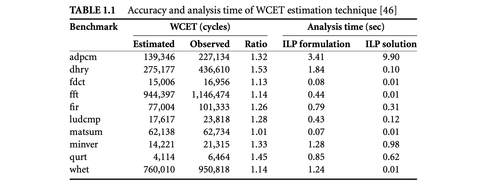
where is the WCET of executed under the following context: (a) is reached from a preceding block , (b) the branch prediction at the end of is correct or does not have a conditional branch, and (c) is executed under a cache scenario . is the set of all cache scenarios of block . The bounds on number of scenarios with correct and mispredicted branch instructions are obtained using ILP-based analysis [45] (see Section 1.3.4.2).
Finally, to extend the above approach for modeling data caches, one can adapt the approach of [69]. This work augments the cache miss equation framework of Ghosh et al. [26] to generate accurate hit and miss patterns corresponding to memory references at different loop levels.
1.3.7.5 Accuracy and Scalability
To give the readers a feel of the accuracy and scalability of the WCET analysis techniques, we present in Table 1.1 the experimental results from [46]. The processor configuration used here is fairly sophisticated: a 2-way superscalar out-of-order pipeline with 5 stages containing a 4-entry instruction fetch buffer, an 8-entry re-order buffer, 2 ALUs, variable latency multiplication and floating point units, and 1 load/store unit; perfect data cache; gshare branch predictor with a 128-entry branch history table; a 1-KB 2-way set associative instruction cache with 16 sets, 32 bytes line size, and 30 cycles cache miss penalty. The analysis was run on a 3-GHz Pentium IV PC with 2 GB main memory.
Table 1.1 presents the estimated WCET obtained through static analysis and the observed WCET obtained via simulation (see Figure 1.3 for the terminology). The estimated WCET is quite close to the observed WCET. Also, the total estimation time (ILP formulation + ILP solving) is less than 15 seconds for all the benchmarks.
1.4 Worst-Case Energy Estimation
In this section, we present a static analysis technique to estimate safe and tight bounds for the worst-case energy consumption of a program on a particular processor. The presentation in this section is based on [36].
Traditional power simulators, such as Wattch [9] and SimplePower [96], perform cycle-by-cycle power estimation and then add them up to obtain total energy consumption. Clearly, we cannot use cycle-accurate estimation to compute the worst-case energy bound, as it would essentially require us to simulate all possible scenarios (which is too expensive). The other method [75, 88] is to use fixed per-instruction energy but it fails to capture the effects of cache miss and branch prediction. Instead, worst-case energy analysis is based on the key observation that the energy consumption of a program can be separated out into the following time-dependent and time-independent components:
Instruction-specific energy: The energy that can be attributed to a particular instruction (e.g., energy consumed as a result of the execution of the instruction in the ALU, cache miss, etc.). Instruction-specific energy does not have any relation with the execution time. Pipeline-specific energy: The energy consumed in the various hardware components (clock network power, leakage power, switch-off power, etc.) that cannot be attributed to any particular instruction. Pipeline-specific energy is roughly proportional to the execution time.
Thus, cycle-accurate simulation is avoided by estimating the two energy components separately. Pipeline-specific energy estimation can exploit the knowledge of WCET. However, switch-off power and clock network power make the energy analysis much more involved -- we cannot simply multiply the WCET by a constant power factor. Moreover, cache misses and overlap among basic blocks due to pipelining and branch prediction add significant complexity to the analysis.
1.4.1 Background
Power and energy are terms that are often used interchangeably as long as the context is clear. For battery life, however, the important metric is energy rather than power. The energy consumption of a task running on a processor is defined as , where is the average power and is the execution time. Energy is measured in Joules, whereas power is measured in Watts (Joules/second). Power consumption consists of two main components: dynamic power and leakage power .
Dynamic power is caused by the charging and discharging of the capacitive load on each gate's output due to switching activity. It is defined as , where is the switching activity, is the supply voltage, is the capacitance, and is the clock frequency. For a given processor architecture, and are constants. The capacitance value for each component of the processor can be derived through register-capacitor (RC)-equivalent circuit modeling [9].
Switching activity is dependent on the particular program being executed. For circuits that charge and discharge every cycle, such as double-ended array bitlines, an activity factor of 1.0 can be used. However, for other circuits (e.g., single-ended bitlines, internal cells of decoders, pipeline latches, etc.), an accurate estimation of the activity factor requires examination of the actual data values. It is difficult, if not impossible, to estimate the activity factors through static analysis. Therefore, an activity factor of 1.0 (i.e., maximum switching) is assumed conservatively for each active processor component.
Modern processors employ clock gating to save power. This involves switching off clock signals to the idle components so they do not consume dynamic power in the unused cycles. Jayaseelan et al. [36] model three different clock gating styles. For simplicity, let us assume a realistic gating style where idle units and ports dissipate 10% of the peak power. A multi-ported structure consumes power proportional to the number of ports accessed in a given cycle. The power consumed in the idle cycles is referred to as switch-off power.
A clock distribution network consumes a significant fraction of the total energy. Without clock gating, clock power is independent of the characteristics of the applications. However, clock gating results in power savings in the clock distribution network. Whenever the components in a portion of the chip are idle, the clock network in that portion of the chip can be disabled, reducing clock power.
Leakage power captures the power lost from the leakage current irrespective of switching activity. The analysis uses the leakage power model proposed in [98]: , where is the supply voltage and is the number of transistors. is a constant specifying the leakage current corresponding to a particular process technology. is an empirically determined design parameter obtained through SPICE simulation corresponding to a particular device.
1.4.2 Analysis Technique
The starting point of the analysis is the control flow graph of the program. The first step of the analysis estimates an upper bound on the energy consumption of each basic block. Once these bounds are known, the worst-case energy of the entire program can be estimated through path analysis.
1.4.2.1 Energy Estimation for a Basic Block
The goal here is to estimate a tight upper bound on the total energy consumption of a basic block through static analysis. From the discussion in Section 1.4.1,

where is the instruction-specific energy component, that is, the energy consumed as a result of switching activity as an instruction goes through the pipeline stages. , , and are defined as the energy consumed as a result of the switch-off power, leakage power, and clock power, respectively, during , where is the WCET of the basic block . The WCET () is estimated using the static analysis techniques. Now we describe how to define bounds for each energy component.
Dynamic EnergyThe instruction-specific energy of a basic block is the dynamic power consumed as a result of the switching activity generated by the instructions in that basic block.

where is the dynamic power consumed by an instruction . Now, let us analyze the energy consumed by an instruction as it travels through the pipeline:
- Fetch and decode: The energy consumed here is due to fetch, decode, and instruction cache access. This stage needs feedback from cache analysis.
- Register access: The energy consumed for the register file access because of reads/writes can vary from one class of instructions to another. The energy consumption in the register file for an instruction is proportional to the number of register operands.
- Branch prediction: The energy consumption in this stage needs feedback from branch prediction modeling.
- Wakeup logic: When an operation produces a result, the wakeup logic is responsible for making the dependent instructions ready, and the result is written onto the result bus. An instruction places the tag of the result on the wakeup logic and the actual result on the result bus exactly once, and the corresponding energy can be easily accounted for. The energy consumed in the wakeup logic is proportional to the number of output operands.
- Selection logic: Selection logic is interesting from the point of view of energy consumption. The selection logic is responsible for selecting an instruction to execute from a pool of ready instructions. Unlike the other components discussed earlier, an instruction may access the selection logic more than once. This is because an instruction can request a specific functional unit and the request might not be granted, in which case it makes a request in the next cycle. However, we cannot accurately determine the number of times an instruction would access the selection logic. Therefore, it is conservatively assumed that the selection logic is accessed every cycle.
- Functional units: The energy consumed by an instruction in the execution stage depends on the functional unit it uses and its latency. For variable latency instructions, one can safely assume the maximum energy consumption. The energy consumption for load/store units depends on data cache modeling.
Now, Equation 1.13, corresponding to dynamic energy consumed in a basic block , is redefined as
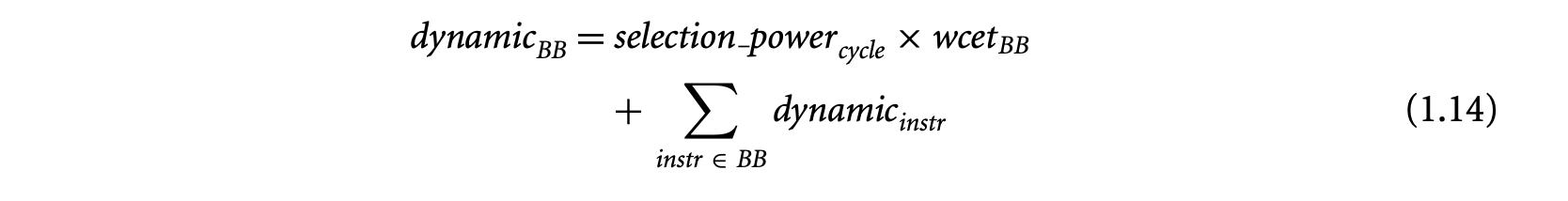
where is a constant defining the power consumed in the selection logic per cycle. is the WCET of BB. Note that is redefined as the power consumed by in all the pipeline stages except for selection logic.
As mentioned before, pipeline-specific energy consists of three components: switch-off energy, clock energy, and leakage energy. All three energy components are influenced by the execution time of the basic block.
Switch-off Energy
The switch-off energy refers to the power consumed in an idle unit when it is disabled through clock gating. Let be the total number of accesses to a component by the instructions in basic block BB. Let be the maximum number of allowed accesses/ports for component per cycle. Then, switch-off energy for component in basic block BB is
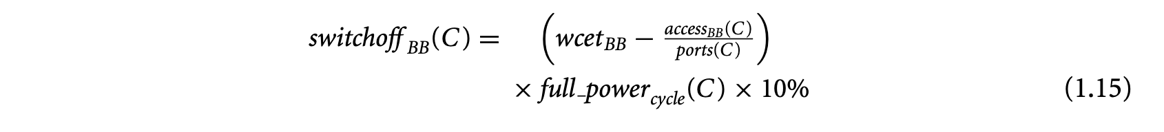
where is the full power consumption per cycle for component . The switch-off energy corresponding to a basic block can now be defined as

where components is the set of all hardware components.
1.4.2.1.3 Clock Network Energy
To estimate the energy consumed in the clock network, clock gating should be taken into account.

where is the clock energy without gating and can be defined as

where is the peak power consumed per cycle in the clock network. is defined as the power consumed in all the components except clock network in the presence of clock gating. That is,

, however, is the power consumed in all the components except clock network in the absence of clock gating. It is simply defined as

is a constant defining the peak dynamic plus leakage power per cycle excluding the clock network.
1.4.2.1.4 Leakage Energy
The leakage energy is simply defined as , where is the power lost per processor cycle from the leakage current regardless of the circuit activity. This quantity, as defined in Section 1.4.1, is a constant given a processor architecture. is, as usual, the WCET of BB.
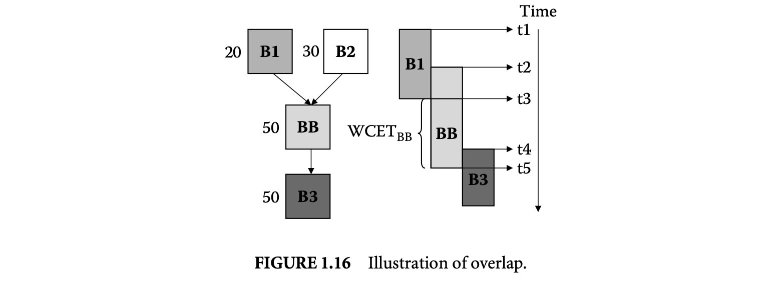
1.4.2.2 Estimation for the Whole Program
Given the energy bounds for the basic blocks, we can now estimate the worst-case energy consumption of a program using an ILP formulation. The ILP formulation is similar to the one originally proposed by Li and Malik [50] to estimate the WCET of a program. The execution times of the basic blocks are replaced with the corresponding energy consumptions. Let be the upper bound on the energy consumption of a basic block . Then the total energy consumption of the program is given by
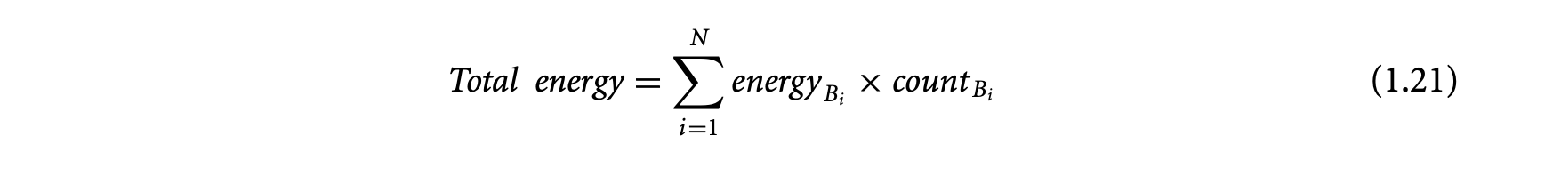
where the summation is taken over all the basic blocks in the program. The worst-case energy consumption of the program can be derived by maximizing the objective function under the flow constraints through an ILP solver.
1.4.2.3 Basic Block Context
A major difficulty in estimating the worst-case energy arises from the overlapped execution of basic blocks. Let us illustrate the problem with a simple example. Figure 1.16 shows a small portion of the control flow graph. Suppose we are interested in estimating the energy bound for basic block . The annotation for each basic block indicates the maximum execution count. This is just to show that the execution counts of overlapped basic blocks can be different. As the objective function (defined by Equation 1.21) multiplies each with its execution count , we cannot arbitrarily transfer energy between overlapping basic blocks. Clearly, instruction-specific energy of should be estimated based on only the energy consumption of its instructions. However, we cannot take such a simplistic view for pipeline-specific energy. Pipeline-specific energy depends critically on .
If we define without considering the overlap, that is, , then it results in excessive overestimation of the pipeline-specific energy values as the time intervals and are accounted for multiple times. To avoid this, we can redefine the execution time of as the time difference between the completion of execution of the predecessor ( in our example) and the completion of execution of , that is, . Of course, if has multiple predecessors, then we need to estimate for each predecessor and then take the maximum value among them.
This definition of execution time, however, cannot be used to estimate the pipeline-specific energy of in a straightforward fashion. This is because switch-off energy and thus clock network energy depend on the idle cycles for hardware ports/units. As we are looking for worst-case energy, we need to estimate an upper bound on idle cycles. Idle cycle estimation (see Equation 1.15) requires an estimate of , which is defined as the total number of accesses to a component by the instructions in basic block . Now, with the new definition of as the interval , not all these accesses fall within , and we run the risk of underestimating idle cycles. To avoid this problem, in Equation 1.15 is replaced with which is defined as the total number of accesses to a component C by the instructions in basic block BB that are guaranteed to occur within
 The number of accesses according to this new definition is estimated during the WCET analysis of a basic block. The energy estimation techniques use the execution-graph-based WCET analysis technique [46] discussed in Section 1.3.7. Let be the latest commit time of the last instruction of the predecessor node and be the earliest commit time of the last instruction of B B. Then, for each pipeline stage of the different instructions in B B, the algorithm checks whether its earliest or latest start time falls within the interval . If the answer is yes, then the accesses corresponding to that pipeline stage are guaranteed to occur within and are included in . The pipeline-specific energy is now estimated w.r.t. each of B B 's predecessors, and the maximum value is taken.
1.4.2.4 Integrating Cache and Branch Prediction Analysis
Integration of cache and branch prediction modeling is similar to the method described in the context of execution-graph-based WCET analysis (Section 1.3.7). For each cache scenario, the analysis adds the dynamic energy due to cache misses defined as

where is the main memory energy for BB corresponding to cache scenario , is the number of cache misses in BB corresponding to cache scenario , and is a constant defining the energy consumption per main memory access.
The additional instruction-specific energy due to the execution of speculative instructions is estimated as follows. Let be a basic block with as the predecessor (see Figure 1.17). If there is a misprediction for the control flow , then instructions along the basic block B X will be fetched and executed. The executions along this mispredicted path will continue till the commit of the branch in . Let be the latest commit time of the mispredicted branch in . For each of the pipeline stages of the instructions along the mispredicted path (i.e., ), the algorithm checks if its earliest start time is before . If the answer is yes, then the dynamic energy for that pipeline stage is added to the branch misprediction energy of . In this fashion, the worst-case energy of a basic block corresponding to all possible scenarios can be estimated, where a scenario consists of a preceding basic block and correct/wrong prediction of the conditional branch in and the cache scenario of .
1.4.3 Accuracy and Scalability
To give the readers a feel of the accuracy and scalability of the worst-case energy estimation technique, we present in Table 1.2 the experimental results from [36]. The processor configuration used here is as follows: an out-of-order pipeline with five stages containing a 4-entry instruction fetch buffer, an 8-entry re-order buffer, an ALU, variable latency multiplication and floating point units, and a load/store unit; perfect data cache; a gshare branch predictor with a 16-entry branch prediction table; a 4-KB 4-way set associative instruction cache, 32 bytes line size, and a 10-cycle cache miss penalty; 600 MHz clock frequency; and a supply voltage of 2.5 V.
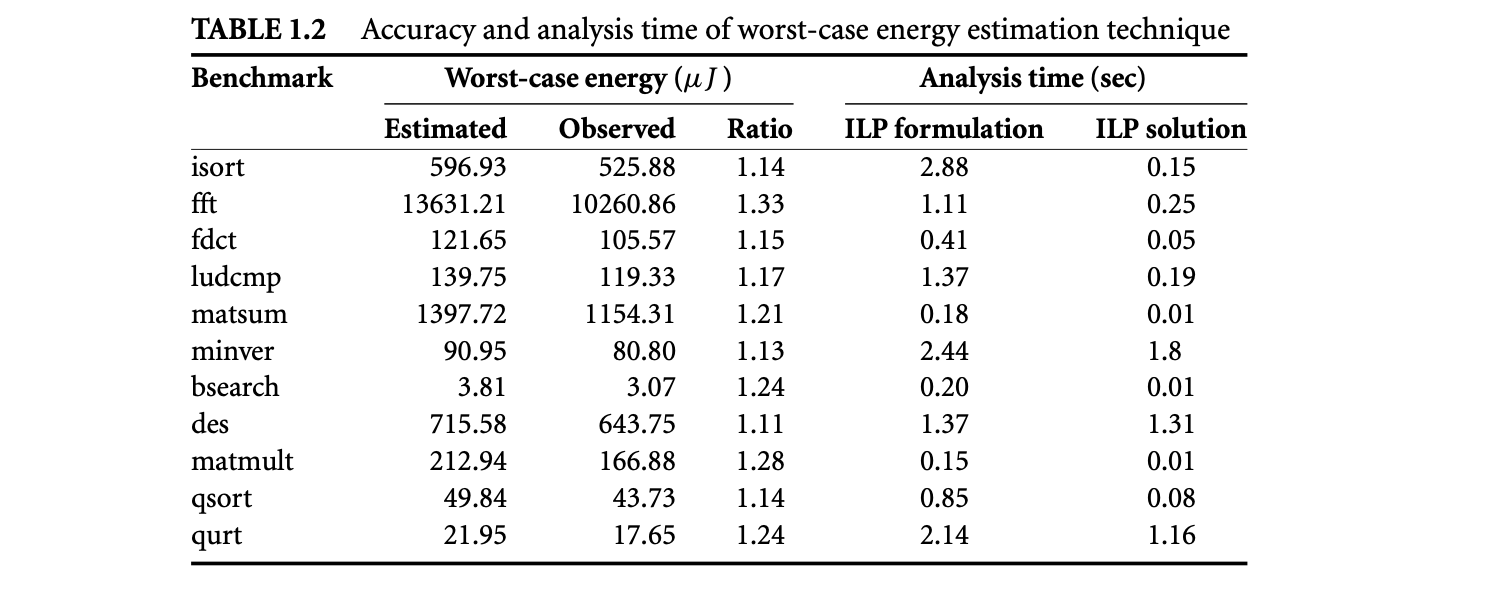
Table 1.2 presents the estimated worst-case energy obtained through static analysis and the observed worst-case energy obtained via simulation (Wattch simulator). The estimated values are quite close to the observed values. Moreover, the analysis is quite fast. It takes only seconds to formulate the ILP problems for the benchmark programs. The ILP solver (CPLEX) is even faster and completes in under 1.8 seconds for all the benchmarks. All the experiments have been performed on a Pentium IV 1.3 GHz PC with 1 GB of memory.
1.5 Existing WCET Analysis Tools
There are some commercial and research prototype tools for WCET analysis. We discuss them in this section. The most well known and extensively used commercial WCET analyzer is the aiT tool [1] from AbsInt Angewandte Informatik. aiT takes in a code snippet in executable form and computes its WCET. The analyzer uses a two-phased approach where micro-architectural modeling is performed first followed by path analysis. It employs abstract interpretation for cache/pipeline analysis and estimates an upper bound on the execution time of each basic block. These execution time bounds of basic blocks are then combined using ILP to estimate the WCET of the entire program. Versions of aiT are available for various platforms including Motorola PowerPC, Motorola ColdFire, ARM, and so on. The aiT tool is not open-source; so the user cannot change the analyzer code to model timing effects of new processor platforms. The main strength of the aiT tool is its detailed modeling of complex micro-architectures. It is probably the only WCET estimation tool to have a full modeling of the processor micro-architecture for a complex real-life processor like Motorola ColdFire [22] and Motorola PowerPC [32].
Another commercial WCET analyzer is the Bound-T tool [87], which also takes in binary executable programs. It concentrates mainly on program path analysis and does not model cache, complex pipeline, or branch prediction. In path analysis, an important focus of the tool is inferring loop bounds, for which it extensively uses the well-known Omega-calculator [66]. Bound-T has been targeted toward Intel 8051 series micro-controllers, Analog Devices ADSP-21020 DSP, and ATMEL ERC32 SPARC V7-based platforms. Like aiT, Bound-T is not open-source.
The Chronos WCET analyzer [44] incorporates timing models of different micro-architectural features present in modern processors. In particular, it models both in-order and out-of-order pipelines, instruction caches, dynamic branch prediction, and their interactions. The modeling of different architectural features is parameterizable. Chronos is a completely open-source distribution especially suited to the needs of the research community. This allows the researcher to modify and extend the tool for his or her individual needs. Current state-of-the-art WCET analyzers, such as aiT [1], are commercial tools that do not provide the source code. Unlike other WCET analyzers, Chronos is not targeted toward one or more commercial embedded processors. Instead, it is built on top of the freely available SimpleScalar simulator infrastructure. SimpleScalar is a widely popular cycle-accurate architectural simulator that allows the user
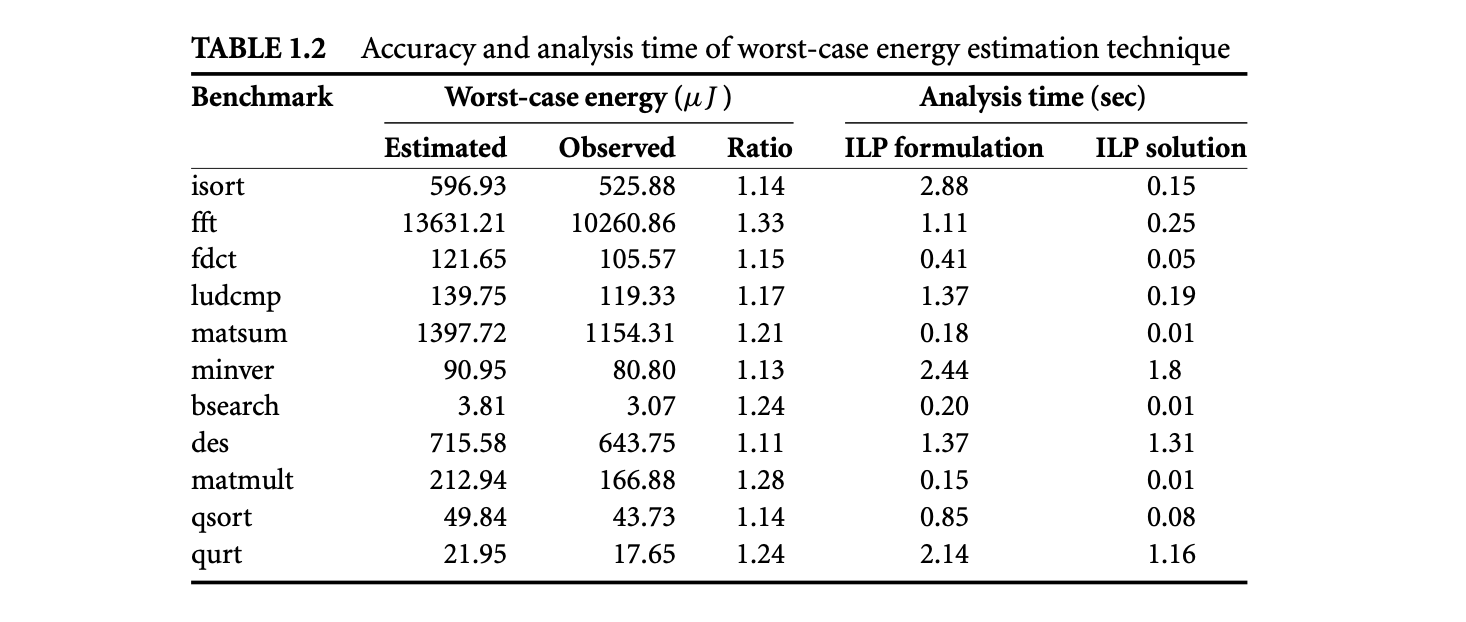
Table 1.2: Accuracy and analysis time of worst-case energy estimation technique to model a variety of processor platforms in software [10]. Chronos targets its analyzer to processor models supported by SimpleScalar. This choice of platform ensures that the user does not need to purchase a particular embedded platform and its associated compiler, debugger, and other tools (which are often fairly expensive) to conduct research in WCET analysis using Chronos. Also, the flexibility of SimpleScalar enables development and verification of modeling a variety of micro-architectural features for WCET analysis. Thus, Chronos provides a low-overhead, zero-cost, and flexible infrastructure for WCET research. However, it does not support as detailed micro-architectural modeling as is supported by the commercial aiT analyzer; in particular, certain processor features such as data cache are not modeled in Chronos.
Among the research prototypes, HEPTANE [64] is an open-source WCET analyzer. HEPTANE models in-order pipeline, instruction cache, and branch prediction, but it does not include any automated program flow analysis. Symta/P [77] is another research prototype that estimates WCET for C programs. It models caches and simple pipelines but does not support modeling of complex micro-architectural features such as out-of-order pipelines and branch prediction. Cinderella [48] is an ILP-based research prototype developed at Princeton University. The main distinguishing feature of this tool is that it performs both program path analysis and micro-architectural modeling by solving an ILP problem. However, this formulation makes the tool less scalable because the ILP solving time does not always scale up for complex micro-architectures. Also, Cinderella mostly concentrates on program path analysis and cache modeling; it does not analyze timing effects of complex pipelines and branch prediction. The SWET analyzer from Paderborn, Uppsala, and Malarden Universities focuses mostly on program flow analysis and does not model complex micro-architectures (such as out-of-order pipelines). The program flow analysis proceeds by abstract execution where variable values are abstracted to intervals. However, the abstraction in the flow analysis is limited to data values; the control flow is not abstracted. Consequently, abstract execution in the SWET tool [27] may resort to a complete unrolling of the program loops.
In addition to the above-mentioned tools, several other research groups have developed their own in-house timing analysis prototypes incorporating certain novel features. One notable effort is by the research group at Florida State University. Their work involves sophisticated flow analysis for inferring infeasible path patterns and loop bounds [31] -- features that are not commonly present in many WCET analyzers. However, the tool is currently not available for use or download; it is an in-house research effort.
1.6 Conclusions
In this chapter, we have primarily discussed software timing and energy analysis of an isolated task executing on a target processor without interruption. This is an important problem and forms the building blocks of more complicated performance analysis techniques. As we have seen, the main steps of software timing and energy analysis are (a) program path analysis and (b) micro-architectural modeling. We have also discussed a number of analysis methods that either perform an integrated analysis of the two steps or separate the two steps. It has been observed that integrated analysis methods are not scalable to large programs [94], and hence separated approaches for timing analysis may have a better chance of being integrated into compilers. Finally, we outline here some possible future research directions.
1.6.1 Integration with Schedulability Analysis
The timing and energy analysis methods discussed in this chapter assume uninterrupted execution of a program. In reality, a program (or "task," using the terminology of the real-time systems community) may get preempted because of interrupts. The major impact of task preemption is on the performance of the instruction and data caches. Let be a lower-priority task that gets preempted by a higher-priority task . When resumes execution, some of its cache blocks have been replaced by . Clearly, if the WCET analysis does not anticipate this preemption, the resulting timing guarantee will not be safe. Cache-related preemption delay[42, 58] analysis derives an upper bound on the number of additional cache misses per preemption. This information is integrated in the schedulability analysis [37] to derive the maximum number of possible preemptions and their effect on the worst-case cache performance.
1.6.2 System-Level Analysis
In a system-on-chip device consisting of multiple processing elements (typically on a bus), a system-wide performance analysis has to be built on top of task-level execution time analysis [70, 85]. Integrating the timing effects of shared bus and complex controllers in the WCET analysis is quite involved. In a recent work, Tanimoto et al. [80] model the shared bus on a system-on-chip device by defining bus scenario as representing a set of possible execution sequences of tasks and bus transfers. They use the definition of bus scenario to automatically derive the deadline and period for each task starting with high-level real-time requirements.
1.6.3 Retargetable WCET Analysis
Retargetability is one of the major issues that needs to be resolved for WCET analysis tools to gain wider acceptability in industry [12]. Developing a complex WCET analyzer for a new platform requires extensive manual effort. Unfortunately, the presence of a large number of platforms available for embedded software development implies that we cannot ignore this problem. The other related problem is the correctness of the abstract processor models used in static timing analysis. The manual abstraction process cannot guarantee the correctness of the models. These two problems can be solved if the static timing analyzer can be generated (semi-)automatically from a formal description of the processor.
One possibility in this direction is to start with the processor specification in some architecture description language (ADL). ADLs precisely describe the instruction-set architecture as well as the micro-architecture of a given processor platform. Certain architectural features are highly parameterizable and hence easy to retarget from a WCET analysis point of view, but other features such as out-of-order pipelines are not easily parameterizable. Li et al. [47] propose an approach to automatically generate static WCET analyzers starting from ADL descriptions for complex processor pipelines. On the other end of the spectrum, we can start with processor specification in hardware description languages (HDLs) such as Verilog or VHDL. The timing models have to be obtained from this HDL specification via simplification and abstraction. Thesing [84] takes this approach for timing models of a system controller. It remains to be seen whether this method scales to complex processor pipelines.
1.6.4 Time-Predictable System Design
The increasing complexity of systems and software leads to reduced timing predictability, which in turn creates serious difficulties for static analysis techniques [86]. An alternative is to design systems and software that are inherently more predictable in terms of timing without incurring significant performance loss. The Virtual Simple Architecture (VISA) approach [3] counters the timing anomaly problem in complex processor pipelines by augmenting the processor micro-architecture with a simpler pipeline. Proposals for predictable memory hierarchy include cache locking [89, 65], cache partitioning [95, 39], as well as replacing cache with scratchpad memory [90, 78] such that WCET analysis is simplified. At the software level, the work in [59, 28] discusses code transformations to reduce the number of program paths considered for WCET analysis. Moreover, Gustafsson et al. [28] also propose WCET-oriented programming to produce code with a very simple control structure that avoids input-data-dependent control flow decisions as far as possible.
1.6.5 WCET-Centric Compiler Optimizations
Traditional compiler optimization techniques guided by profile information focus on improving the average-case performance of a program. In contrast, the metric of importance to real-time systems is the worst-case execution time. Compiler techniques to reduce the WCET of a program have started to receive attention very recently. WCET-centric optimizations are more challenging, as the worst-case path changes as optimizations are applied.
Lee et al. [43] have developed a code generation method for dual-instruction-set ARM processors to simultaneously reduce the WCET and code size. They use a full ARM instruction set along the WCET path to achieve faster execution and at the same time we reduced Thumb instructions along the noncritical paths to reduce code size. Bodin and Puaut [8] designed a customized static branch prediction schemefor reducing a program's WCET. Zhao et al. [99] present a code positioning and transformation method to avoid the penalties associated with conditional and unconditional jumps by placing the basic blocks on WCET paths in contiguous positions whenever possible. Suhendra et al. [78] propose WCET-directed optimal and near-optimal variable allocation strategies to scratchpad memory. Finally, Yu and Mitra [97] exploit application-specific extensions to the base instruction set of a processor for reducing the WCET of real-time tasks. Clearly, there are many other contexts where WCET-guided compiler optimization can play a critical role.
Acknowledgments
Portions of this chapter were excerpted from R. Jayaseelan, T. Mitra, and X. Li, 2006, "Estimating the worst-case energy consumption of embedded software," in Proceedings of the 12th IEEE Real-Time and Embedded Technology and Applications Symposium (RTAS), pages 81-90, and adapted from X. Li, A. Roychoudhury, and T. Mitra, 2006, "Modeling out-of-order processors for WCET analysis," Real-Time Systems, 34(3): 195-227.
The authors would like to acknowledge Ramkumar Jayaseelan for preparing the figures in the introduction section.
References
[1] AbsInt Angewandte Informatik GmbH. aiT: Worst case execution time analyzer. http://www.absint.com/ait/.
[2] P. Altenbernd. 1996. On the false path problem in hard real-time programs. In Proceedings of the Eighth Euromicro Workshop on Real-Time Systems (ECRTS), 102-07.
[3] A. Anantaraman, K. Seth, K. Patil, E. Rotenberg, and F. Mueller. 2003. Virtual simple architecture (VISA): Exceeding the complexity limit in safe real-time systems. In Proceedings of the 30th IEEE/ACM International Symposium on Computer Architecture (ISCA), 350-61.
[4] R. Arnold, F. Mueller, D. B. Whalley, and M. G. Harmon. 1994. Bounding worst-case instruction cache performance. In Proceedings of the 15th IEEE Real-Time Systems Symposium (RTSS), 172-81.
[5] I. Bate and R. Reutemann. 2004. Worst-case execution time analysis for dynamic branch predictors. In Proceedings of the 16th Euromicro Conference on Real-Time Systems (ECRTS), 215-22.
[6] G. Bernat, A. Colin, and S. M. Petters. 2002. WCET analysis of probabilistic hard real-time systems. In Proceedings of the 23rd IEEE Real-Time Systems Symposium (RTSS), 279-88.
[7] R. Bodik, R. Gupta, and M. L. Soffa. 1997. Refining data flow information using infeasible paths. In Proceedings of the 6th European Software Engineering Conference held jointly with the 5th ACM SIGSOFT International Symposium on Foundations of Software Engineering ESEC/FSE, Vol. 1301 of Lecture Notes in Computer Science, 361-77. New York: Springer.
[8] F. Bodin and I. Pnuatt. 2005. A WCET-oriented static branch prediction scheme for real-time systems. In Proceedings of the 17th Euromicro Conference on Real-Time Systems, 33-40.
[9] D. Brooks, V. Tiwari, and M. Martonosi. 2000. Wattch: A framework for architectural-level power analysis and optimizations. In Proceedings of the 27th Annual ACM/IEEE International Symposium on Computer Architecture (ISCA), 83-94.
[10] D. Burger and T. Austin. 1997. The SimpleScalar tool set, version 2.0. Technical Report CS-TR-1997-1342, University of Wisconsin, Madison.
[11] C. Burguiere and C. Rochange. 2005. A contribution to branch prediction modeling in WCET analysis. In Proceedings of the IEEE Design, Automation and Test in Europe Conference and Exposition, Vol. 1, 612-17.
[12] K. Chen, S. Malik, and D. I. August. 2001. Retargetable static timing analysis for embedded software. In Proceedings of IEEE/ACM International Symposium on System Synthesis (ISSS).
[13] E. M. Clarke, E. A. Emerson, and A. P. Sistla. 1986. Automatic verification of finite-state concurrent systems using temporal logic specifications. ACM Transactions on Programming Languages and Systems 8(2):244-63.
[14] A. Colin and I. Pnuatt. 2000. Worst case execution time analysis for a processor with branch prediction. Real-Time Systems 18(2):249-74.
[15] P. Cousot and R. Cousot. 1977. Abstract interpretation: A unified lattice model for static analysis of programs by construction or approximation of fixpoints. In Proceedings of the Fourth Annual ACM Symposium on Principles of Programming Languages (POPL), 238-52.
[16] K. Dockser. 2001. "Honey, I shrunk the supercomputer!" -- The PowerPC 440 FPU brings supercomputing to IBM blue logic library. IBM MicroNews 7(4):27-29.
[17] S. Edgar and A. Burns. 2001. Statistical analysis of WCET for scheduling. In Proceedings of the 22nd IEEE Real-Time Systems Symposium (RTSS), 215-24.
[18] J. Eisinger, I. Polian, B. Becker, A. Metzner, S. Thesing, and R. Wilhelm. 2006. Automatic identification of timing anomalies for cycle-accurate worst-case execution time analysis. In Proceedings of the Ninth IEEE Workshop on Design and Diagnostics of Electronic Circuits and Systems (DDECS), 15-20.
[19] J. Engblom. 2003. Analysis of the execution time unpredictability caused by dynamic branch prediction. In Proceedings of the 9th IEEE Real-Time and Embedded Technology and Applications Symposium (RTAS), 152-59.
[20] J. Engblom and A. Ermedahl. 2000. Modeling complex flows for worst-case execution time analysis. In Proceedings of IEEE Real-Time Systems Symposium (RTSS).
[21] A. Ermedahl and J. Gustafsson. 1997. Deriving annotations for tight calculation of execution time. In Third International Euro-Par Conference on Parallel Processing (Euro-Par). Vol. 1300 of Lecture Notes in Computer Science, 1298-307. New York: Springer.
[22] C. Ferdinand, R. Heckmann, M. Langenbach, F. Martin, M. Schmidt, H. Theiling, S. Thesing, and R. Wilhelm. 2001. Reliable and precise WCET determination for a real-life processor. In Proceedings of International Workshop on Embedded Software (EMSOFT), 469-85.
[23] C. Ferdinand and R. Wilhelm. 1998. On predicting data cache behavior for real-time systems. In Proceedings of the ACM SIGPLAN Workshop on Languages, Compilers, and Tools for Embedded Systems (LCTES), 16-30.
[24] S. V. Gheorghita, T. Basten, and H. Corporaal. 2005. Intra-task scenario-aware voltage scheduling. In International Conference on Compiler, Architectures and Synthesis for Embedded Systems (CASES).
[25] S. V. Gheorghita, S. Stuijk, T. Basten, and H. Corporaal. 2005. Automatic scenario detection for improved WCET estimation. In ACM Design Automation Conference (DAC).
[26] S. Ghosh, M. Martonosi, and S. Malik. 1999. Cache miss equations: A compiler framework for analyzing and tuning memory behavior. ACM Transactions on Programming Languages and Systems, 21(4):707-46.
[27] J. Gustafsson. 2000. Eliminating annotations by automatic flow analysis of real-time programs. In Proceedings of the Seventh International Conference on Real-Time Computing Systems and Applications (RTCSA), 511-16.
[28] J. Gustafsson, B. Lisper, R. Kirner, and P. Puschner. 2006. Code analysis for temporal predictability. Real-Time Systems 32:253-77.
[29] C. Healy, R. Arnold, F. Mueller, D. Whalley, and M. Harmon. 1999. Bounding pipeline and instruction cache performance. IEEE Transactions on Computers 48(1):53-70.
[30] C. Healy, M. Sjodin, V. Rustagi, D. Whalley, and R. van Englen. 2000. Supporting timing analysis by automatic bounding of loop iterations. Real-Time Systems 18:129-56.
[31] C. A. Healy and D. B. Whalley. 2002. Automatic detection and exploitation of branch constraints for timing analysis. IEEE Transactions on Software Engineering 28(8):763-81.
[32] R. Heckmann, M. Langenbach, S. Thesing, and R. Wilhelm. 2003. The influence of processor architecture on the design and the results of WCET tools. Proceedings of the IEEE, 91(7):1038-054.
[33] J. L. Hennessy and D. A. Patterson. 2003. Computer architecture -- a quantitative approach. 3rd ed. San Francisco: Morgan Kaufmann.
[34] IBM Microelectronics Division. 1999. The PowerPC 440 core.
[35] Institute of Electrical and Electronics Engineers. 1985. IEEE 754: Standard for binary floating-point arithmetic.
[36] R. Jayaseelan, T. Mitra, and X. Li. 2006. Estimating the worst-case energy consumption of embedded software. In Proceedings of the 12th IEEE Real-Time and Embedded Technology and Applications Symposium (RTAS), 81-90.
[37] L. Ju, S. Chakraborty, and A. Roychoudhury. 2007. Accounting for cache-related preemption delay in dynamic priority schedulability analysis. In Proceedings of Design Automation and Test in Europe (DATE).
[38] S.-K. Kim, S. L. Min, and R. Ha. 1996. Efficient worst case timing analysis of data caching. In Proceedings of the Second IEEE Real-Time Technology and Applications Symposium (RTAS), 230-40.
[39] D. B. Kirk. 1989. SMART (strategic memory allocation for real-time) cache design. In Proceedings of the Real-Time Systems Symposium (RTSS), 229-39.
[40] R. Kirner. 2003. Extending optimizing compilation to support worst-case execution time analysis. PhD thesis, T. U. Vienna.
[41] M. Langenbach, S. Thesing, and R. Heckmann. Pipeline modeling for timing analysis. In Proceedings of the 9th International Symposium on Static Analysis (SAS). Vol. 2477 of Lecture Notes in Computer Science, 294-309. New York: Springer.
[42] C.-G. Lee, H. Hahn, Y.-M. Seo, S. L. Min, R. Ha, S. Hong, C. Y. Park, M. Lee, and C. S. Kim. 1998. Analysis of cache-related preemption delay in fixed-priority preemptive scheduling. IEEE Transactions on Computers 47(6):700-13.
[43] S. Lee et al. 2004. A flexible tradeoff between code size and WCET using a dual instruction set processor. In Proceedings of the 8th International Workshop on Software and Compilers for Embedded Systems (SCOPES). Vol. 3199 of Lecture Notes in Computer Science, 244-58. New York: Springer.
[44] X. Li, Y. Liang, T. Mitra, and A. Roychoudhury. Chronos: A timing analyzer for embedded software. Science of Computer Programming, special issue on Experiment Software and Toolkit 2007 (to appear), http://www.comp.nus.edu.sg/rpembed/chronos/.
[45] X. Li, T. Mitra, and A. Roychoudhury. 2005. Modeling control speculation for timing analysis. Real-Time Systems 29(1):27-58.
[46] X. Li, A. Roychoudhury, and T. Mitra. 2006. Modeling out-of-order processors for WCET analysis. Real-Time Systems 34(3):195-227.
[47] X. Li, A. Roychoudhury, T. Mitra, P. Mishra, and X. Cheng. 2007. A retargetable software timing analyzer using architecture description language. In Proceedings of the 12th Asia and South Pacific Design Automation Conference (ASP-DAC), 396-401.
[48] Y.-T. S. Li. Cinderella 3.0 WCET analyzer. http://www.princeton.edu/yaudil/cinderella-3.0/.
[49] Y.-T. S. Li and S. Malik. 1997. Performance analysis of embedded software using implicit path enumeration. IEEE Transactions on Computer-Aided Design of Integrated Circuits and Systems (TCAD) 16(12):1477-87.
[50] Y.-T. S. Li and S. Malik. 1998. Performance analysis of real-time embedded software. New York: Springer.
[51] S.-S. Lim, Y. H. Bae, G. T. Jang, B-D. Rhee, S. L. Min, C. Y. Park, H. Shin, K. Park, S.-M. Moon, and C. S. Kim. 1995. An accurate worst case timing analysis for RISC processors. IEEE Transactions on Software Engineering 21(7):593-604.
[52] Y. A. Liu and G. Gomez. 2001. Automatic accurate cost-bound analysis for high-level languages. IEEE Transactions on Computers 50(12):1295-309.
[53] T. Lundqvist and P. Stenstrom. 1999. An integrated path and timing analysis method based on cycle-level symbolic execution. Real-Time Systems 17(2/3):183-207.
[54] T. Lundqvist and P. Stenstrom. 1999. Timing anomalies in dynamically scheduled microprocessors. In Proceedings of the 20th IEEE Real-Time Systems Symposium (RTSS), 12-21.
[55] F. Martin, M. Alt, R. Wilhelm, and C. Ferdinand. 1998. Analysis of loops. In Compiler Construction (CC). New York: Springer.
[56] A. Metzner. 2004. Why model checking can improve WCET analysis. In Proceedings of the 16th International Conference on Computer Aided Verification (CAV). Vol. 3114 of Lecture Notes in Computer Science, 361-71. New York: Springer.
[57] F. Mueller. 2000. Timing analysis for instruction caches. Real-Time Systems 18:217-47.
[58] H. S. Negi, T. Mitra, and A. Roychoudhury. 2003. Accurate estimation of cache-related preemption delay. In Proceedings of the 1st IEEE/ACM/IFIP International Conference on Hardware/Software Codesign and System Synthesis (CODES+ISSS), 201-06.
[59] H. S. Negi, A. Roychoudhury, and T. Mitra. 2004. Simplifying WCET analysis by code transformations. In Proceedings of the 4th International Workshop on Worst-Case Execution Time Analysis (WCET).
[60] G. Ottosson and M. Sjodin. 1997. Worst-case execution time analysis for modern hardware architectures. In Proceedings of the ACM SIGPLAN Workshop on Languages, Compilers, and Tools for Real-Time Systems (LCT-RTS).
[61] C. Y. Park. 1993. Predicting program execution times by analyzing static and dynamic program paths. Real-time Systems 5(1):31-62.
[62] C. Y. Park. 1992. Predicting deterministic execution times of real-time programs. PhD thesis, University of Washington, Seattle.
[63] J. Pierce and T. Mudge. 1996. Wrong-path instruction prefetching. In Proceedings of the 29th Annual IEEE/ACM International Symposium on Microarchitectures (MICRO), 165-75.
[64] I. Pnuaut. HEPTANE static WCET analyzer. http://www.irisa.fr/aces/work/heptane-demo/heptane.html.
[65] I. Pnuaut and D. Decotigny. 2002. Low-complexity algorithms for static cache locking in multi-tasking hard real-time systems. In Proceedings of the 23rd IEEE Real-Time Systems Symposium (RTSS), 114-23.
[66] W. Pugh. 1991. The omega test: A fast and practical integer programming algorithm for dependence analysis. In ACM/IEEE Conference on Supercomputing.
[67] P. Puschner and C. Koza. 1989. Calculating the maximum execution time of real-time programs. Real-Time Systems 1(2):159-76.
[68] P. Puschner and A. Schedl. 1997. Computing maximum task execution times: A graph based approach. Real-Time Systems 13(1):67-91.
[69] H. Ramaprasad and F. Mueller. Bounding worst-case data cache behavior by analytically deriving cache reference patterns. In IEEE Real-Time Technology and Applications Symposium (RTAS), 148-57.
[70] K. Richter, D. Ziegenbein, M. Jersak, and R. Ernst. 2002. Model composition for scheduling analysis in platform design. In Proceedings of the 39th Annual ACM/IEEE Design Automation Conference (DAC), 287-92.
[71] A. Roychoudhury, T. Mitra, and H. S. Negi. 2005. Analyzing loop paths for execution time estimation. In Lecture Notes in Computer Science. Vol. 3816, 458-69. New York: Springer.
[72] T. Schuele and K. Schneider. 2004. Abstraction of assembler programs for symbolic worst case execution time analysis. In Proceedings of the 41st ACM/IEEE Design Automation Conference (DAC), 107-12.
[73] A. C. Shaw. 1989. Reasoning about time in higher-level language software. IEEE Transactions on Software Engineering 1(2):875-89.
[74] Simplify. Simplify theorem prover. http://www.research.compaq.com/SRC/esc/Simplify.html.
[75] A. Sinha and A. P. Chandrakasan. 2001. Jouletrack: A web based tool for software energy profiling. In Proceedings of the Design Automation Conference (DAC).
[76] F. Stappert, A. Ermedahl, and J. Engblom. 2001. Efficient longest executable path search for programs with complex flows and pipeline effects. In Proceedings of the First International Conference on Compilers, Architecture, and Synthesis for Embedded Systems (CASES), 132-40.
[77] J. Staschulat. Symta/P: Symbolic timing analysis for processes. http://www.ida.ing.tu-bs.de/research/projects/symta/home.e.shtml.
[78] V. Suhendra, T. Mitra, A. Roychoudhury, and T. Chen. 2005. WCET centric data allocation to scratchpad memory. In Proceedings of the 26th IEEE Real-Time Systems Symposium (RTSS), 223-32.
[79] V. Suhendra, T. Mitra, A. Roychoudhury, and T. Chen. 2006. Efficient detection and exploitation of infeasible paths for software timing analysis. In Proceedings of the 43rd ACM/IEEE Design Automation Conference (DAC), 358-63.
[80] T. Tanimoto, S. Yamaguchi, A. Nakata, and T. Higashino. 2006. A real time budgeting method for module-level-pipelined bus based system using bus scenarios. In Proceedings of the 43rd ACM/IEEE Design Automation Conference (DAC), 37-42.
[81] H. Theiling and C. Ferdinand. 1998. Combining abstract interpretation and ILP for microarchitecture modelling and program path analysis. In Proceedings of the 19th IEEE Real-Time Systems Symposium (RTSS), 144-53.
[82] H. Theiling, C. Ferdinand, and R. Wilhelm. 2000. Fast and precise WCET prediction by separated cache and path analyses. Real-Time Systems 18(2/3):157-79.
[83] S. Thesing. Safe and precise worst-case execution time prediction by abstract interpretation of pipeline models. PhD thesis, University of Saarland, Germany.
[84] S. Thesing. 2006. Modeling a system controller for timing analysis. In Proceedings of the 6th ACM/IEEE International Conference on Embedded Software (EMSOFT), 292-300.
[85] L. Thiele, S. Chakraborty, M. Gries, A. Maxiaguine, and J. Greuert. 2001. Embedded software in network processors -- models and algorithms. In Proceedings of the First International Workshop on Embedded Software (EMSOFT). Vol. 2211 of Lecture Notes in Computer Science, 416-34. New York: Springer.
[86] L. Thiele and R. Wilhelm. 2004. Design for timing predictability. Real-Time Systems, 28(2/3):157-77.
[87] Tidorum Ltd. Bound-T execution time analyzer. http://www.bound-t.com.
[88] V. Tiwari, S. Malik, and A. Wolfe. 1994. Power analysis of embedded software: A first step towards software power minimization. IEEE Transactions of VLSI Systems 2(4):437-45.
[89] X. Vera, B. Lisper, and J. Xue. 2003. Data cache locking for higher program predictability. In Proceedings of the International Conference on Measurements and Modeling of Computer Systems (SIGMETRICS), 272-82.
[90] L. Wehmeyer and P. Marwedel. 2005. Influence of memory hierarchies on predictability for time constrained embedded software. In Proceedings of the Conference on Design, Automation and Test in Europe (DATE), 600-605.
[91] I. Wenzel, R. Kirner, P. Puschner, and B. Rieder. 2005. Principles of timing anomalies in superscalar processors. In Proceedings of the Fifth International Conference on Quality Software (QSIC), 295-303.
[92] I. Wenzel, R. Kirner, B. Rieder, and P. Puschner. Measurement-based worst-case execution time analysis. In Proceedings of the Third IEEE Workshop on Software Technologies for Future Embedded and Ubiquitous Systems (SEUS), 7-10.
[93] R. White, F. Mueller, C. Healy, D. Whalley, and M. Harmon. 1997. Timing analysis for data caches and set-associative caches. In Proceedings of the Third IEEE Real-Time Technology and Applications Symposium (RTAS), 192-202.
[94] R. Wilhelm. 2004. Why AI + ILP is good for WCET, but MC is not, nor ILP alone. In Proceedings of the 5th International Conference on Verification, Model Checking, and Abstract Interpretation (VMCAI). Vol. 2937 of Lecture Notes in Computer Science, 309-22. New York: Springer.
[95] A. Wolfe. 1994. Software-based cache partitioning for real-time applications. Journal of Computer and Software Engineering, Special Issue on Hardware-Software Codesign, 2(3):315-27.
[96] W. Ye et al. 2000. The design and use of simplepower: A cycle-accurate energy estimation tool. In Proceedings of the ACM/IEEE Design Automation Conference (DAC).
[97] P. Yu and T. Mitra. 2005. Satisfying real-time constraints with custom instructions. In Proceedings of the ACM International Conference on Hardware/Software Codesign and System Synthesis (CODES+ISSS), 166-71.
[98] Y. Zhang et al. 2003. Hotleakage: A temperature-aware model of subthreshold and gate leakage for architects. Technical Report CS-2003-05, University of Virginia.
[99] W. Zhao, D. Whalley, C. Healy, and F. Mueller. 2004. WCET code positioning. In Proceedings of the 25th IEEE Real-Time Systems Symposium (RTSS), 81-91.
2. Static Program Analysis for Security
Abstract
In this chapter, we discuss static analysis of the security of a system. First, we give a brief background on what types of static analysis are feasible in principle and then move on to what is practical. We next discuss static analysis of buffer overflow and mobile code, followed by access control. Finally, we discuss static analysis of information flow expressed in a language that has been annotated with flow policies.
2.1 Introduction
Analyzing a program for security holes is an important part of the current computing landscape, as security has not been an essential ingredient in a program's design for quite some time. With the critical importance of a secure program becoming clearer in the recent past, designs based on explicit security policies are likely to gain prominence.
Static analysis of a program is one technique to detect security holes. Compared to monitoring an execution at runtime (which may not have the required coverage), a static analysis -- even if incomplete because of loss of precision -- potentially gives an analysis on all runs possible instead of just the ones seen so far.
However, security analysis of an arbitrary program is extremely hard. First, what security means is often unspecified or underspecified. The definition is either too strict and cannot cope with the "commonsense" requirement or too broad and not useful. For example, one definition of security involves the notion of "noninterference" [24]. If it is very strict, even cryptoanalytically strong encryption and decryption does not qualify as secure, as there is information flow from encrypted text to plain text [59]. If it is not very strict, by definition, some flows are not captured that are important in some context for achieving security and hence, again, not secure. For example, if electromagnetic emissions are not taken into account, the key may be easily compromised [50]. A model of what security means is needed, and this is by no means an easy task [8]. Schneider [28] has a very general definition: a security policy defines a binary partition of all (computable) sets of executions -- those that satisfy and those that do not. This is general enough to cover access control policies (a program's behavior on an arbitrary individual execution for an arbitrary finite period), availability policies (behavior on an arbitrary individual execution over an infinite period), and information flow (behavior in terms of the set of all executions).
Second, the diagonalization trick is possible, and many analyses are undecidable. For example, there are undecidable results with respect to viruses and malicious logic [16]: it is undecidable whether an arbitrary program contains a computer virus. Similarly, viruses exist for which no error-free detection algorithm exists.
Recently, there have been some interesting results on computability classes for enforcement mechanisms [28] with respect to execution monitors, program rewriting, and static analysis. Execution monitors intervene whenever execution of an untrusted program is about to violate the security policy being enforced. They are typically used in operating systems using structures such as access control lists or used when executing interpreted languages by runtime type checking. It is possible to rewrite a binary so that every access to memory goes through a monitor. While this can introduce overhead, optimization techniques can be used to reduce the overhead. In many cases, the test can be determined to be not necessary and removed by static analysis. For example, if a reference to a memory address has already been checked, it may not be necessary for a later occurrence.
Program rewriting modifies the untrusted program before execution to make it incapable of violating the security policy. An execution monitor can be viewed as a special case of program rewriting, but Hamlen et al. [28] point out certain subtle cases. Consider a security policy that makes halting a program illegal; an execution monitor cannot enforce this policy by halting, as this would be illegal! There are also classes of policies in certain models of execution monitors that cannot be enforced by any program rewriter.
As is to be expected, the class of statically enforceable policies is the class of recursively decidable properties of programs (class of the arithmetic hierarchy): a static analysis has to be necessarily total (i.e., terminate) and return safe or unsafe. If precise analysis is not possible, we can relax the requirement by being conservative in what it returns (i.e., tolerate false positives). Execution monitors are the class of co-recursively enumerable languages (class of the arithmetic hierarchy).1
A security policy is co-recursively enumerable if there exists a Turing machine that takes an arbitrary execution monitor as an input and rejects it in finite time if ; otherwise loops forever.
A system's security is specified by its security policy (such as access control or information flow model) and implemented by mechanisms such as physical separation or cryptography.2 Consider access control. An access control system guards access to resources, whereas an information flow model classifies information to prevent disclosure. Access control is a component of security policy, while cryptography is one technical mechanism to effect the security policy. Systems have employed basic access control since timesharing systems began (1960) (e.g., Multics, Unix). Simple access control models for such "stand-alone" machines assumed the universe of users known, resulting in the scale of the model being "small." A set of access control moves can unintentionally leak a right (i.e., give access when it should not). If it is possible to analyze the system and ensure that such a result is not possible, the system can be said to be secure, but theoretical models inspired by these systems (the most well known being the Harrison, Ruzzo, Ullman [HRU] model) showed "surprising" undecidability results [29], chiefly resulting from the unlimited number of subjects and objects possible. Technically, in this model, it is undecidable whether a given state of a given protection system is safe for a given generic right. However, the need for automated analysis of policies was small in the past, as the scale of the systems was small.
While cryptography has rightfully been a significant component in the design of large-scale systems, its relation to security policy, especially its complementarity, has not often been brought out in full. “If you think cryptography is the solution to your problem, you don’t know what your problem is” (Roger Needham).
Information flow analysis, in contrast to access control, concerns itself with the downstream use of information once obtained after proper access control. Carelessness in not ensuring proper flow models has resulted recently in the encryption system in HD-DVD and BluRay disks to be compromised (the key protecting movie content is available in memory).3
The compromise of the security system DeCSS in DVDs was due to cryptanalysis, but in the case of HD-DVD it was simply improper information flow.
Overt models of information flow specify the policy concerning how data should be used explicitly, whereas covert models use "signalling" of information through "covert" channels such as timing, electromagnetic emissions, and so on. Note that the security weakness in the recent HD-DVD case is due to improper overt information flow. Research on some overt models of information flow such as Bell and LaPadula's [6] was initiated in the 1960s, inspired by the classification of secrets in the military. Since operating systems are the inspiration for work in this area, models of secure operating systems were developed such as C2 and B2 [57]. Work on covert information flow progressed in the 1970s. However, the work on covert models of information flow in proprietary operating systems (e.g., DG-UNIX) was expensive and too late, so late that it could not be used on the by then obsolescent hardware. Showing that Trojan horses did not use covert channels to compromise information was found to be "ultimately unachievable" [27].
Currently, there is a considerable interest in studying overt models of information flow, as the extensive use of distributed systems and recent work with widely available operating systems such as SELinux and OpenSolaris have expanded the scope of research. The scale of the model has become "large," with the need for automated analysis of policies being high.
Access control and information flow policies can both be statically analyzed, with varying effectiveness depending on the problem. Abstract interpretation, slicing, and many other compiler techniques can also be used in conjunction. Most of the static analyses induce a constraint system that needs to be solved to see if security is violated. For example, in one buffer overflow analysis [23], if there is a solution to a constraint system, then there is an attack. In another analysis in language-based security, nonexistence of a solution to the constraints is an indication of a possible leak of information.
However, static analysis is not possible in many cases [43] and has not yet been used on large pieces of software. Hence, exhaustive checking using model checking [14] is increasingly being used when one wants to gain confidence about a piece of code. In this chapter, we consider model checking as a form of static analysis. We will discuss access control on the Internet that uses model checking (Section 2.4.4). We will also discuss this approach in the context of Security-Enhanced Linux (SELinux) where we check if a large application has been given only sufficient rights to get its job done [31].
In spite of the many difficulties in analyzing the security of a system, policy frameworks such as access control and information flow analysis and mechanisms such as cryptography have been used to make systems "secure." However, for any such composite solution, we need to trust certain entities in the system such as the compiler, the BIOS, the (Java) runtime system, the hardware, digital certificates, and so on -- essentially the "chain of trust" problem. That this is a tricky problem has been shown in an interesting way by Ken Thompson [53]; we will discuss it below. Hence, we need a "small" trusted computing base (TCB): all protection mechanisms within a system (hardware, software, firmware) for enforcing security policies.
In the past (early 1960s), operating systems were small and compilers larger in comparison. The TCB could justifably be the operating system, even if uncomfortably larger than one wished. In today's context, the compilers need not be as large as current operating systems (for example, Linux kernel or Windows is many millions of lines of code), and a TCB could profitably be the compiler. Hence, a compiler analysis of security is meaningful nowadays and likely to be the only way large systems (often a distributed system) can be crafted in the future. Using a top-level security policy, it may be possible to automatically partition the program so that the resulting distributed system is secure by design [60].
To illustrate the effectiveness of static security analysis, we first discuss a case where static analysis fails completely (Ken Thomson's Trojan horse). We then outline some results on the problem of detecting viruses and then discuss a case study in which static analysis can in principle be very hard (equivalent to cryptanalysis in general) but is actually much simpler because of a critical implementation error. We will also briefly touch upon obfuscation that exploits difficulty of analysis.
We then discuss static analysis of buffer overflows, loading of mobile code, and access control and information flow, illustrating the latter using Jif [35] language on a realistic problem. We conclude with likely future directions in this area of research.
2.1.1 A Dramatic Failure of Static Analysis: Ken Thompson's Trojan Horse
Some techniques to defeat static analysis can be deeply effective; we summarize Ken Thompson's ingenious Trojan horse trick [53] in a compiler that uses self-reproduction, self-learning, and self-application. We follow his exposition closely.
First, self-reproduction is possible; for example, one can construct a self-reproducing program such as ((lambda x. (list x x)) (lambda x. (list x x))). Second, it is possible to teach a compiler (written in its own language) to compile new features (the art of bootstrapping a compiler): this makes self-learning possible. We again give Ken Thompson's example to illustrate this. Let us say that a lexer knows about '\n' (newline) but not '\v' (vertical tab). How does one teach it to compile '\v' also? Let the initial source be:
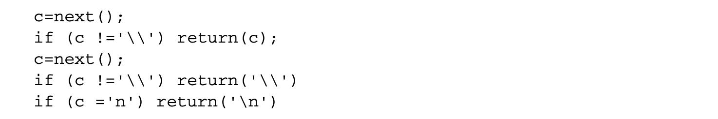
Adding to the compiler source

and using previous compiler binary does not work, as that binary does not know about '\v'. However, the following works:

Now a new binary (from the new source using the old compiler binary) knows about '\v' in a portable way. Now we can use it to compile the previously uncompilable statement:

The compiler has "learned." Now, we can introduce a Trojan horse into the login program that has a backdoor to allow a special access to log in as any user:
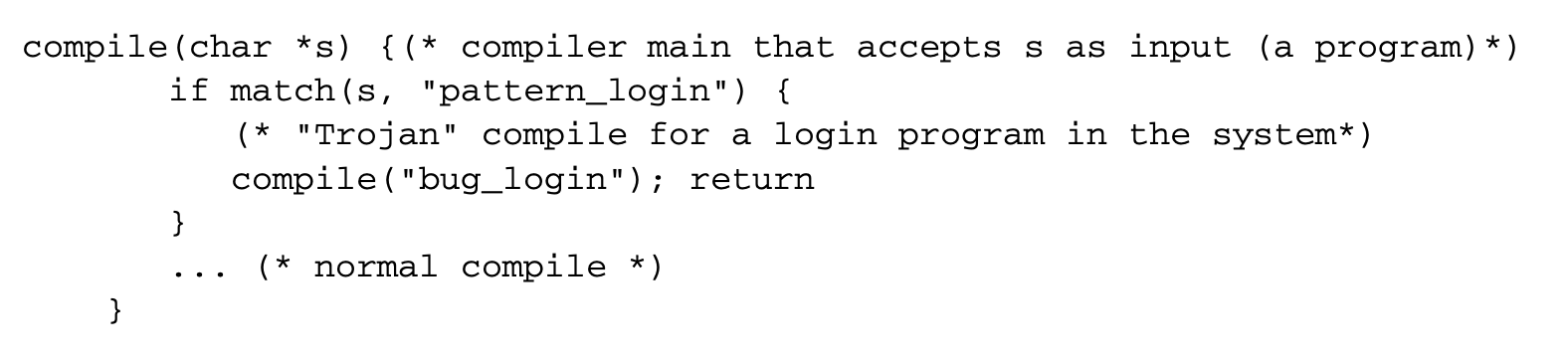
However, this is easily detectable (by examining the source). To make this not possible, we can add a second Trojan horse aimed at the compiler:
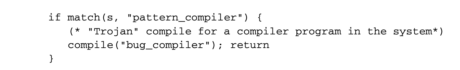
Now we can code a self-reproducing program that reintroduces both Trojan horses into the compiler with a learning phase where the buggy compiler binary with two Trojan horses now reinserts it into any new compiler binary compiled from a clean source! The detailed scheme is as follows: first a clean compiler binary (A) is built from a clean compiler source (S). Next, as part of the learning phase, a modified compiler source () can be built that incorporates the bugs. The logic in S' looks at the source code of any program submitted for compilation and, say by pattern matching, decides whether a program submitted is a login or a compiler program. If it decides that it is one of these special programs, it reproduces4 one or more Trojan horses (as necessary) when presented with a clean source. Let the program be compiled with A. We have a new binary A' that reinserts the two Trojans on any clean source!
It is easiest to do so in the binary being produced as the compiled output.
The virus exists in the binary but not in the source. This is not possible to discern unless the history of the system (the sequence of compilations and alterations) is kept in mind. Static analysis fails spectacularly!
2.1.2 Detecting Viruses
As discussed earlier, the virus detection problem is undecidable. A successful virus encapsulates itself so that it cannot be detected -- the opposite of "self-identifying data." For example, a very clever virus would put logic in I/O routines so that any read of suspected portions of a disk returns the original "correct" information! A polymorphic virus inserts "random" data to vary the signature. More effectively, it can create a random encryption key to encrypt the rest of the virus and store the key with the virus.
Cohen's ResultsCohen's impossibility result states that it is impossible for a program to perfectly demarcate a line, enclosing all and only those programs that are infected with some virus: no algorithm can properly detect all possible viruses [16]: does not detect Virus. For any candidate computer virus detection algorithm , there is a program p(pgm): if A(pgm) then exit; else spread. Here, spread means behave like a virus. We can diagonalize this by setting pgm=p and a contradiction follows immediately as p spreads iff not A(p).
Similarly, Chess and White [11] show there exists a virus that no algorithm perfectly detects, i.e., one with no false positives: . does not detect Virus. Also, there exists a virus that no algorithm loosely detects, i.e., claims to find the virus but is infected with some other virus: . does not loosely-detect Virus. In other words, there exist viruses for which, even with the virus analyzed completely, no program detects only that virus with no false positives. Further, another Chess and White's impossibility result states that there is no program to classify programs (only those) with a virus V and not include any program without any virus.
Furthermore, there are interesting results concerning polymorphic viruses: these viruses generate a set of other viruses that are not identical to themselves but are related in some way (for example, are able to reproduce the next one in sequence). If the size of this set is greater than 1, call the set of viruses generated the viral set S.
An algorithm detects a set of viruses iff for every program , terminates and returns TRUE iff is infected with some virus in . If is a polyvirus, for any candidate -detection algorithm , there is a program that is an instance of :
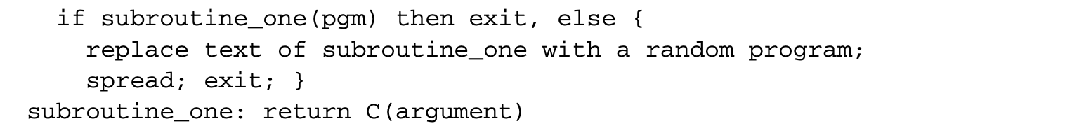
This can be diagonalized by , resulting in a contradiction: if C(s) true exit; other-wise polyvirus.
Hence, it is clear that static analysis has serious limits.
2.1.3 A Case Study for Static Analysis: GSM Security Hole
We will now attempt to situate static analysis with other analyses, using the partitioning attack [50] on GSM hashing on a particular implementation as an example. GSM uses the COMP128 algorithm for encryption. A 16B (128b) key of subscriber (available with the base station along with a 16B challenge from the base station is used to construct a 12B (96b) hash. The first 32b is sent as a response to the challenge, and the remaining 64b is used as the session key. The critical issue is that there should be no leakage of the key in any of the outputs this includes any electromagnetic (EM) leakages during the computation of the hash. The formula for computation of the hash it has a butterfly structure) is as follows:
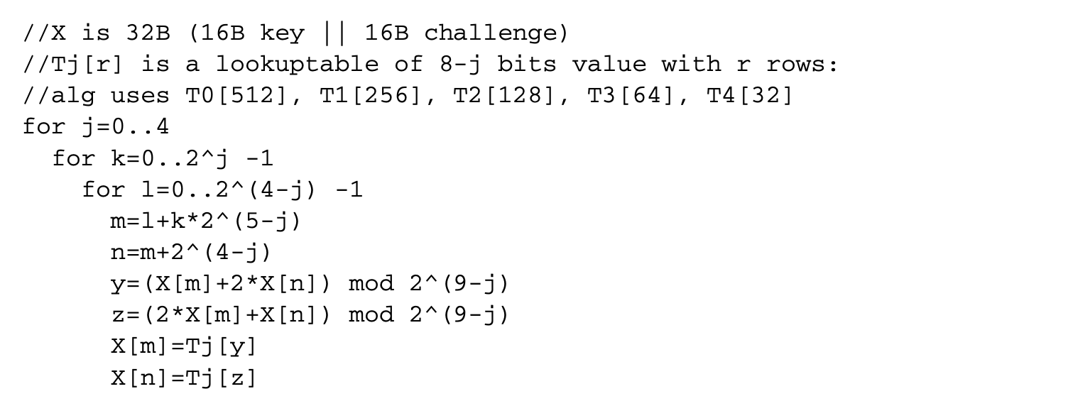
If we expand y in the expression for X[m], we have

A simple-minded flow analysis will show that there is direct dependence of the EM leakage on the key; hence, this is not information flow secure. However, cryptographers, using the right "confusion" and "diffusion" operators such as the above code, have shown that the inverse can be very difficult to compute. Hence, even if very simple static analysis clearly points out the flow dependence of the EM leakage on the key, it is not good enough to crack the key. However, even if the mapping is cryptanalytically strong, "implementation" bugs can often give away the key. An attack is possible if one does not adhere to the following principle [50] of statistical independence (or more accurately noninterference, which will be discussed later): relevant bits of all intermediate cycles and their values should be statistically independent of the inputs, outputs, and sensitive information.
Normally, those bits that emit high EM are good candidates for analysis. One set of candidates are the array and index values, as they need to be amplified electrically for addressing memory. They are therefore EM sensitive, whereas other internal values may not be so.
Because of the violation of this principle, a cryptographically strong algorithm may have an implementation that leaks secrets. For example, many implementations use 8b microprocessors, as COMP128 is optimized for them, so the actual implementation for T0 is two tables, T00 and T01 (each 256 entries):
If the number of intermediate lookups from tables T00 or T01 have statistical significance, then because of the linearity of the index y with respect to R for the first round, some information can be gleaned about the key. The technique of differential cryptanalysis is based on such observations. In addition, if it is possible to know when access changes from one table (say, T00) to another (T01) by changing R, then the R value where it changes is given by K + 2*R=256, from which X, the first byte of the GSM key, can be determined.
In general, we basically have a set of constraints, such as

where and are two close values that map the index into different arrays (T0 or T1).5
In general, , with being an affine function for tractability.
If there is a solution to these Diophantine equations, then we have an attack. Otherwise, no. Since the cryptographic confusion and diffusion operations determine the difficulty (especially with devices such as S-boxes in DES), in general the problem is equivalent to the cryptanalysis problem. However, if we assume that the confusion and diffusion operations are linear in subkey and other parameters (as in COMP128), we just need to solve a set of linear Diophantine equations [39].
What we can learn from the above is the following: we need to identify EM-sensitive variables. Other values can be "dclassified"; even if we do not take any precautions, we can assume they cannot be observed from an EM perspective. We need to check the flow dependence of the EM-sensitive variables (i.e., externally visible) on secrets that need to be safeguarded.
Recently, work has been done that implies that success or failure of branch prediction presents observable events that can be used to crack encryption keys.
The above suggests the following problems for study:
- Automatic downgrading of "insensitive" variables
- Determination of the minimal declassification to achieve desired flow properties
2.1.4 Obfuscation
Given that static analyses are often hard, some applications use them to good effect. An example is the new area of "obfuscation" of code so that it cannot be reverse-engineered easily. Obfuscation is the attempt to make code "unreadable" or "unintelligible" in the hope that it cannot be used by competitors. This is effected by performing semantic-preserving transformations so that automatic static analysis can reveal nothing useful. In one instance, control flow is intentionally altered so that it is difficult to understand or use it by making sure that any analysis that can help in unravelling code is computationally intractable (for example, PSPACE-hard or NP-hard). Another example is intentionally introducing aliases, as certain alias analysis problems are known to be hard (if not undecidable), especially in the interprocedural context. Since it has been shown that obfuscation is, in general, impossible [4], static analysis in principle could be adopted to undo obfuscation unless it is computationally hard.
2.2 Static Analysis of Buffer Overflows
Since the advent of the Morris worm in 1988, buffer overflow techniques to compromise systems have been widely used. Most recently, the SQL slammer worm in 2003, using a small UDP packet (376B), compromised 90% of all target machines worldwide in less than 10 minutes.
Since buffer overflow on a stack can be avoided, for example, by preventing the return address from being overwritten by the "malicious" input string, array bounds checking the input parameters by the callee is one technique. Because of the cost of this check, it is useful to explore compile time approaches that eliminate the check through program analysis. Wagner et al. [56] use static analysis (integer range analysis), but it has false positives due to imprecision in pointer analysis, interprocedural analysis, and so on and a lack of information on dynamically allocated sizes.
CCured [46] uses static analysis to insert runtime checks to create a type-safe version of C program. CCured classifies C pointers into SAFE, SEQ, or WILD pointers. SAFE pointers require only a null check. SEQ pointers require a bounds check, as these are involved in pointer arithmetic, but the pointed object is known statically, while WILD ones require a bounds check as well as a runtime check, as it is not known what type of objects they point to at runtime. For such dynamically typed pointers, we cannot rely on the static type; instead, we need, for example, runtime tags to differentiate pointers from nonpointers.
Ganapathy et al. [23] solve linear programming problems arising out of modeling C string programs as linear programs to identify buffer overruns. Constraints result from buffer declarations, assignments, and function call/returns. C source is first analyzed by a tool that builds a program-dependence graph for each procedure, an interprocedural CFG, ASTs for expressions, along with points-to and side-effect information. A constraint generator then generates four constraints for each pointer to a buffer (between max/min buffer allocation and max/min buffer index used), four constraints on each index assignment (between previous and new values as well as for the highest and lowest values), two for each buffer declaration, and so on. A taint analysis next attempts to identify and remove any uninitialized constraint variables to make it easy for the constraint solvers.
Using LP solvers, the best possible estimate of the number of bytes used and allocated for each buffer in any execution is computed. Based on these values, buffer overruns are inferred. Some false positives are possible because of the flow-insensitive approach followed; these have to be manually resolved. Since infeasible linear programs are possible, they use an algorithm to identify irreducibly inconsistent sets. After such sets of constraints are removed, further processing is done before solvers are employed. This approach also employs techniques to make program analysis context sensitive.
Engler et al. [19] use a "metacompilation" (MC) approach to catch potential security holes. For example, any use of "untrusted input"6 could be a potential security hole. Since a compiler potentially has information about such input variables, a compiler can statically infer some of the problematic uses and flag them. To avoid hardwiring some of these inferences, the MC approach allows implementers to add rules to the compiler in the form of high-level system-specific checkers. Jaeger et al. [31] use a similar approach to make SELinux aware of two trust levels to make information flow analysis possible; as of now, it is not possible. We will discuss this further in Section 2.4.3.
Examples in the Linux kernel code are system call parameters, routines that copy data from user space, and network data.
2.3 Static Analysis of Safety of Mobile Code
The importance of safe executable code embedded in web pages (such as Javascript), applications (as macros in spreadsheets), OS kernel (such as drivers, packet filters [44], and profilers such as DTrace [51]), cell phones, and smartcards is increasing every day. With unsafe code (especially one that is a Trojan), it is possible to get elevated privileges that can ultimately compromise the system. Recently, Google Desktop search [47] could be used to compromise a machine (to make all of its local files available outside, for example) in the presence of a malicious Java applet, as Java allows an applet to connect to its originating host.
The most simple model is the "naive" sandbox model where there are restrictions such as limited access to the local file system for the code, but this is often too restrictive. A better sandbox model is that of executing the code in a virtual machine implemented either as an OS abstraction or as a software isolation layer and using emulation. In the latter solution, the safety property of the programming language and the access checks in the software isolation layer are used to guarantee security.
Since object-oriented (OO) languages such as Java and C# have been designed for making possible "secure" applets, we will consider OO languages here. Checking whether a method has access permissions may not be local. Once we use a programming language with function calls, the call stack has information on the current calling sequence. Depending on this path, a method may or may not have the permissions. Stack inspection can be carried out to protect the callee from the caller by ensuring that the untrusted caller has the right credentials to call a higher-privileged or trusted callee. However, it does not protect the caller from the callee in the case of callback or event-based systems. We need to compute the intersection of permissions of all methods invoked per thread and base access based on this intersection. This protects in both directions.
Static analysis can be carried out to check security loopholes introduced by extensibility in OO languages. Such holes can be introduced through subclassing that overrides methods that check for corner cases important for security. We can detect potential security holes by using a combination of model checking and abstract interpretation: First, compute all the possible execution histories; pushdown systems can be used for representation. Next, use temporal logic to express properties of interest (for example, a method from an applet cannot call a method from another applet). If necessary, use abstract interpretation and model checking to check properties of interest.
Another approach is that of the proof-carrying code (PCC). Here, mobile code is accompanied by a proof that the code follows the security policy. As a detailed description of the above approaches for the safety of mobile code is given in the first edition of this book [36], we will not discuss it here further.
2.4 Static Analysis of Access Control Policies
Lampson [38] introduced access control as a mapping from {entity, resource, op} to {permit, deny} (as commonly used in operating systems). Later models have introduced structure for entities such as roles ("role-based access control") and introduced a noop to handle the ability to model access control modularly by allowing multiple rules to fire: {role, resource, op} to {permit, deny, noop}. Another significant advance is access control with anonymous entities: the subject of trust management, which we discuss in Section 2.4.4.
Starting from the early simple notion, theoretical analysis in the HRU system [29] of access control has the following primitives:
- Create subject : creates a new row, column in the access control matrix (ACM)
- Create object : creates a new column in the ACM
- Destroy subject : deletes a row, column from the ACM
- Destroy object : deletes a column from the ACM
- Enter into
A[s,o]: adds rights for subject over object - Delete from
A[s, o]: removes rights from subject over object Adding a generic right where there was not one is "leaking." If a system S, beginning in initial state , cannot leak right , it is safe with respect to the right . With the above primitives, there is no algorithm for determining whether a protection system S with initial state is safe with respect to a generic right . A Turing machine can be simulated by the access control system by the use of the infinite two-dimensional access control matrix to simulate the infinite Turing tape, using the conditions to check the presence of a right to simulate whether a symbol on the Turing tape exists, adding certain rights to keep track of where the end of the corresponding tape is, and so on.
Take grant models [7], in contradistinction to HRU models, are decidable in linear time [7]. Instead of generic analysis, specific graph models of granting and deleting privileges and so on are used. Koch et al. [37] have proposed an approach in which safety is decidable in their graphical model if each graph rule either deletes or adds graph structure but not both. However, the configuration graph is fixed.
Recently, work has been done on understanding and comparing the complexity of discretionary access control (DAC) (Graham-Denning) and HRU models in terms of state transition systems [42]. HRU systems have been shown to be not as expressive as DAC. In the Graham-Denning model, if a subject is deleted, the objects owned are atomically transferred to its parent. In a highly available access control system, however, there is usually more than one parent (a DAG structure rather than a tree), and we need to decide how the "orphaned" objects are to be shared. We need to specify further models (for example, dynamic separation of duty). If a subject is the active entity or leader, further modeling is necessary. The simplest model usually assumes a fixed static alternate leader, but this is inappropriate in many critical designs. The difficulty in handling a more general model is that leader election also requires resources that are subject to access control, but for any access control reconfiguration to take place, authentications and authorizations have to be frozen for a short duration until the reconfiguration is complete. Since leader election itself requires access control decisions, as it requires network, storage, and other resources, we need a special mechanism to keep these outside the purview of the freeze of the access control system. The modeling thus becomes extremely complex. This is an area for investigation.
2.4.1 Case Studies
2.4.1.1 Firewalls
Firewalls are one widely known access control mechanism. A firewall examines each packet that passes through the entry point of a network and decides whether to accept the packet and allow it to proceed or to discard the packet. A firewall is usually designed as a sequence of rules; each rule is of the form preddecision, where pred is a boolean expression over the different fields of a packet, and the decision is either accept or discard. Designing the sequence of rules for a firewall is not an easy task, as it needs to be consistent, complete, and compact. Consistency means the rules are ordered correctly, completeness means every packet satisfies at least one rule in the firewall, and compactness means the firewall has no redundant rules. Gouda and Liu [25] have examined the use of "firewall decision diagrams" for automated analysis and present polynomial algorithms for achieving the above desirable goals.
2.4.1.2 Setuid Analysis
The access control mechanism in Unix-based systems is based critically on the setuid mechanism. This is known to be a source of many privilege escalation attacks if this feature is not used correctly. Since there are many variations of setuid in different Unix versions, the correctness of a particular application using this mechanism is difficult to establish across multiple Unix versions. Static analysis of an application along with the model of the setuid mechanism is one attempt at checking the correctness of an application.
Chen et al. [10] developed a formal model of transitions of the user IDs involved in the setuid mechanism as a finite-state automaton (FSA) and developed techniques for automatic construction of such models. The resulting FSAs are used to uncover problematic uses of the Unix API for uid-setting system calls, to identify differences in the semantics of these calls among various Unix systems, to detect inconsistency in the handling of user IDs within an OS kernel, and to check the proper usage of these calls in programsautomatically. As a Unix-based system maintains per-process state (e.g., the real, effective, and saved uids) to track privilege levels, a suitably abstracted FSA (by mapping all user IDs into a single "nonroot" composite ID) can be devised to maintain all such relevant information per state. Each uid-setting system call then leads to a number of possible transitions; FSA transitions are labeled with system calls. Let this FSA be called the setiud-FSA. The application program can also be suitably abstracted and modeled as an FSA (the program FSA) that represents each program point as a state and each statement as a transition. By composing the program FSA with the setiud-FSA, we get a composite FSA. Each state in the composite FSA is a pair of one state from the setiud-FSA (representing a unique combination of the values in the real uid, effective uid, and saved uid) and one state from the program FSA (representing a program point). Using this composite FSA, questions such as the following can be answered:
- Can the setiud system call fail? This is possible if an error state in the setiud-FSA part in a composite state can be reached.
- Can the program fail to drop the privilege? This is possible if a composite state can be reached that has a privileged setiud-FSA state, but the program state should be unprivileged at that program point.
- Which parts of an application run at elevated privileges? By examining all the reachable composite states, this question can be answered easily.
2.4.2 Dynamic Access Control
Recent models of access control are declarative, using rules that encode the traditional matrix model. An access request is evaluated using the rules to decide whether access is to be provided or not. It also helps to separate access control policies from business logic.
Dougherty et al. [18] use Datalog to specify access control policies. At any point in the evolution of the system, facts ("ground terms") interact with the policies ("datalog rules"); the resulting set of deductions is a fixpoint that can be used to answer queries whether an access is to be allowed or not. In many systems, there is also a temporal component to access control decisions. Once an event happens (e.g., a paper is assigned to reviewer), certain accesses get revoked (e.g., the reviewer cannot see the reviews of other reviewers of the same paper until he has submitted his own) or allowed. We can therefore construct a transition system with edges being events that have a bearing on the access control decisions. The goal of analysis is now either safety or availability (a form of liveness): namely, is there some accessible state in the dynamic access model that satisfies some boolean expression over policy facts? These questions can be answered efficiently, as any fixed Datalog query can be computed in polynomial time in the size of the database, and the result of any fixed conjunctive query over a database can be computed in space O(logl ) [18, 54].
Analysis of access control by abstract interpretation is another approach. Given a language for access control, we can model leakage of a right as an abstract interpretation problem. Consider a simple language with assignments, conditionals, and sequence (","). If is a user, let represent whether can execute in state . Let mean that can read in state and means can write in state . Then we have the following interpretation:
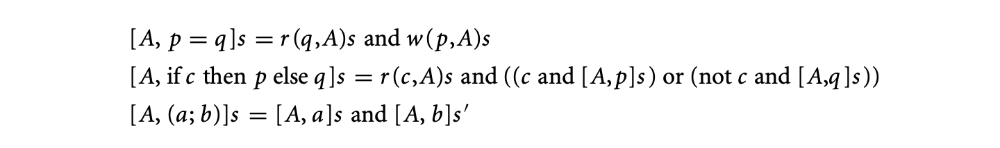 where is the new state after executing .
Here, can be a set of users also. Next, if , then can execute prog. The access control problem now becomes: Is there a program that can execute and that computes the value of some, forbidden, value and writes it to a location that can access? With HRU-type models, the set of programs to be examined is essentially unbounded, and we have undecidability. However, if we restrict the programs to be finite, decidability is possible.
It is also possible to model dynamic access control by other methods such as using pushdown systems [34], graph grammars [5], but we will only discuss the access control problem on the Internet that can be modeled using pushdown systems.
2.4.3 Retrofitting Simple MAC Models for SELinux
Since SELinux is easily available, we will use it as an example for discussing access control. In the past, the lack of such operating systems made research difficult; they were either classified or very expensive.
Any machine hosting some services on the net should not get totally compromised if there is a break-in. Can we isolate the breach to those services and not let it affect the rest of the system? It is possible to do so if we can use mandatory access policies (MACs) rather than the standard DACs. In a MAC the system decides how you share your objects, whereas in a DAC you can decide how you share your objects. A break-in into a DAC system has the potential to usurp the entire machine, whereas in a MAC system the kernel or the system still validates each access according to a policy loaded beforehand.
For example, in some recent Linux systems (e.g., Fedora Core 5/6, which is based on SELinux) that employ MAC, there is a "targeted" policy where every access to a resource is allowed implicitly, but deny rules can be used to prevent accesses. By default, most processes run in an "unconfined" domain, but certain daemons or processes7 (targeted ones) run in "locked-down" domains after starting out as unconfined. If cracker breaks into apache and gets a shell account, it can run only with the privileges of the locked-down daemon, and the rest of the system is usually safe. The rest of the system is not safe only if there is a way to effect a transition into the unconfined domain. With the more stringent "strict policy," also available in Fedora Core 5/6, that implicitly denies everything and "allow" rules are used to enable accesses, it is even more difficult.
httpd, dhcpd, mailman, mysqld, named, nscd, ntpd, portmap, postgresql, squid, syslogd, winbind, and snmpd.
Every subject (process) and object (e.g., file, socket, IPC object, etc.) has a security context that is interpreted only by a security server. Policy enforcement code typically handles security identifiers (SIDs); SIDs are nonpersistent and local identifiers. SELinux implements a combination of:
- Type enforcement and (optional) multilevel security: Typed models have been shown to be more tractable for analysis. Type enforcement requires that the type of domains and objects be respected when making transitions to other domains or when acting on objects of a certain type. It also offers some preliminary support for models that have information at different levels of security. The bulk of the rules in most policies in SELinux are for type enforcement.
- Role-based access control (RBAC): Roles for processes. Specifies domains that can be entered by each role and specifies roles that are authorized for each user with an initial domain associated with each user role. It has the ease of management of RBAC with fine granularity of type enforcement.
The security policy is specified through a set of configuration files.
However, one downside is that very fine level control is needed. Every major component such as NFS or X needs extensive work on what permissions need to be given before it can do its job. As the default assumption is "deny," there could be as many as 30,000 allow rules. There is a critical need for automated analysis. If the rules are too lax, we can have a security problem. If we have too few rules (too strict), a program can fail at runtime, as it does not have enough permissions to carry out its job. Just as in software testing, we need to do code coverage analysis. In the simplest case, without alias analysis or interprocedural analysis, it is possible to look at the static code and decide what objects are needed to be accessed. Assuming that all the paths are possible, one can use abstract interpretation or program slicing to determine the needed rules. However, these rules will necessarily be conservative. Without proper alias analysis in the presence of aliasing, we will have to be even more imprecise; similar is the case in the context of interprocedural analysis.
Ganapathy et al. [22] discuss automated authorization policy enforcement for user-space servers and the Linux kernel. Here, legacy code is retrofitted with calls to a reference monitor that checks permissions before granting access (MAC). For example, information "cut" from a sensitive window in an X server should not be allowed to be "pasted" into an ordinary one. Since manual placing of these calls is error prone, an automated analysis based on program analysis is useful. First, security-sensitive operations to be checked ("MACed") are identified. Next, for each such operation, the code-level constructs that must be executed are identified by a static analysis as a conjunction of several code-level patterns in terms of their ASTs. Next, locations where these constructs are potentially performed have to be located and, where possible, the "subject" and "object" identified. Next the server or kernel is instrumented with calls to a reference monitor with subject, object, and op triple as the argument, with a jump to the normal code on success or with call to a code that handles the failure case.
We now discuss the static analysis for automatic placement of authorization hooks, given, for example, the kernel code and the reference monitor code [21]. Assuming no recursion, the call graph of the reference monitor code is constructed. For each node in the call graph, a summary is produced. A summary of a function is the set of pairs that denotes the condition under which can be authorized by the function. For computing the summary, a flow and context-sensitive analysis is used that propagates a predicate through the statements of the function. For example, at a conditional statement with as the condition, the "if" part is analyzed with , and the "then" part by . At a call site, each pair in the summary of the function is substituted with the actuals of the call, and the propagation of the predicate continues. When it terminates, we have a set of pairs as summary. Another static analysis on the kernel source recovers the set of conceptual operations that may be performed by each kernel function. This is done by searching for combinations of code patterns in each kernel function. For each kernel function, it then searches through a set of idioms for these code patterns to determine if the function performs a conceptual operation; an idiom is a rule that relates a combination of code patterns to conceptual operations.
Once the summary of each function in the reference monitor code and the set of conceptual operations () for each kernel function is available, finding the set of functions in the monitor code that guards reduces to finding a cover for the set using the summary of functions .
Another tractable approach is for a less granular model but finer than non-MAC systems. For example, it is typically the case in a large system that there are definitely forbidden accesses and allowable accesses but also many "gray" areas. "Conflicting access control subspaces" [32] result if assignments of permissions and constraints that prohibit access to a subject or a role conflict. Analyzing these conflicts and resolving them, an iterative procedure, will result in a workable model.
2.4.4 Model Checking Access Control on the Internet: Trust Management
Access control is based on identity. However, on the Internet, there is usually no relationship between requestor and provider prior to request (though cookies are one mechanism used). When users are unknown, we need third-party input so that trust, delegation, and public keys can be negotiated. Withpublic key cryptography, it becomes possible to deal with anonymous users as long as they have a public key: authentication/authorization is now possible with models such as SPKI/SDSI (simple public key infrastructure/simple distributed security infrastructure) [15] or trust management. An issuer authorizes specific permissions to specific principals; these credentials can be signed by the issuer to avoid tampering. We can now have credentials (optionally with delegation) with the assumption that locally generated public keys do not collide with other locally generated public keys elsewhere. This allows us to exploit local namespaces: any local resource controlled by a principal can be given access permissions to others by signing this grant of permission using the public key.
We can now combine access control and cryptography into a larger framework with logics for authentication/authorization and access control. For example, an authorization certificate (K, S, D, T, V) in SPKI/SDSI can be viewed as an ACL entry, where keys or principals represented by the subject S are given permission, by a principal with public key K, to access a "local" resource T in the domain of the principal with public key K. Here, T is the set of authorizations (operations permitted on T), D is the delegation control (whether S can in turn give permissions to others), and V is the duration during which the certificate is valid.
Name certificates define the names available in an issuer's local namespace, whereas authorization certificates grant authorizations or delegate the ability to grant authorizations. A certificate chain provides proof that a client's public key is one of the keys that has been authorized to access a given resource either directly or transitively, via one or more name definition or authorization delegation steps. A set of SPKI/SDSI name and authorization certificates defines a pushdown system [34], and one can "model check" many of the properties in polynomial time. Queries in SPKI/SDSI [15] can be as follows:
- Authorized access: Given resource R and principal K, is K authorized to access R? Given resource R and name N (not necessarily a principal), is N authorized to access R? Given resource R, what names (not necessarily principals) are authorized to access R?
- Shared access: For two given resources R1 and R2, what principals can access both R1 and R2? For two given principals K1 and K2, what resources can be accessed by both K1 and K2?
- Compromisation assessment: Due (solely) to the presence of maliciously or accidentally issued certificate set C0 C, what resources could principal K have gained access to? What principals could have gained access to resource R?
- Expiration vulnerability: If certificate set C0 C expires, what resources will principal K be prevented from accessing? What principals will be excluded from accessing resource R?
- Universally guarded access: Is it the case that all authorizations that can be issued for a given resource R must involve a cert signed by principal K? Is it the case that all authorizations that grant a given principal K0 access to some resource must involve a cert signed by K?
Other models of trust management such as RBAC-based trust management (RT) [41] are also possible. The following rules are available in the base model RT[]:
- Simple member: . A asserts that D is a member of A's role.
- Simple inclusion: . This is delegation from A to B.
The model RT[] adds to RT[] the following intersection inclusion rule: and . This adds partial delegations from A to B1 and to B2. The model RT[] adds to RT[] the following linking inclusion rule: . This adds delegation from A to all the members of the role RT[] is all of the above four rules. The kinds of questions we would like to ask are:
- Simple safety (existential): Does a principal have access to some resource in some reachable state?
- Simple availability: In every state, does some principal have access to some resource?
- Bounded safety: In every state, is the number of principals that have access to some resource bounded?
- Liveness (existential): Is there a reachable state in which no principal has access to a given resource? Mutual exclusion: In every reachable state, are two given properties (or two given resources) mutually exclusive (i.e., no principal has both properties [or access to both resources] at the same time)?
- Containment: In every reachable state, does every principal that has one property (e.g., has access to a resource) also have another property (e.g., is an employee)? Containment can express safety or availability (e.g., by interchanging the two example properties in the previous sentence).
The complexity of queries such as simple safety, simple availability, bounded safety, liveness, and mutual exclusion analysis for is decidable in poly time in size of state. For containment analysis [41], it is P for , coNP-complete for , PSPACE-complete for , and decidable in coNEXP for .
However, permission-based trust management cannot easily authorize principals with a certain property. For example [41], to give a 20% discount to students of a particular institute, the bookstore can delegate discount permission to the institute key. The institute has to delegate its key to each student with respect to "bookstore" context; this can be too much burden on the institute. Alternatively, the institute can create a new group key for students and delegate it to each student key, but this requires that the institute create a key for each meaningful group; this is also too much burden. One answer to this problem is an attribute-based approach, which combines RBAC and trust management.
The requirements in an attribute-based system [40] are decentralization, provision of delegation of attribute authority, inference, attribute-based delegation of attribute authority, conjunction of attributes, attributes with fields (expiry, age, etc.) with the desirable features of expressive power, declarative semantics, and tractable compliance checking. Logic programming languages such as Prolog or, better, Datalog can be used for a delegation logic for ABAC: this combines logic programming with delegation and possibly with monotonic or nonmonotonic reasoning. With delegation depth and complex principals such as out of (static/dynamic) thresholds, many more realistic situations can be addressed.
Related to the idea of attribute-based access control and to allow for better interoperability across administrative boundaries of large systems, an interesting approach is the use of proof-carrying authentication [2]. An access is allowed if a proof can be constructed for an arbitrary access predicate by locating and using pieces of the security policy that have been distributed across arbitrary hosts. It has been implemented as modules that extend a standard web server and web browser to use proof-carrying authorization to control access to web pages. The web browser generates proofs mechanically by iteratively fetching proof components until a proof can be constructed. They provide for iterative authorization, by which a server can require a browser to prove a series of challenges.
2.5 Language-Based Security
As discussed earlier, current operating systems are much bigger than current compilers, so it is worthwhile to make the compiler part of the TCB rather than an OS. If it is possible to express security policies using a programming language that can be statically analyzed, a compiler as part of a TCB makes eminent sense.
The main goal of language-based security is to check the noninterference property, that is, to detect all possible leakages of some sensitive information through computation, timing channels, termination channels, I/O channels, and so on. However, the noninterference property is too restrictive to express security policies, since many programs do leak some information. For example, sensitive data after encryption can be leaked to the outside world, which is agreeable with respect to security as long as the encryption is effective. Hence, the noninterference property has to be relaxed by some mechanisms like declassification.
Note that static approaches cannot quantify the leakage of information, as the focus is on whether a program violated some desired property with respect to information flow. It is possible to use a dynamic approach that quantifies the amount of information leaked by a program as the entropy of the program's outputs as a distribution over the possible values of the secret inputs, with the public inputs held constant [43]. Noninterference has an entropy of 0. Such a quantitative approach will often be more useful and flexible than a strict static analysis approach, except that analysis has to be repeated multiple times for coverage.
One approach to static analysis for language-based security has been to use type inference techniques, which we discuss next.
2.5.1 The Type-Based Approach
Type systems establish safety properties (invariants) that hold throughout the program, whereas noninterference requires that two programs give the same output in spite of different input values for their "low" values. Hence, a noninterference proof can be viewed as a bisimulation. For simpler languages (discussed below), a direct proof is possible, but for languages with advanced features such as concurrency and dynamic memory allocation, noninterference proofs are more complex. Before we proceed to discuss the type-based approach, we will briefly describe the lattice model of information flow.
The lattice model of information flow started with the work of Bell and LaPadula [6] and Denning and Denning [17]. Every program variable has a static security class (or label); the security label of each variable can be global (as in early work) or local for each owner, as in the decentralized label model (DLM) developed for Java in Jif [45].
If and are variables, and there is (direct) information flow from to , it is permissible iff the label of is less than that of . Indirect flows arise from control flow such as if (y=1) then x=1 else x=2. If the label of the label of , some information of flows into (based on whether is 1 or 2) and should be disallowed. Similarly, if (y=z) then x=1 else w=2, the of the levels of and should be of the levels of and . To handle this situation, we can assign a label to the program counter (). In the above example, we can assign the label of the to just after evaluating the condition; the condition now that needs to be satisfied is that both the arms of the if should have at least the same level as the .
Dynamic labels are also possible. A method may take parameters, and the label of the parameter itself could be an another formal. In addition, array elements could have different labels based on index, and hence an expression could have a dynamic label based on the runtime value of its index.
Checking that the static label of an expression is at least as restrictive as the dynamic label of any value it might produce is now one goal of analysis (preferably static). Similarly, in the absence of declassification, we need to check that the static label of a value is at least as restrictive as the dynamic label of any value that might affect it. Because of the limitations of analysis, static checking may need to use conservative approximations for tractability.
Denning and Denning proposed program certification as a lattice-based static analysis method [17] to verify secure information flow. However, soundness of the analysis was not addressed. Later work such as that of Volpano and colleagues [55] showed that a program is secure if it is "typable," with the "types" being labels from a security lattice. Upward flows are handled through subtyping. In addition to checking correctness of flows, it is possible to use type inference to reduce the need to annotate the security levels by the programmer. Type inference computes the type of any expression or program. By introducing type variables, a program can be checked if it can be typed by solving the constraint equations (inequalities) induced by the program. In general, simple type inference is equivalent to first-order unification, whereas in the context of dependent types it is equivalent to higher-order unification.
For example, consider a simple imperative language with the following syntax [55]:
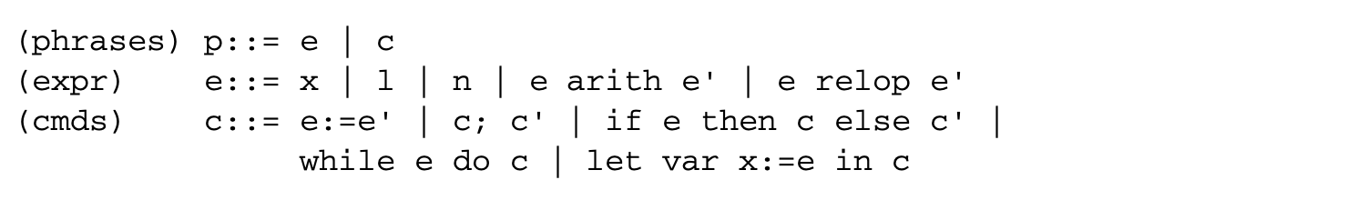
Here, l denotes locations (i.e., program counter values), n integers, x variables, and c constants. The types in this system are types of variables, locations, expressions, and commands; these are given by one of the partially ordered security labels of the security system. A cmd has a type only if it is guaranteedthat every assignment in cmd is made to a variable whose security class is t or higher. The type system for security analysis is as follows ( and are location and type environments, respectively):
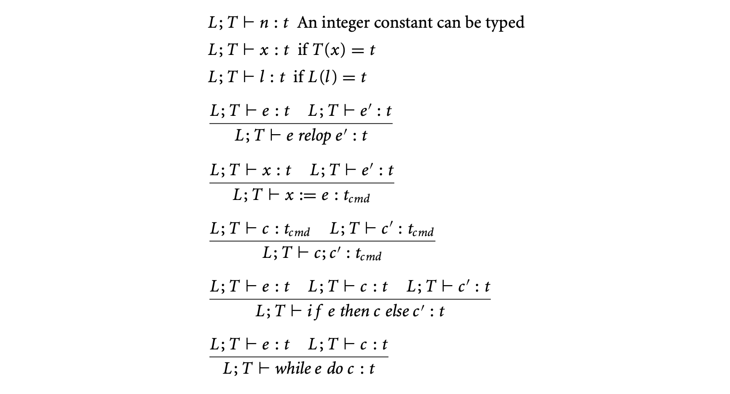
Consider the rules for assignment above. In order for information to flow from to , both have to be at the same security level. However, upward flow is allowed, for secrecy, for example, if is at a higher level and is at a lower level. This is handled by extending the partial order by subtyping and coercion: the low level (derived type) is smaller (for secrecy) in this extended order than the high level (base type). Note that the extended relation has to be contravariant in the types of commands .
It can be proved [55] that if an expression can be given a type in the above type system, then, for secrecy, only variables at level or lower in will have their contents read when is evaluated (no read up). For integrity, every variable in stores information at integrity level . If a command has the property that every assignment within is made to a variable whose security class is at least , then the confinement property for secrecy says that no variable below level is updated in (no write down). For integrity, every variable assigned in can be updated by a type variable.
Soundness of the type system induces the noninterference property, that is, a high value cannot influence any lower value (or information does not leak from high values to low values).
Smith and Volpano [53] have studied information flow in multithreaded programs. The above type system does not guarantee noninterference; however, by restricting the label of all the while-loops and its guards to low, the property is restored. Abadi has modeled encryption as declassification [1] and presented the resulting type system.
Myers and colleagues have developed static checking for DLM-based Jif language [12, 16], while Pottier and colleagues [49] have developed OCaml-based FlowCAML. We discuss the Jif approach in some detail.
2.5.2 Java Information Flow (Jif) Language
Jif is a Java-based information flow programming language that adds static analysis of information flow for improved security assurance. Jif is mainly based on static type checking. Jif also performs some runtime information flow checks.
Jif is based on decentralized labels. A label in Jif defines the security level, represented by a set of policy expressions separated by semicolons. A policy expression means the principal owner wants to allow labeled information to flow to at most the principal's reader. Unlike the MAC model, these labels contain fine-grained policies, which have an advantage of being able to represent decentralized access control. These labels are called decentralized labels because they enforce security on behalf of the owning principals, not on behalf of an implicitly centralized policy specifier. The policy specifies that both and own the information with each allowing either or , respectively. For integrity, another notation is adopted.
Information can flow from label to label only if (i.e., is less restrictive than ), where defines a preorder on labels in which the equivalence classes form a join semilattice. To label an expression (such as ), a join operator is defined as the lub of the labels of the operands, as it has to have a secrecy as strong as any of them. In the context of control flow, such as if cond then x=... else x=..., we also need the join operator. To handle implicit flows through control flow, each program visible location is given an implicit label.
A principal hierarchy allows one principal to actfor another. This helps in simplifying the policy statements in terms of representation of groups or roles. For example, suppose principal Alice actsfor Adm and principal Bob actsfor Adm; thus, in the following code whatever value Adm has is also readable by Alice and Bob.
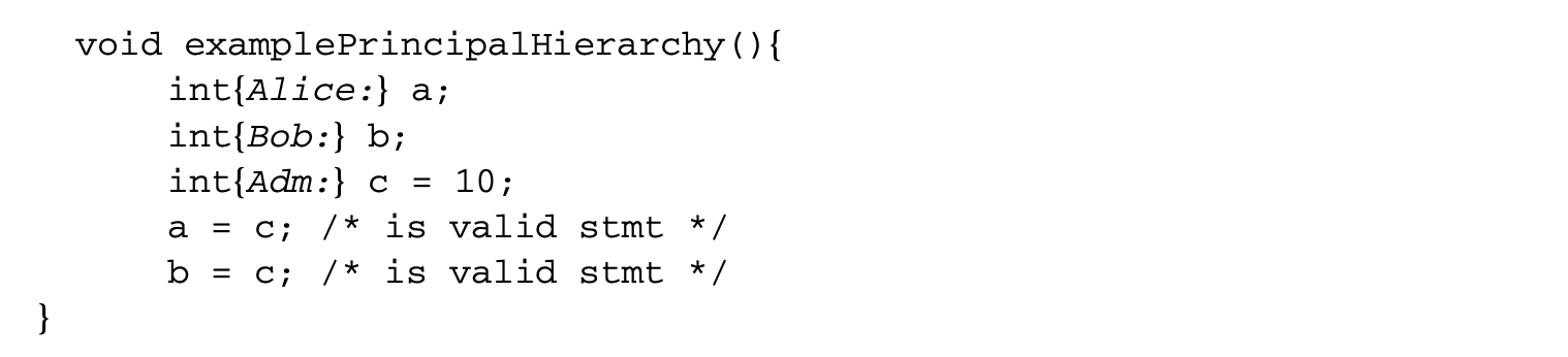
The declassification mechanism gives the programmer an explicit escape hatch for releasing information whenever necessary. The declassification is basically carried out by relaxing the policies of some labels by principals having sufficient authority. For example,

Jif has label polymorphism. This allows the expression of code that is generic with respect to the security class of the data it manipulates. For example,
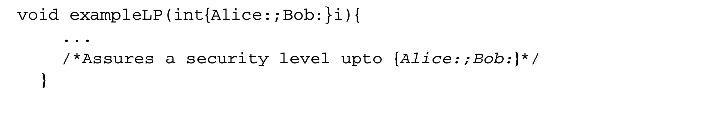
To the above function (which assures a security level up to {Alice;Bob:}) one can pass any integer variable having one of the following labels:
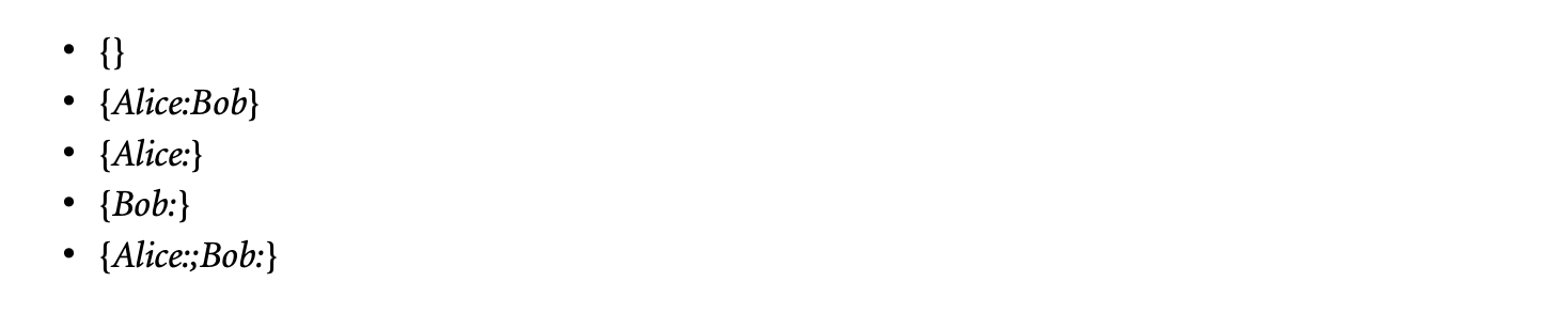
Jif has automatic label inference. This makes it unnecessary to write many type-annotations. For example, suppose the following function is called (which can only be called from a program point with label at most {Alice;Bob:}) from a valid program point; "a" will get a default label of {Alice;Bob:}.
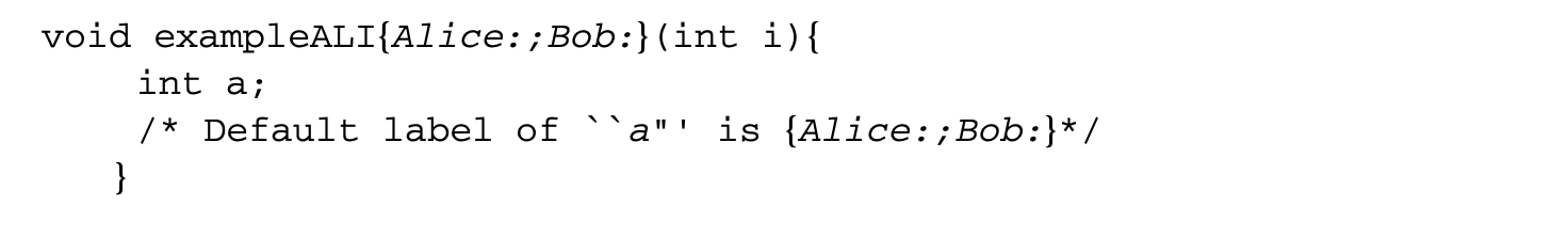
Runtime label checking and first-class label values in Jif make it possible to discover and define new policies at runtime. Runtime checks are statically checked to ensure that information is not leaked by the success or failure of the runtime check itself. Jif provides a mechanism for comparing runtime labels and also a mechanism for comparing runtime principals. For example,
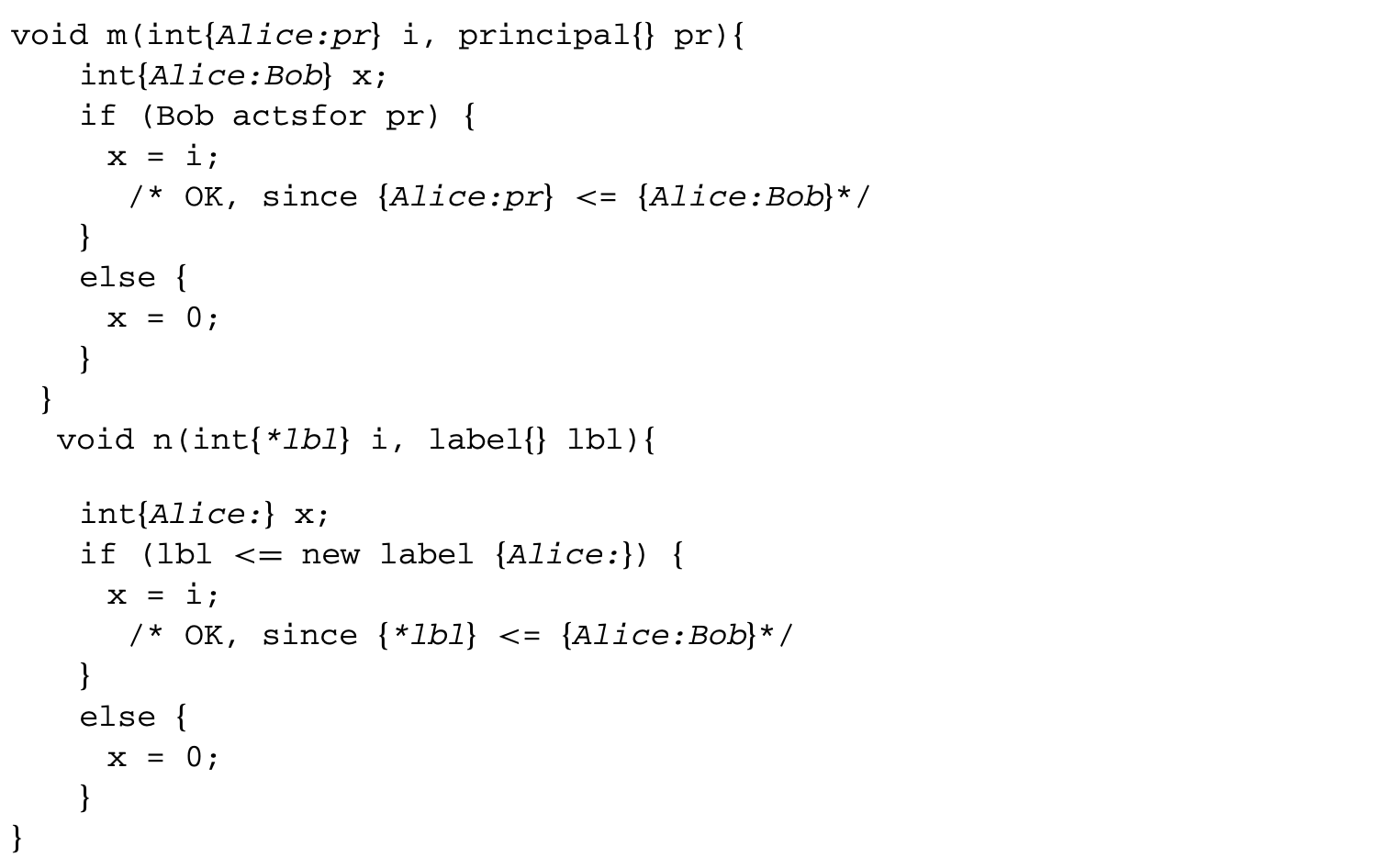
Note that in the above function n(...), "lbl represents an actual label held by the variable lbl, whereas just lbl inside a label represents the label of the variable lbl (i.e., {} here).
Labels and principals can be used as first-class values represented at runtime. These dynamic labels and principals can be used in the specification of other labels and used as the parameters of parameterized classes. Thus, Jif's type system has dependent types. For example,

Note that, unlike in Java, method arguments in Jif are always implicitly final. Some of the limitations of Jif are that there is no support for Java Threads, nested classes, initializer blocks, or native methods.
Interaction of Jif with existing Java classes is possible by generating Jif signatures for the interface corresponding to these Java classes.
2.5.3 A Case Study: VSR
The context of this section8 is the security of archival storage. The central objective usually is to guarantee the availability, integrity, and secrecy of a piece of data at the same time. Availability is usually achieved through redundancy, which reduces secrecy (it is sufficient for the adversary to get one copy of the secret). Although the requirements of availability and secrecy seem to be in conflict, an information-theoretic secret sharing protocol was proposed by Shamir in 1979 [51], but this algorithm does not provide data integrity. Loss of shares can be tolerated up to a threshold but not to arbitrary modifications of shares.
This is joint work with a former student, S. Roopesh.
A series of improvements have therefore been proposed over time to build secret sharing protocols resistant to many kinds of attacks. The first one takes into account the data-integrity requirement and leads to verifiable secret sharing (VSS) algorithms [20, 48]. The next step is to take into account mobile adversaries that can corrupt any number of parties given sufficient time. It is difficult to limit the number of corrupted parties on the large timescales over which archival systems are expected to operate. An adversary can corrupt a party, but redistribution can make that party whole again (in practice, this happens, for example, following a system re-installation). Mobile adversaries can be tackled by means of proactive secret sharing (PSS), wherein redistributions are performed periodically. In one approach, the secret is reconstructed and then redistributed. However, this causes extra vulnerability at the node of reconstruction. Therefore, another approach, redistribution without reconstruction, is used [33]. A combination of VSS and PSS is verifiable secret redistribution (VSR); one such protocol is proposed in [58]. In [26] we proposed an improvement of this protocol, relaxing some of the requirements.
Modeling the above protocol using Jif can help us understand the potential and the difficulties of Jif static analysis. We now discuss the design of a simplified VSR [58] protocol:
-
Global values: This class contains the following variables that are used for generation and verification of shares and subshares during reconstruction and redistribution phases. (m,n): is the threshold number of servers required for reconstruction of a secret, and is the total number of servers to which shares are distributed. p: The prime used for ; is the prime used for . g: The Diffie-Hellman exponentiator. KeyID: Unique for each secret across all clients. ClientID: ID of the owner of the secret.
-
Secret: This class contains secret's value (i.e., the secret itself), the polynomial used for distribution of shares, N[] -- the array of server IDs to which the shares are distributed.
-
Points2D: This class contains two values x and f(x), where is the polynomial used for generating the shares (or subshares). It is used by Lagrangian interpolator to reconstruct the secret (or shares from subshares).
-
Share: This class contains an immutable original share value (used to check whether shares are uncorrupted or not) and a redistributing polynomial (used for redistribution of this share to a new access structure).
-
SubShare: This is the same as the Share class, except that the share value actually contains a subshare value and no redistributing polynomial.
-
SubShareBox: This class keeps track of the subshares from a set of valid servers (i.e., B[] servers) in the redistribution phase. This is maintained by all servers belonging to the new (m,n)-access structure to which new shares are redistributed.
-
Client: This class contains zero or more secrets and is responsible for initial distribution of shares and reconstruction of secrets from valid sets of servers.
-
Server: This class maintains zero or more shares from different clients and is responsible for redistribution of shares after the client (who is the owner of the secret corresponding to this share) has approved the redistribution.
-
Node: Each node contains two units, one Client and the other Server (having the same IDs as this node). On message reception from the reliable communication (group communication system [GCS]) interface GCSInterface, this node extracts the information inside the message and gives it to either the client or the server, based on the message type.
-
GCSInterface: This communication interface class is responsible for acting as an interface between underlying reliable messaging systems (e.g., the Ensemble GCS [30] system), user requests, and Client and Server.
-
UserCommand (Thread): This handles three types of commands from the user: Distribution of the user's secret to (m,n)-access structure Redistribution from (m,n)-access structure Reconstruction of secret
-
SendMessage (Thread): This class packetizes the messages (from Node) (depends on the communication interface), then either sends or multicasts these packets to the destination node(s).
-
Attacker: This class is responsible for attacking the servers, getting their shares, and corrupting all their valid shares (i.e., changing the values in the Points2D class to arbitrary values). This class also keeps all valid shares it got by attacking the servers. It also reconstructs all possible secrets from the shares collected. Without loss of generality, we assume that at most one attacker can be running in the whole system.
-
AttackerNode: This is similar to Node, but instead of Client and Server instances, it contains only one instance of the Attacker class.
-
AttackerGCSInterface: Similar to the GCSInterface class.
-
AttackerUserCommand: This handles two types of commands from the attacker: Attack server S Construct all possible secrets from collected valid shares
We do not dwell on some internal bookkeeping details during redistribution and reconstruction phases. Figure 2.1 gives the three phases of the simplified VSR protocol. The distribution and reconstruction phases almost remain the same. Only the redistribution phase is slightly modified, where the client acts as the manager of the redistribution process. The following additional assumptions are also made:
-
There are no "Abort" or "Commit" messages from servers.
-
In the redistribution phase, the client, who is the owner of the secret corresponding to this redistribution process, will send the "commit" messages instead of the redistributing servers.
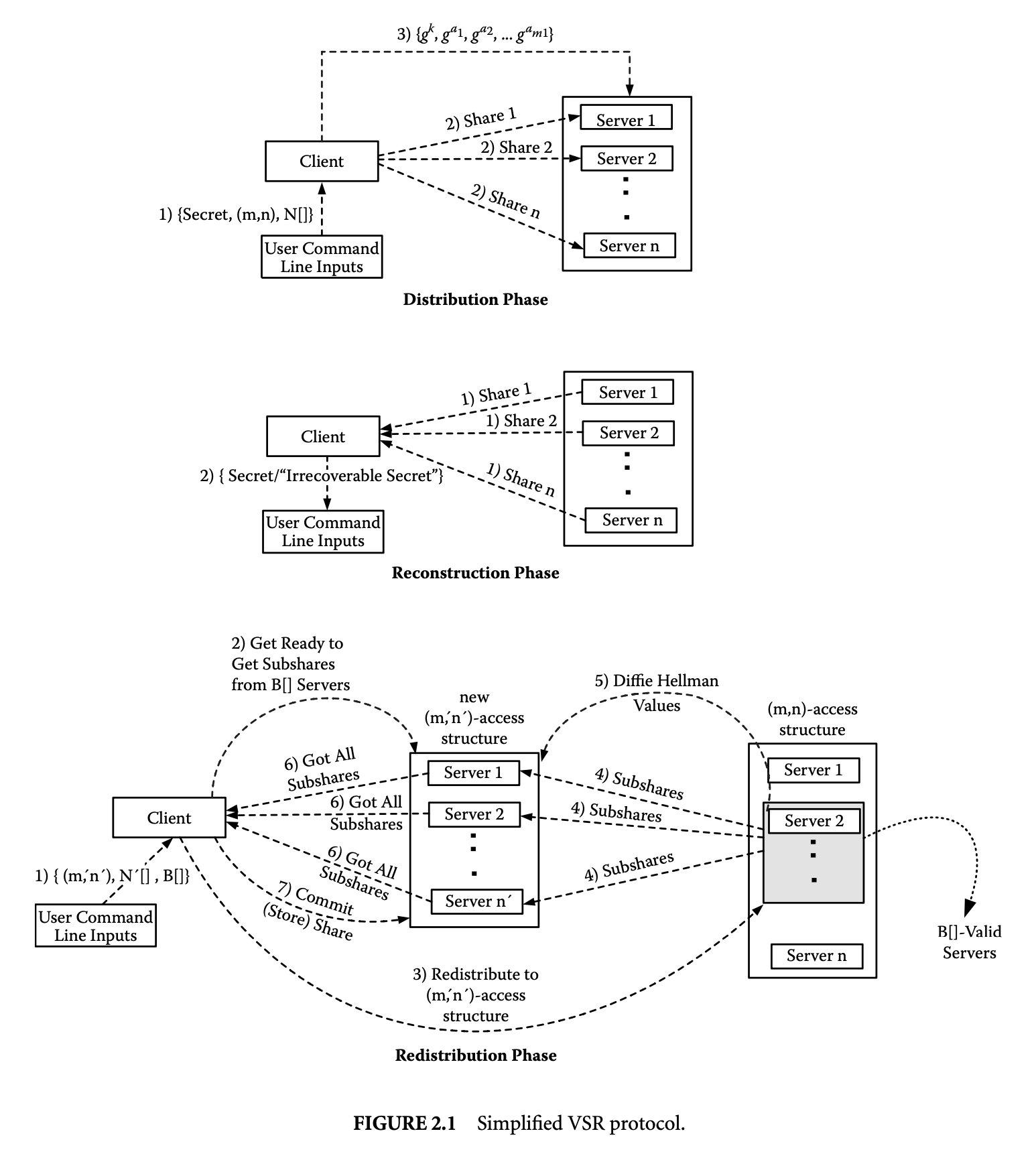
-
Attacker is restricted to only attacking the servers and thereby getting all the original shares, which are held by the servers, and corrupting them.
-
There are no "reply and DoS attacks" messages.
2.5.3.1 Jif Analysis of Simplified VSR
In this section, we discuss an attempt to do a Jif analysis on a simplified VSR implementation and its difficulties. As shown in Figure 2.2, every Node (including the AttakerNode) runs with "root" authority (who is above all and can actfor all principals). Every message from and out of the network will have an empty label (as we rely on underlying Java Ensemble for cryptographically perfect end-to-end and multicast communication). The root (i.e., Node) receives the message from the network. Based on the message type,
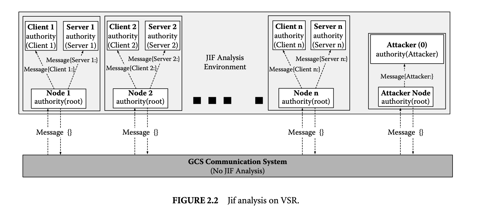
root will appropriately (classify or) declassify the contents of the message and handles them by giving them to either the client or server. Similarly, all outgoing messages from Client/Server to communication network would be properly declassified.
First, the communication interface (Java Ensemble) uses some native methods to contact ensemble-server.9 To do asynchronous communication we use threads in our VSR implementation. Since Jif does not support Java Threads and native methods, Jif analysis cannot be done at this level. Hence, we have to restrict the Jif analysis above the communication layer.10
ensemble-server is a daemon serving group communication.
Because of this separation, we encounter a problem with the Jif analysis even if we want to abstract out the lower GCS layer. Some of the classes (such as the Message class) are common to both upper and lower layers, but they are compiled by two different compilers (Jif and Java) that turn out to have incompatible .class files for the common classes.
Next, let us proceed to do static analysis on the remaining part using the Jif compiler. Consider the Attacker Node (see Figure 2.2). The attacker node (running with root authority) classifies all content going to the principal Attacker with the label-Attacker :. If the attacker has compromised some server, it would get all the valid shares belonging to that server. Hence, all shares of a compromised server output from the communication interface (GCS) go to the attacker node first. Since it is running with root authority and sees that shares are semi-sensitive, it (de)classifies these shares to {Server:}. For these shares to be read by the attacker, the following property should hold: {Server:} {Attacker:}.
However, since the Attacker principal does not actsfor this Server (principal), the above relation does not hold, so the attacker cannot read the shares. The Jif compiler detected this as an error. However, if we add an actsfor relation from Attacker (principal) to this Server (principal) (i.e., Attacker actsfor Server), it could read the shares. In this case, the Jif compiler does not report any error, implying that the information flow from {Server:} to {Attacker:} is valid (since {Server:} {Attacker:} condition holds).
VSR has a threshold property: if the number of shares (or subshares) is more than the threshold, the secret can be reconstituted. This implies that any computation knowing less than the threshold number of shares cannot interfere with any computation that has access to more than this threshold. We need a threshold set noninterference property. This implies that we can at most declassify less than any set of a threshold number of shares. Since such notions are not expressible in Jif, even if mathematically proved as in [58], more powerful dependent-type systems have to be used in the analysis. Since modern type inference is based on explicit constraint generation and solving, it is possible to model the threshold property through constraints, but solving such constraints will have a high complexity. Fundamentally, we have to express the property that any combination of subshares less than the threshold number cannot
interfer (given that the number of subshares available is more than this number); either every case has to be discharged separately or symmetry arguments have to be used. Approaches such as model checking (possibly augmented with symmetry-based techniques) are indicated.
There is also a difficulty in Jif in labeling each array element with different values. In the Client class, there is a function that calculates and returns the shares of a secret. Its skeleton code is as follows:
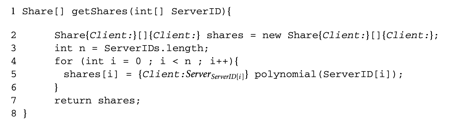
In line 2, "shares" is an array of type "Share" with a label of [Client:] for both array variable and individual elements of this array. Line 5 calculates different shares for different servers based on ServerIDs and assigns a different label of {Client:ServerServerID[i]} for each of these shares. However, Jif does not allow for different labels for different elements of an array; it only allows a common label for all elements of an array. If this is possible, we should ensure that accessing some array element does not itself leak some information about the index value.
There are currently many other difficulties in using Jif to do analysis such as the need to recode a program in Jif. The basic problem is the (post hoc) analysis after an algorithm has already been designed. What is likely to be more useful11 is an explicit security policy before the code is developed [60] and then use of Jif or a similar language to express and check these properties where possible. McCamant and Ernst [43] argue that Jif-type static analysis is still relatively rare and no "large" programs have yet been ported to Jif or FlowCaml. They instead use a fine-grained dynamic bit-tracking analysis to measure the information revealed during a particular execution.
In the verification area, it is increasingly becoming clear that checking the correctness of finished code is an order of magnitude more difficult than intervening in the early phases of the design.
2.6 Future Work
Current frameworks such as Jif have not been sufficiently developed. We foresee the following evolution:
- The analysis in Section 2.5.1 assumed that typing can reveal interesting properties. This needs to be extended to a more general static analysis that deals with values in addition to types as well as when the language is extended to include arrays and so on. Essentially, the analysis should be able to handle array types with affine index functions. This goes beyond the analysis possible with type analysis.
- Incorporate pointers and heaps in the analysis. Use dataflow analysis on lattices but with complex lattice values (such as regular expressions, etc.) or use shape analysis techniques.
- Integrate static analysis (such as abstract interpretation and compiler dataflow analysis) with model checking to answer questions such as: What is the least/most privilege a variable should have to satisfy some constraint? This may be coupled with techniques such as counterexample guided abstraction refinement [13]. This, however, requires considerable machinery. Consider, for example, a fully developed system such as the SLAM software model checking [3]. It uses counterexample-drivenabstraction of software through "boolean" programs (or abstracted programs) using model creation (c2bp), model checking (bebop), and model refinement (newton). SLAM builds on the OCaml programming language and uses dataflow and pointer analysis, predicate abstraction and symbolic model checking, and tools such as CUDD, a SAT solver, and an SMT theorem prover [3]. Many such analyses have to be developed for static analysis of security properties.
References
[1] Martin Abadi. Secrecy by Typing in Security Protocols. TACS 1997.
[2] Andrew W. Appel and Edward W. Felten. 1999. Proof-carrying authentication. Proceedings of the 6th ACM Conference on Computer and Communications Security, 52-62. New York: ACM Press.
[3] Thomas Ball and Sriram K. Rajamani. 2002. The SLAM project: debugging system software via static analysis. In Proceedings of the 29th ACM SIGPLAN-SIGACT Symposium on Principles of Programming Languages, 1-3.
[4] B. Barak, O. Goldreich, R. Impagliazzo, S. Rudich, A. Sahai, S. Vadhan, and K. Yang. 2001. On the (im)possibility of obfuscating programs. In Advances in cryptology (CRYPTO'01). Vol. 2139 of Lecture notes in computer science, 1-18, New York: Springer.
[5] Jorg Bauer, Ina Schaefer, Tobe Toben, and Bernd Westphal. 2006. Specification and verification of dynamic communication systems. In Proceedings of the Sixth International Conference on Application of Concurrency to System Design, 189-200. Washington, DC: IEEE Computer Society.
[6] D. Elliott Bell and Leonard J. LaPadula. 1973. Secure computer systems: Mathematical foundations. MITRE Corporation.
[7] Matt Bishop. 2002. Computer security: Art and science. Reading, MA: Addison-Wesley.
[8] R. Canetti. 2001. Universally composable security: A new paradigm for cryptographic protocols. 42nd FOCS, 2001. Revised version (2005). Online: http://eprint.iacr.org/2000/067
[9] Bryan M. Cantrill, Michael W. Shapiro, and Adam H. Leventhal. 2004. Dynamic instrumentation of production systems. In Proceedings of the 2004 USENIX Annual Technical Conference.
[10] Hao Chen, David Wagner, and Drew Dean. 2002. Setuid demystified. In Proceedings of the 11th USENIX Security Symposium, 171-90. Berkeley, CA: USENIX Assoc.
[11] David M. Chess and Steve R. White. 2000. An undetectable computer virus. Virus Bulletin Conference.
[12] S. Chong, A. C. Myers, K. Vikram, and L. Zheng. Jif reference manual. http://www.cs.cornell.edu/jif/doc/jif-3.0.0/manual.html.
[13] Edmund M. Clarke, Orna Grumberg, Somesh Jha, Yuan Lu, and Helmut Veith. 2000. Counterexample-guided abstraction refinement. In Proceedings of the 12th International Conference on Computer Aided Verification, 154-69. London: Springer Verlag.
[14] Edmund M. Clarke, Orna Grumberg, and Doron A. Peled. 2000. Model checking. Cambridge, MA: MIT Press.
[15] P. Clarke, J. E. Elien, C. Ellison, M. Fridette, A. Morcos, and R. L. Rivest. 2001. Certificate chain discovery in SPKI? SDSI. J. Comp. Security 9:285-332.
[16] Fred Cohen. 1987. Computer viruses: Theory and experiments. Comp. Security 6, Vol 6(1), pp. 22-35.
[17] Dorothy E. Denning and Peter J. Denning. 1977. Certification of programs for secure information flow. Commun. ACM 20(7):504-13.
[18] D. Dougherty, K. Fisler, and S. Krishnamurthi. 2006. Specifying and reasoning about dynamic access-control policies. International Joint Conference on Automated Reasoning (IJCAR), August 2006.
[19] Dawson Engler, Benjamin Chelf, Andy Chou, and Seth Hallem. Checking system rules using system-specific, programmer-written compiler extensions. In Proceedings of the 4th Symposium on Operating System Design and Implementation, San Diego, CA, October 2000.
[20] P. Feldman. 1987. A practical scheme for non-interactive verifiable secret sharing. In Proceedings of the 28th IEEE Annual Symposium on Foundations of Computer Science, 427-37.
[21] Vinod Ganapathy, Trent Jaeger, and Somesh Jha. 2005. Automatic placement of authorization hooks in the Linux security modules framework. In Proceedings of the 12th ACM Conference on Computer and Communications Security, 330-39. New York: ACM Press.
[22] Vinod Ganapathy, Trent Jaeger, and Somesh Jha. 2006. Retrofitting legacy code for authorization policy enforcement. Proceedings of the 2006 Symposium on Security and Privacy, 214-29. Washington, DC: IEEE Computer Society.
[23] V. Ganapathy, S. Jha, D. Chandler, D. Melski, and D. Vitek. 2003. Buffer overrun detection using linear programming and static analysis. In Proceedings of the 10th ACM Conference on Computer and Communications Security (CCS), 345-54. New York: ACM Press.
[24] Joseph A. Goguen and Jos Meseguer. 1982. Security policies and security models. In Proceedings of the 1982 IEEE Symposium on Security and Privacy, 11-20. Los Alamitos, CA: CS Press.
[25] Mohamed G. Gouda and Alex X. Liu. 2004. Firewall design: Consistency, completeness, and compactness. In Proceedings of the 24th International Conference on Distributed Computing Systems, 320-27. Washington, DC: IEEE Computer Society.
[26] V. H. Gupta and K. Gopinath. 2006. An extended verifiable secret redistribution protocol for archival systems. In International Conference on Availability, Reliability and Security, 100-107. Los Alamitos, CA: IEEE Computer Society.
[27] Joshua D. Guttman, Amy L. Herzog, and John D. Ramsdel. 2003. Information flow in operating Systems: Eager formal methods. WITS2003.
[28] K. W. Hamlen, Greg Morrisett, and F. B. Schneider. 2005. Computability classes for enforcement mechanisms. ACM TOPLAS 28:175-205.
[29] M. A. Harrison, W. L. Ruzzo, and J. D. Ullman. 1976. Protection in operating systems. Commun. ACM 19:461-71.
[30] Mark Hayden and Ohad Rodeh. 2004. Ensemble reference manual. Available online: http://dsl.cs. technion.ac.il/projects/Ensemble/doc/ref.pdf
[31] Trent Jaeger, Reiner Sailer, and Xiaolan Zhang. 2003. Analyzing integrity protection in the SELinux example policy. In Proceedings of the 11th USENIX Security Symposium. USENIX.
[32] Trent Jaeger, Xiaolan Zhang, and Fidel Cacheda. 2003. Policy management using access control spaces. ACM Trans. Inf. Syst. Security. 6(3):327-64.
[33] Sushil Jajodia and Yvo Desmedt. 1997. Redistributing secret shares to new access structures and its applications. Tech. Rep. ISSE TR-97-01, George Mason University.
[34] S. Jha and T. Reps. 2002. Analysis of SPKI/SDSI certificates using model checking. In Proceedings of the 15th IEEE Workshop on Computer Security Foundations, 129. Washington, DC: IEEE Computer Society.
[35] Jif: Java + information flow. <www.cs.cornell.edu/jif/>.
[36] R. B. Keskar and R. Venugopal. 2002. Compiling safe mobile code. In The compiler design handbook. Boca Raton, FL: CRC Press.
[37] M. Koch, L. V. Mancini, and F. Parisi-Presicce. 2002. Decidability of safety in graph-based models for access control. In Proceedings of the 7th European Symposium on Research in Computer Security, 229-43. London: Springer-Verlag.
[38] Butler W. Lampson. 1973. A note on the confinement problem. Commun. ACM 16(10):613-15.
[39] Felix Lazebnik. 1996. On systems of linear Diophantine equations. Math. Mag. 69(4).
[40] N. Li, B. N. Grosof, and J. Feigenbaum. 2003. Delegation logic: A logic-based approach to distributed authorization. ACM Trans. Inf. Syst. Security 6:128-171.
[41] Ninghui Li, John C. Mitchell, and William H. Winsborough. 2005. Beyond proof-of-compliance: Security analysis in trust management. J. ACM 52:474-514.
[42] Ninghui Li and Mahesh V. Tripunitara. 2005. Safety in discretionary access control. In Proceedings of the 2005 IEEE Symposium on Security and Privacy, 96-109. Washington, DC: IEEE Computer Society.
[43] Stephen McCamant and Michael D. Ernst. 2006. Quantitative information-flow tracking for C and related languages. MIT Computer Science and Artificial Intelligence Laboratory Tech. Rep. MIT-CSAIL-TB-2006-076, Cambridge, MA.
[44] Steven McCanne and Van Jacobson. 1993. The BSD packet filter: A new architecture for user-level packet capture. In Proceedings of the Winter Usenix Technical Conference, 259-69.
[45] Andrew C. Meyers. 1999. Mostly-static decentralized information flow control. MIT Laboratory for Computer Science, Cambridge, MA.
[46] George C. Necula, Scott McPeak, and Westley Weimer. 2002. CCured: Type-safe retrofitting of legacy code. In Annual Symposium on Principles of Programming Languages, 128-39. New York: ACM Press.
[47] Seth Nielson, Seth J. Fogarty, and Dan S. Wallach. 2004. Attacks on Local Searching Tools. Tech. Rep. TR04-445, Department of Computer Science, Rice University, Honston, TX.
[48] T. P. Pedersen. 1991. Non-interactive and information theoretic secure verifiable secret sharing. In Proceedings of CRYPTO 1991, the 11th Annual International Cryptology Conference, 129-40. London: Springer Verlag.
[49] Francois Pottier and Vincent Simonet. 2003. Information flow inference for ML. ACM Transac. Programming Languages Syst. 25(1):117-58.
[50] J. Rao, P. Rohatgi, H. Scherzer, and S. Tinguely. 2002. Partitioning attacks: Or how to rapidly clone some GSM cards. In Proceedings of the 2002 IEEE Symposium on Security and Privacy, 31. Washington, DC: IEEE Computer Society.
[51] A. Shamir. 1979. How to share a secret. Commun. ACM, 22(11):612-13.
[52] Geoffrey Smith and Dennis M. Volpano. 1998. Secure information flow in a multi-threaded imperative language. In Proceedings of the 25th ACM SIGPLAN-SIGACT Symposium on Principles of Programming Languages, 355-64. New York: ACM Press.
[53] Ken Thompson. 1984. Reflections on trusting trust. Commun. ACM, 27(8): 761-63.
[54] M. Y. Vardi. 1982. The complexity of relational query languages (extended abstract). In Proceedings of the 14th Annual Symposium on the Theory of Computing, 137-46. New York: ACM Press.
[55] Dennis M. Volpano, Cynthia E. Irvine, and Geoffrey Smith. 1996. A sound type system for secure flow analysis. J. Comput. Security 4(2/3):167-88.
[56] D. Wagner, J. Foster, E. Brewer, and A. Aiken. 2000. A first step towards automated detection of buffer overrun vulnerabilities. In Symposium on Network and Distributed Systems Security (NDSS00), February 2000, San Diego, CA.
[57] Wlikipedia. Trusted Computer System evaluation criteria. http://en.wikipedia.org/wiki/Trusted_Computer_System_Evaluation.
[58] Theodore M. Wong, Chenxi Wang, and Jeannette M. Wing. 2002. Verifiable secret redistribution for archival systems. In Proceedings of the First IEEE Security in Storage Workshop, 94. Washington, DC: IEEE Computer Society.
[59] Steve Zdancewic and Andrew C. Myers. 2001. Robust declassification. In Proceedings of the 2001 IEEE Computer Security Foundations Workshop.
[60] Steve Zdancewic, Lantian Zheng, Nathaniel Nystrom, and Andrew C. Myers. 2001. Untrusted hosts and confidentiality: Secure program partitioning. In ACM Symposium on Operating Systems Principles. New York: ACM Press.
3. Compiler-Aided Design of Embedded Computers
3.1 Introduction
Embedded systems are computing platforms that are used inside a product whose main function is different than general-purpose computing. Cell phones and multipoint fuel injection systems in cars are examples of embedded systems. Embedded systems are characterized by application-specific and multidimensional design constraints. While decreasing time to market and the need for frequent upgrades are pushing embedded system designs toward programmable implementations, these stringent requirements demand that designs be highly customized. To customize embedded systems, standard design features of general-purpose processors are often omitted, and several new features are introduced in embedded systems to meet all the design constraints simultaneously.
Consequently, software development for embedded systems has become a very challenging task. Traditionally humans used to code for embedded systems directly in assembly language, but now with the software content reaching multimillion lines of code and increasing at the rate of 100 times every decade, compilers have the onus of generating code for embedded systems. With embedded system designs still being manually customized, compilers have a dual responsibility: first to exploit the novel architectural features in the embedded systems, and second to avoid the loss due to missing standard architectural features. Existing compiler technology falls tragically short of these goals.
While the task of the compiler is challenging in embedded systems, it has been shown time and again that whenever possible, a compiler can have a very significant impact on the power, performance, and so on of the embedded system. Given that the compiler can have a very significant impact on the design constraints of embedded systems. Consequently, it is only logical to include the compiler during the design of the embedded system. Existing embedded system design techniques do not include the compiler during the design space exploration. While it is possible to use ad hoc methods to include the compiler's effects during the design of a processor, a systematic methodology to perform compiler-aware embedded systems design is needed. Such design techniques are called compiler-aided design techniques.
This chapter introduces our compiler-in-the-loop (CIL) design methodology, which systematically includes compiler effects to design embedded processors. The core capability in this methodology is a design space exploration (DSE) compiler. A DSE compiler is different from a normal compiler in that a DSE compiler has heuristics that are parameterized on the architectural parameters of the processor architecture. While typical compilers are built for one microarchitecture, a DSE compiler can generate good-quality code for a range of architectures. A DSE compiler takes the architecture description of the processor as an input, along with the application source code, and generates an optimized executable of the application for the architecture described.
The rest of the chapter is organized as follows. In Section 3.2, we describe our whole approach of using a compiler for processor design. In particular, we attempt to design the popular architectural feature, in embedded processors, called horizontally partitioned cache (HPC), using our CIL design methodology. Processors with HPC have two caches at the same level of memory hierarchy, and wisely partitioning the data between the two caches can achieve significant energy savings. Since there is no existing effective compiler technique to achieve energy reduction using HPCs, in Section 3.4, we first develop a compiler technique to partition data for HPC architectures to achieve energy reduction. The compilation technique is generic, in the sense that it is not for specific HPC parameters but works well across HPC parameters. Being armed with a parametric compilation technique for HPCs, Section 3.5 embarks upon the quest designs an embedded processor by choosing the HPC parameters using inputs from the compiler.
Finally, Section 3.6 summarizes this chapter.
3.2 Compiler-Aided Design of Embedded Systems
The fundamental difference between an embedded system and a general-purpose computer system is in the usage of the system. An embedded system is very application specific. Typically a set of applications are installed on an embedded system, and the embedded system continues to execute those applications throughout its lifetime, while general-purpose computing systems are designed to be much more flexible to allow and enable rapid evolution in the application set. For example, the multipoint fuel injection systems in automobiles are controlled by embedded systems, which are manufactured and installed when the car is made. Throughout the life of the car, the embedded system performs no other task than controlling the multipoint fuel injection into the engine. In contrast, a general-purpose computer performs a variety of tasks that change very frequently. We continuously install new games, word processing software, text editing software, movie players, simulation tools, and so on, on our desktop PCs. With the popularity of automatic updating features in PCs, upgrading has become more frequent than ever before. It is the application-specific nature of embedded systems that allows us to perform more aggressive optimizations through customization.
3.2.1 Design Constraints on Embedded Systems
Most design constraints on the embedded systems come from the environment in which the embedded system will operate. Embedded systems are characterized by application-specific, stringent, and multidimensional design constraints:
Application-specific design constraints:: The design constraints on embedded systems differ widely; they are very application specific. For instance, the embedded system used in interplanetary surveillance apparatus needs to be very robust and should be able to operate in a much wider range of temperatures than the embedded system used to control an mp3 player. Multidimensional design constraints:: Unlike general-purpose computer systems, embedded systems have constraints in multiple design dimensions: power, performance, cost, weight, and even form. A new constraint for handheld devices is the thickness of handheld electronic devices. Vendors only want to develop ske designs in mp3 players and cell phones. Stringent design constraints:: The constraints on embedded systems are much more stringent than on general-purpose computers. For instance, a handheld has much tighter constraint on weight of the system than a desktop system. This comes from the portability requirements of handhelds such as mp3 players. While people want to carry their mp3 players everywhere with them, desktops are not supposed to be moved very often. Thus, even if a desktop weighs a bound more, it does not matter much, while in an mp3 player every once matters.
3.2.2 Highly Customized Designs of Embedded Systems
Owing to the increasing market pressures of short time to market and frequent upgrading, embedded system designers want to implement their embedded systems using programmable components, which provide faster and easier development and upgrades through software. The stringent, multidimensional, and application-specific constraints on embedded systems force the embedded systems to be highly customized to be able to meet all the design constraints simultaneously. The programmable component in the embedded system (or the embedded processor) is designed very much like general-purpose processors but is more specialized and customized to the application domain. For example, even though register renaming increases performance in processors by avoiding false data dependencies, embedded processors may not be able to employ it because of the high power consumption and the complexity of the logic. Therefore, embedded processors might deploy a "trimmed-down" or "light-weight" version of register renaming, which provides the best compromise on the important design parameters.
In addition, designers often implement irregular design features, which are not common in general-purpose processors but may lead to significant improvements in some design parameters for the relevant set of applications. For example, several cryptography application processors come with hardware accelerators that implement the complex cryptography algorithm in the hardware. By doing so, the cryptography applications can be made faster and consume less power but may not have any noticeable impact on normal applications. Embedded processor architectures often have such application-specific "idiosyncratic" architectural features.
Last, some design features that are present in general-purpose processors may be entirely missing in embedded processors. For example, support for prefetching is now a standard feature in general-purpose processors, but it may consume too much energy and require too much extra hardware to be appropriate in an embedded processor.
To summarize, embedded systems are characterized by application-specific, multidimensional, and stringent constraints, which result in the embedded system designs being highly customized to meet all the design constraints simultaneously.
3.2.3 Compilers for Embedded Systems
High levels of customization and the presence of idiosyncratic design features in embedded processors create unique challenges for their compilers. This leaves the compiler for the embedded processor in a very tough spot. Compilation techniques for general-purpose processors may not be suitable for embedded processors for several reasons, some of which are listed below:
Different ISA:: Typically, embedded processors have different instruction set architectures (ISAs) than general-purpose processors. While IA32 and PowerPC are the most popular ISAs in the general-purpose processors, ARM and MIPS are the most popular instruction sets in embedded processors.
The primary reason for the difference in ISAs is that embedded processors are often built from the ground up to optimize for their design constraints. For instance, the ARM instruction set has been designed to reduce the code size. The code footprint of an application compiled in ARM instructions is very small. Differentoptimization goals:: Even if compilers can be modified to compile for a different instruction set, the optimization goals of the compilers for general-purpose processors and embedded processors are different. Most general-purpose compiler technology aims toward high performance and less compile time. However, for many embedded systems, energy consumption and code size may very important goals. For battery-operated handheld devices energy consumption is very important and, due to the limited amount of RAM size in the embedded system, the code size may be very important. In addition, for most embedded systems compile time may not be an issue, since the applications are compiled on a server--somewhere other than the embedded system--and only the binaries are loaded on the embedded system to execute as efficiently as possible. Limited compiler technology:: Even though techniques may be present to exploit the regular design features in general-purpose processors, compiler technology to exploit the "customized" version of the architectural technique may be absent. For example, predication is a standard architectural feature employed in most high-end processors. In predication, the execution of each instruction is conditional on the value of a bit in the processor state register, called the condition bit. The condition bit can be set by some instructions. Predication allows a dynamic decision about whether to execute an instruction. However, because of the architectural overhead of implementing predication, sometimes very limited support for predication is deployed in embedded processors. For example, in the Starcore architecture [36], there is no condition bit, there is just a special conditional move instruction (e.g., cond_move R1 R2, R3 R4), whose semantics are: if (R1 > 0) move R1 R3, else move R1 R4. To achieve the same effect as predication, the computations should be performed locally, and then the conditional instruction can be used to dynamically decide to commit the result or not. In such cases, the existing techniques and heuristics developed for predication do not work. New techniques have to be developed to exploit this "flavor" of predication in the architecture. The first challenge in developing compilers for embedded processors is therefore to enhance the compiler technology to exploit novel and idiosyncratic architectural features present in embedded processors. Avoid penalty due to missing design features:: Several embedded systems simply omit some architectural features that are common in general-purpose processors. For example, the support for prefetching may be absent in an embedded processor. In such cases, the challenge is to minimize the power and performance loss resulting from the missing architectural feature.
To summarize, code generation for embedded processors is extremely challenging because of their nonregular architectures and their stringent multidimensional constraints.
3.2.4 Compiler-Assisted Embedded System Design
While code generation for embedded systems is extremely challenging, a good compiler for an embedded system can significantly improve the power, performance, etc. of the embedded system. For example, a compiler technique to support partial predication can achieve almost the same performance as complete predication [13]. Compiler-aided prefetching in embedded systems with minimal support for prefetching can be almost as effective as a complete hardware solution [37].
3.2.4.1 Compiler as a CAD Tool
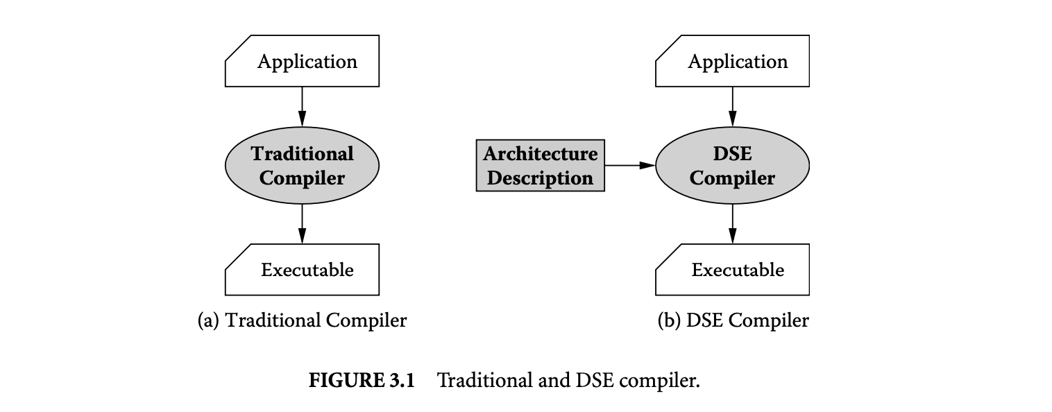
Given the significance of the compiler on processor power and performance, it is only logical that the compiler must play an important role in embedded processor design. To be able to use compilers to design processors, the key capability required is an architecture-sensitive compiler, or what we call a DSE compiler. It should be noted here that the DSE compiler we use and need here is conceptually different than a normal compiler. As depicted in Figure 3.1, a normal compiler is for a specific processor; it takes the source code of the application and generates code that is as fast as possible, as low-power consuming as possible, and so on for that specific processor. A DSE compiler is more generic; it is for a range of architectures. A DSE compiler takes the source code of the application, and the processor architecture description as input, and generates code for the processor described. The main difference between a normal compiler and a DSE compiler is in the heuristics used. The heuristics deployed in a traditional compiler may not have a large degree of parameterization. For example, the register allocator in the compiler for a machine that has 32 registers needs to be efficient in allocating just 32 registers, while a DSE compiler should be able to efficiently register allocate using any number of registers. One example is that the instruction scheduling heuristic of a DSE compiler will be parameterized on the processor pipeline description, while in a normal compiler, it can be fixed. Another example is the register allocation heuristic in the compiler. The register allocation algorithm in a compiler for a machine that has 32 registers needs to be efficient in allocating just 32 registers, while a DSE compiler should be able to efficiently register allocate using any number of registers. No doubt, all compilers have some degree of parameterizations that allow some degree of compiler code reuse when developing a compiler for a different architecture. DSE compilers have an extremely high degree of parametrization and allow large-scale compiler code reuse.
Additionally, while a normal compiler can have ad hoc heuristics to generate code, a DSE compiler needs to truthfully and accurately model the architecture and have compilation heuristics that are parameterized on the architecture model. For example, simple scheduling rules are often used to generate code for a particular bypass configuration. The scheduling rules, for example, a dependent load instruction should always be separated by two or more cycles after the add instruction, work for the specific bypass configuration. A DSE compiler will have to model the processor pipeline and bypasses as a graph or a grammar and generate code that selects instructions that form a path in the pipeline or a legitimate word in the grammar.
The DSE compiler gets the processor description in Architecture Description Language (ADL). While there is a significant body of research in developing ADLs[1, 4, 5, 8, 9, 20, 21, 38] to serve as golden specification for simulation, verification, synthesis, and so on, here we need an ADL that can describe the processor at an abstraction that the compiler needs. We use the EXPRESSION ADL [10, 25] to parameterize our DSE compiler that we call EXPRESS [13].
3.2.4.2 Traditional Design Space Exploration
Figure 3.2 models the traditional design methodology for exploring processor architectures. In the traditional approach, the application is compiled once to generate an executable. The executable is then
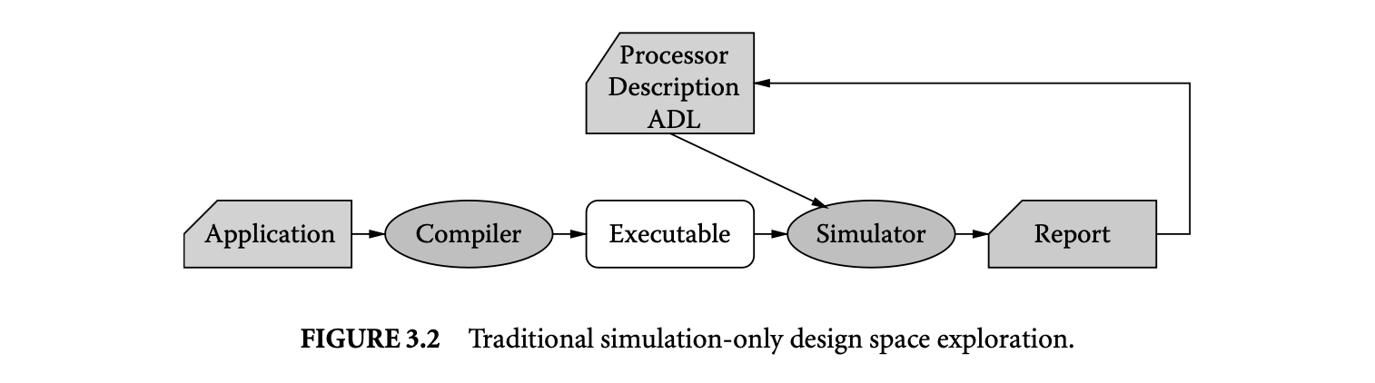
simulated over various architectures to choose the best architecture. We call such traditional design methodology simulation-only (SO) DSE. The SO DSE of embedded systems does not incorporate compiler effects in the embedded processor design. However, the compiler effects on the eventual power and performance characteristics can be incorporated in embedded processor design in an ad hoc manner in the existing methodology. For example, the hand-generated code can be used to reflect the code the actual compiler will eventually generate. This hand-generated code can be used to evaluate the architecture. However, such a scheme may be erroneous and result in suboptimal design decisions. A systematic way to incorporate compiler hints while designing the embedded processor is needed.
3.2.4.3 Compiler-in-the-Loop Exploration
Figure 3.3 describes our proposed CIL schema for DSE. In this scheme, for each architectural variation, the application is compiled (using the DSE compiler), and the executable is simulated on a simulator of the architectural variation. Thus, the evaluation of the architecture incorporates the compiler effects in a systematic manner. The overhead CIL DSE is the extra compilation time during each exploration step, but that is insignificant relative to the simulation time.
We have developed various novel compilation techniques to exploit architectural features present in embedded processors and demonstrate the need and usefulness of CIL DSE at several abstractions of processor design, as shown in Figure 3.4: at the processor instruction set design abstraction, at the processor pipeline design abstraction, at the memory design abstraction, and at the processor memory interaction abstraction.
At the processor pipeline design abstraction, we developed a novel compilation technique for generating code for processors with partial bypassing. Partial bypassing is a popular microarchitectural feature present in embedded systems because although full bypassing is the best for performance, it may have significant area, power, and wiring complexity overheads. However, partial bypassing in processors poses a challenge for compilers, as no techniques accurately detect pipeline hazards in partially bypassed processors. Our operation-table-based modeling of the processor allows us to accurately detect all kinds of pipeline hazards and generates up to 20% better performing code than a bypass-insensitive compiler [23, 32, 34].
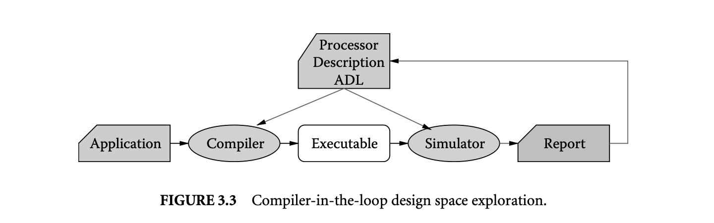

During processor design, the decision to add or remove a bypass is typically made by designer's intuition or SO DSE. However, since the compiler has significant impact on the code generated for a bypass configuration, the SO DSE may be significantly inaccurate. The comparison of our CIL with SO DSE demonstrates that not only do these two explorations result in significantly different evaluations of each bypass configuration, but they also exhibit different trends for the goodness of bypass configurations. Consequently, the traditional SO DSE can result in suboptimal design decisions, justifying the need and usefulness of our CIL DSE of bypasses in embedded systems [26, 31].
At the instruction set design abstraction, we first develop a novel compilation technique to generate code to exploit reduced bit-width instruction set architectures (rISAs). rISA is a popular architectural feature in which the processor supports two instruction sets. The first instruction set is composed of instructions that are 32 bits wide, and the second is a narrow instruction set composed of 16-bit-wide instructions. rISAs were originally conceived to reduce the code size of the application. If the application can be expressed in the narrow instructions only, then up to 50% code compression can be achieved. However, since the narrow instructions are only 16 bits wide, they implement limited functionality and can access only a small subset of the architectural registers. Our register pressure heuristic consistently achieves 35% code compression as compared to 14% achieved by existing techniques [12, 30].
In addition, we find out that the code compression achieved is very sensitive on the narrow instruction set chosen and the compiler. Therefore, during processor design, the narrow instruction set should be designed very carefully. We employ our CIL DSE technique to design the narrow instruction set. We find that correctly designing the narrow instruction set can double the achievable code compression [9, 29].
At the processor pipeline-memory interface design abstraction, we first develop a compilation technique to aggregate the processor activity and therefore reduce the power consumption when the processor is stalled. Fast and high-bandwidth memory buses, although best for performance, can have very high costs, energy consumption, and design complexity. As a result, embedded processors often employ slow buses. Reducing the speed of the memory bus increases the time a processor is stalled. Since the energy consumption of the processor is lower in the stalled state, the power consumption of the processor decreases. However, there is further scope for power reduction of the processor by switching the processor to IDLE state while it is stalled. However, switching the state of the processor takes 180 processor cycles in the Intel XScale, while the largest stall duration observed in the qsort benchmark of the MiBench suite is less than 100 processor cycles. Therefore, it is not possible to switch the processor to a low-power IDLE state during naturally occurring stalls during the application execution. Our technique aggregates the memory stalls of a processor into a large enough stall so that the processor can be switched to the low-power IDLE state. Our technique is able to aggregate up to 50,000 stall cycles, and by switching the processor to the low-power IDLE state, the power consumption of the processor can be reduced by up to 18% [33].
There is a significant difference in the processor power consumption between the SO DSE and CIL DSE. SO DSE can significantly overestimate the processor power consumption for a given memory bus configuration. This bolsters the need and usefulness of including compiler effects during the exploration and therefore highlights the need for CIL DSE.
This chapter uses a very simple architectural feature called horizontally partitioned caches (HPCs) to demonstrate the need and usefulness of CIL exploration design methodology. HPC is a popular memory architectural feature present in embedded systems in which the processors have multiple (typically two) caches at the same level of memory hierarchy. Wisely partitioning data between the caches can result in performance and energy improvements. However, existing techniques target performance improvements and achieve energy reduction only as a by-product. First we will develop energy-oriented data partitioning techniques to achieve high degrees of energy reduction, with a minimal hit on performance [35], and then we show that compared to SO DSE of HPC configurations, CIL DSE results in discovering HPC configurations that result in significantly less energy consumption.
3.3 Horizontally Partitioned Cache
Caches are one of the major contributors of not only system power and performance, but also of the embedded processor area and cost. In the Intel XScale [17], caches comprise approximately 90% of the transistor count and 60% of the area and consume approximately 15% of the processor power [3]. As a result, several hardware, software, and cooperative techniques have been proposed to improve the effectiveness of caches.
Horizontally partitioned caches are one such feature. HPCs were originally proposed in 1995 by Gonzalez et al. [6] for performance improvement. HPCs are a popular microarchitectural feature and have been deployed in several current processors such as the popular Intel StrongArm [16] and the Intel XScale [17]. However, compiler techniques to exploit them are still in their nascent stages.
A horizontally partitioned cache architecture maintains multiple caches at the same level of hierarchy, but each memory address is mapped to exactly one cache. For example, the Intel XScale contains two data caches, a 32KB main cache and a 2KB mini-cache. Each virtual page can be mapped to either of the data caches, depending on the attributes in the page table entry in the data memory management unit. Henceforth in this paper we will call the additional cache the mini-cache and the original cache the main cache.
The original idea behind such cache organization is the observation that array accesses in loops often have low temporal locality. Each value of an array is used for a while and then not used for a long time. Such array accesses sweep the cache and evict the existing data (like frequently accessed stack data) out of the cache. The problem is worse for high-associativity caches that typically employ first-in-first-out page replacement policy. Mapping such array accesses to the small mini-cache reduces the pollution in the main cache and prevents thrashing, leading to performance improvements. Thus, a horizontally partitioned cache is a simple, yet powerful, architectural feature to improve performance. Consequently, most existing approaches for partitioning data between the horizontally partitioned caches aim at improving performance.
In addition to performance improvement, horizontally partitioned caches also result in a reduction in the energy consumption due to two effects. First, reduction in the total number of misses results in reduced energy consumption. Second, since the size of the mini-cache is typically small, the energy consumed per access in the mini-cache is less than that in the large main cache. Therefore, diverting some memory accesses to the mini-cache leads to a decrease in the total energy consumption. Note that the first effect is in line with the performance goal and was therefore targeted by traditional performance improvement optimizations. However, the second effect is orthogonal to performance improvement. Therefore, energy reduction by the second effect was not considered by traditional performance-oriented techniques. As we show in this paper, the second effect (of a smaller mini-cache) can lead to energy improvements even in the presence of slight performance degradation. Note that this is where the goals of performance improvement and energy improvement diverge.
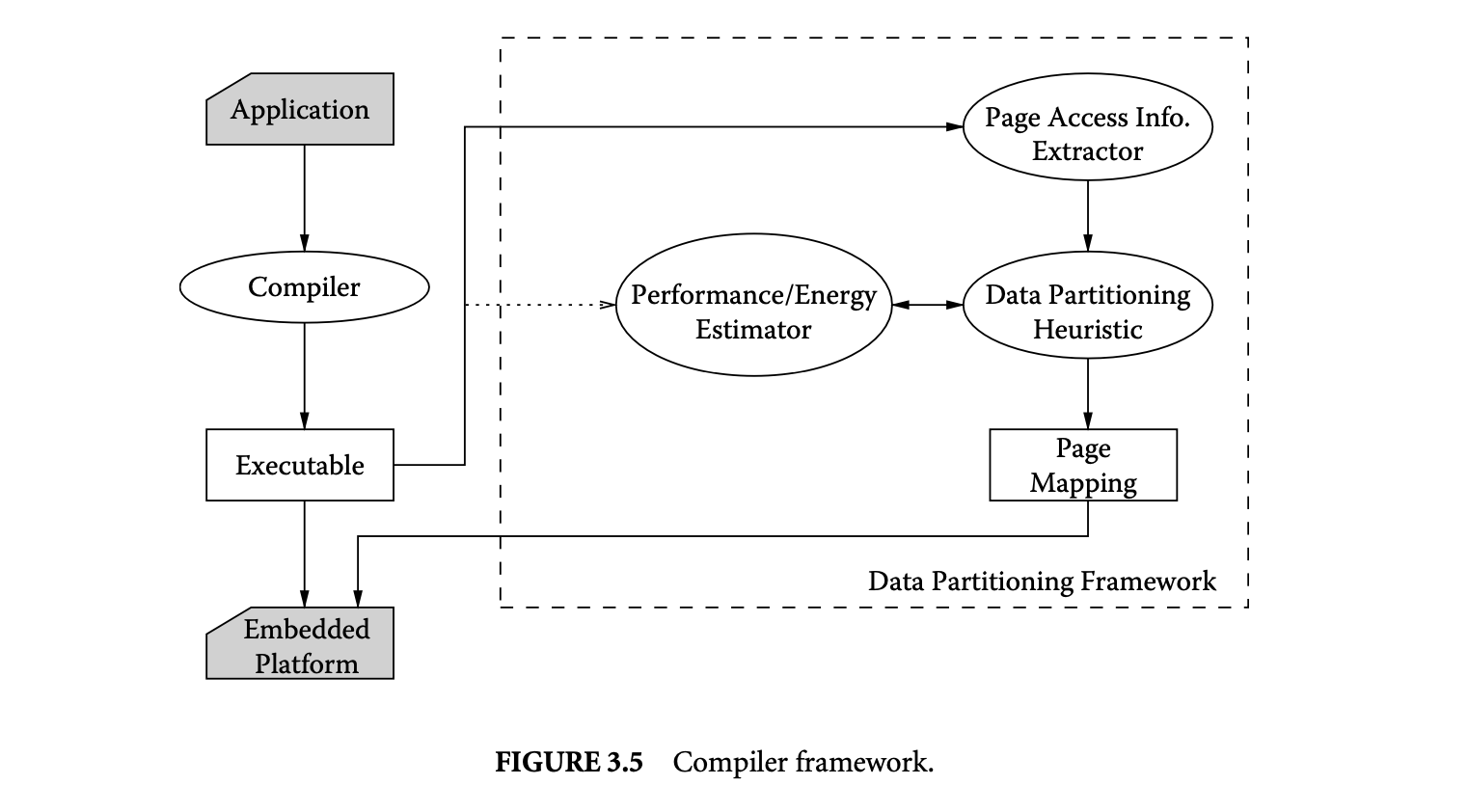
3.4 Compiler for Horizontally Partitioned Cache
3.4.1 HPC Compiler Framework
The problem of energy optimization for HPCs can be translated into a data partitioning problem. The data memory that the program accesses is divided into pages, and each page can be independently and exclusively mapped to exactly one of the caches. The compiler's job is then to find the mapping of the data memory pages to the caches that leads to minimum energy consumption.
As shown in Figure 3.5, we first compile the application and generate the executable. The page access information extractor calculates the number of times each page is accessed during the execution of the program. Then it sorts the pages in decreasing order of accesses to the pages. The complexity of simulation used to compute the number of accesses to each page and sorting the pages is , where is the number of data memory accesses, and is the number of pages accessed by the application.
The data partitioning heuristic finds the best mapping of pages to the caches that minimizes the energy consumption of the target embedded platform. The data partitioning heuristic can be tuned to obtain the best-performing, or minimal energy, data partition by changing the cost function performance/energy estimator.
The executable together with the page mapping are then loaded by the operating system of the target platform for optimized execution of the application.
3.4.2 Experimental Framework
We have developed a framework to evaluate data partitioning algorithms to optimize the memory latency or the memory subsystem energy consumption of applications. We have modified sim-safe simulator from the SimpleScalar toolset [2] to obtain the number of accesses to each data memory page. This implements our page access information extractor in Figure 3.5. To estimate the performance/energy of an application for a given mapping of data memory pages to the main cache and the mini-cache, we have developed performance and energy models of the memory subsystem of a popular PDA, the HP iPAQ h4300 [14].
Figure 3.6 shows the memory subsystem of the iPAQ that we have modeled. The iPAQ uses the Intel PXA255 processor [15] with the XScale core [17], which has a 32KB main cache and 2KB mini-cache. PXA255 also has an on-chip memory controller that communicates with via an off-chip bus. We have modeled the low-power 32MB Micron MT48V8M32LF [24] SDRAM as the off-chip memory. Since the iPAQ has 64MB of memory, we have modeled two SDRAMs.

We use the memory latency as the performance metric. We estimate the memory latency as , where and are the number of accesses, and and are the number of misses in the mini-cache and the main cache, respectively. We obtain these numbers using the sim-cache simulator [2], modified to model HPCs. The miss penalty was estimated as 25 processor cycles, taking into account the processor frequency (400 MHz), the memory bus frequency (100 MHz), the SDRAM access latency in power-down mode (6 memory cycles), and the memory controller delay (1 processor cycle).
We use the memory subsystem energy consumption as the energy metric. Our estimate of memory energy consumption has three components: energy consumed by the caches, energy consumed by off-chip busses, and energy consumed by the main memory (SDRAMs). We compute the energy consumed in the caches using the access and miss statistics from the modified sim-cache results. The energy consumed per access for each of the caches is computed using eCACTI [23]. Compared to CACTI [28], eCACTI provides better energy estimates for high-associativity caches, since it models sense-amps more accurately and scales device widths according to the capacitive loads. We have used linear extrapolation on cache size to estimate energy consumption of the mini-cache, since neither CACTI nor eCACTI model caches with less than eight sets.
We use the Printed Circuit Board (PCB) and layout recommendations of the PXA255 and Intel 440MX chipset [18, 16] and the relation between , and [19] to compute the the energy consumed by the external memory bus in a read/write burst as shown in Table 3.1.
We used the parameters shown in Table 3.2 from the MICRON MT48V8M32LF SDRAM to compute the energy consumed by the SDRAM per read/write burst operation (cache line read/write), shown in Table 3.2.
We perform our experiments on applications from the MiBench suite [7] and an implementation of the H.263 encoder [22]. To compile our benchmarks we used GCC with all optimizations turned on.
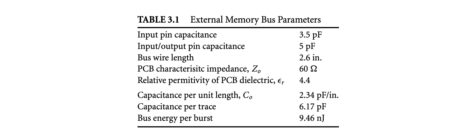

3.4.3 Simple Greedy Heuristics Work Well for Energy Optimization
In this section, we develop and explore several data partitioning heuristics with the aim of reducing the memory subsystem energy consumption.
3.4.3.1 Scope of Energy Reduction
To study the maximum scope of energy reduction achievable by page partitioning, we try all possible page partitions and estimate their energy consumption. Figure 3.7 plots the maximum energy reduction that we achieved by exhaustive exploration of all possible page mappings. We find the page partition that results in the minimum energy consumption by the memory subsystem and plot the reduction obtained compared to the case when all the pages are mapped to the main cache. Since the number of page partitions possible is exponential on the number of pages accessed by the application, it was not possible to complete the simulations for all the benchmarks. Exhaustive exploration was possible only for the first five benchmarks. The plot shows that compared to the case when all pages are mapped to the main cache, the scope of energy reduction is 55% on this set of benchmarks.
Encouraged by the effectiveness of page mapping, we developed several heuristics to partition the pages and see if it is possible to achieve high degrees of energy reduction using much faster techniques.
3.4.3.2 Complex Page Partitioning Heuristic: OM2N
The first technique we developed and examined is the heuristic OM2N, which is a greedy heuristic with one level of backtracking. Figure 3.8 describes the OM2N heuristic. Initially, (list of pages mapped to the main cache) and (list of pages mapped to the mini-cache) are empty. All the pages are initially undecided
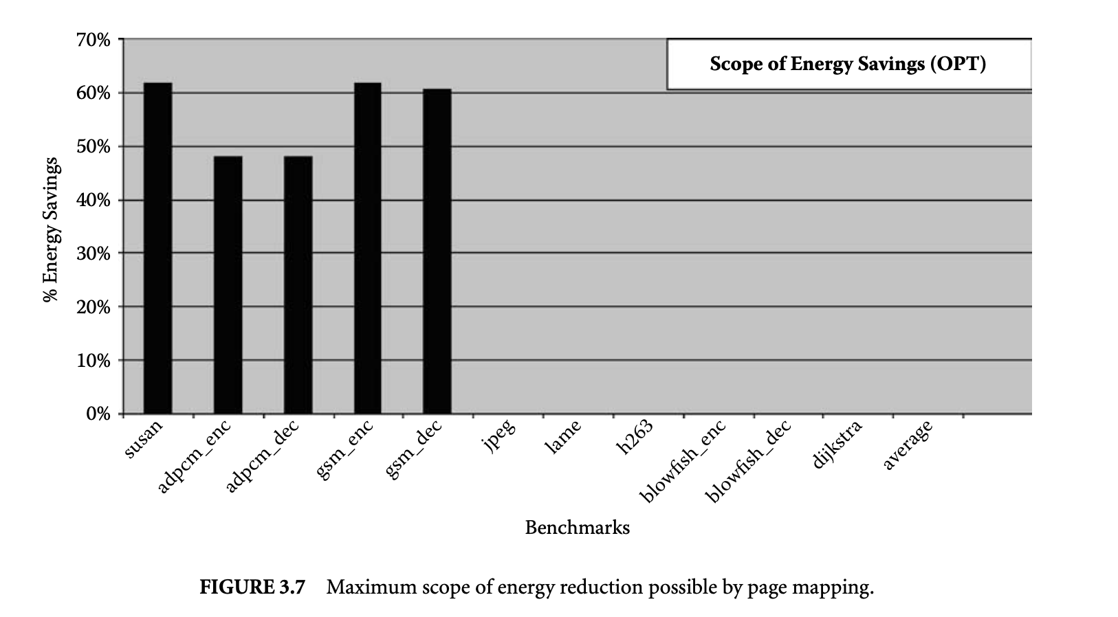
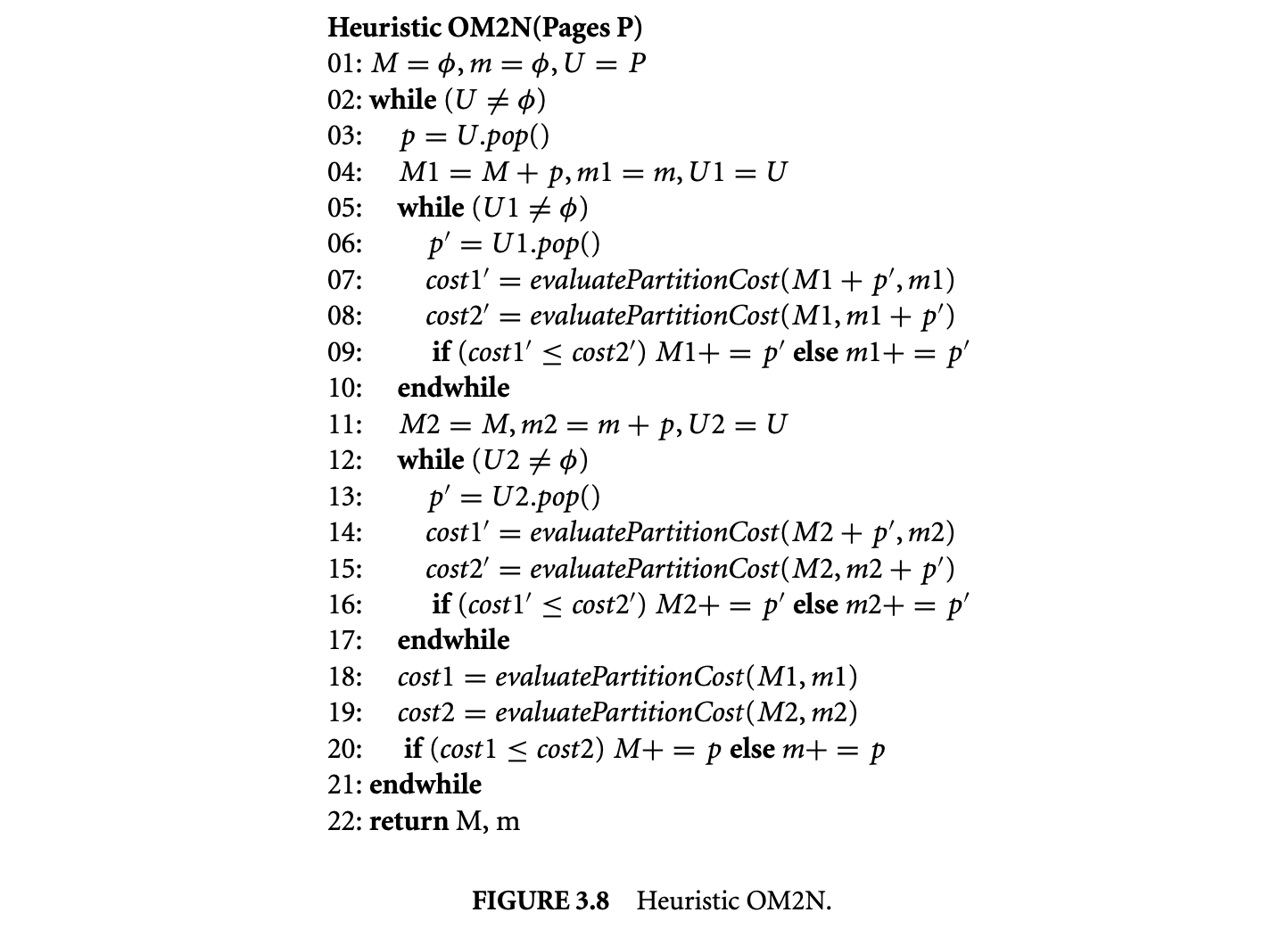
and are in (line 01). is a list containing pages sorted in decreasing order of accesses. The heuristic picks the first page in and tries both the mappings of this page -- first to the main cache (line 04) and then to the mini-cache (line 11). In lines 05 to 10, after mapping the first page to the main cache, the while loop tries to map each of the remaining pages one by one into the main cache (line 07) and the mini-cache (line 08) and keeps the best solution. Similarly, it tries to find the best page partition in lines 12 to 17 after assuming that the first page is mapped to the mini-cache and remembers the best solution. In lines 18 to 20 it evaluates the energy reduction achieved by the two assumptions. The algorithm finally decides on the mapping of the first page in line 20 by mapping the first page into the cache that leads to lesser energy consumption.
The function evaluatePartitionCost(M, m) uses simulation to estimate the performance or the energy consumption of a given partition. The simulation complexity, and therefore the complexity of the function evaluatePartitionCost(M, m), is O(). In each iteration of the topmost while loop in lines 02 to 21, the mapping of one page is decided. Thus, the topmost while loop in lines 02 to 21 is executed at most times. In each iteration of the while loop, the two while loops in lines 05 to 10 and lines 12 to 17 are executed. Each of these while loops may call the function evaluatePartitionCost(M, m) at most times. Thus, the time complexity of heuristic OM2N is O().
Figure 19 plots the energy reduction achieved by the minimum energy page partition found by our heuristic OM2N compared to the energy consumption when all the pages are mapped to the main cache. The main observation from Figure 19 is that the minimum energy achieved by the exhaustive and the OM2N is almost the same. On average, OM2N can achieve a 52% reduction in memory subsystem energy consumption.
3.4.3 Simple Page Partitioning Heuristic: OMN
Encouraged by the fact the algorithm of complexity O() can discover page mappings that result in near-optimal energy reductions, we tried to develop simpler and faster algorithms to partition the pages. Figure 20 is a greedy approach for solving the data partitioning problem. The heuristic picks the first page in and evaluates the cost of the partition when the page is mapped to the main cache (line 04) and when it is mapped to the mini-cache (line 05). The heuristic finally maps a page to the partition that results in minimum cost (line 06). There is only one while loop in this algorithm (lines 02 to 07), and in each step it decides upon the mapping of one page. Thus, it performs at most simulations, each of complexity . Thus, the complexity of this heuristic OMN is .

The leftmost bars in Figure 11 plot the energy reduction achieved by the minimum energy page partition found by our heuristic OMN compared to the energy consumption when all the pages are mapped to the main cache. On average, OMN can discover page mappings that result in a 50% reduction in memory subsystem energy consumption.
3.4.3.4 Very Simple Page Partitioning Heuristic: ON
Figure 12 shows a very simple single-step heuristic. If we define , then the first pages with the maximum number of accesses are mapped to the mini-cache, and the rest are mapped to the main cache. This partition aims to achieve energy reduction while making sure there is no performance loss (for high-associativity mini-caches). Note that for this heuristic we do not need to sort the list of all the pages. Only pages with the highest number of accesses are required. If the number of pages is , then the time complexity of selecting the pages with highest accesses is . Thus, the complexity of the heuristic is only , which can be approximated to , since both and are very small compared to .
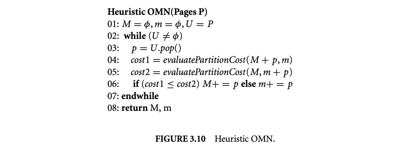
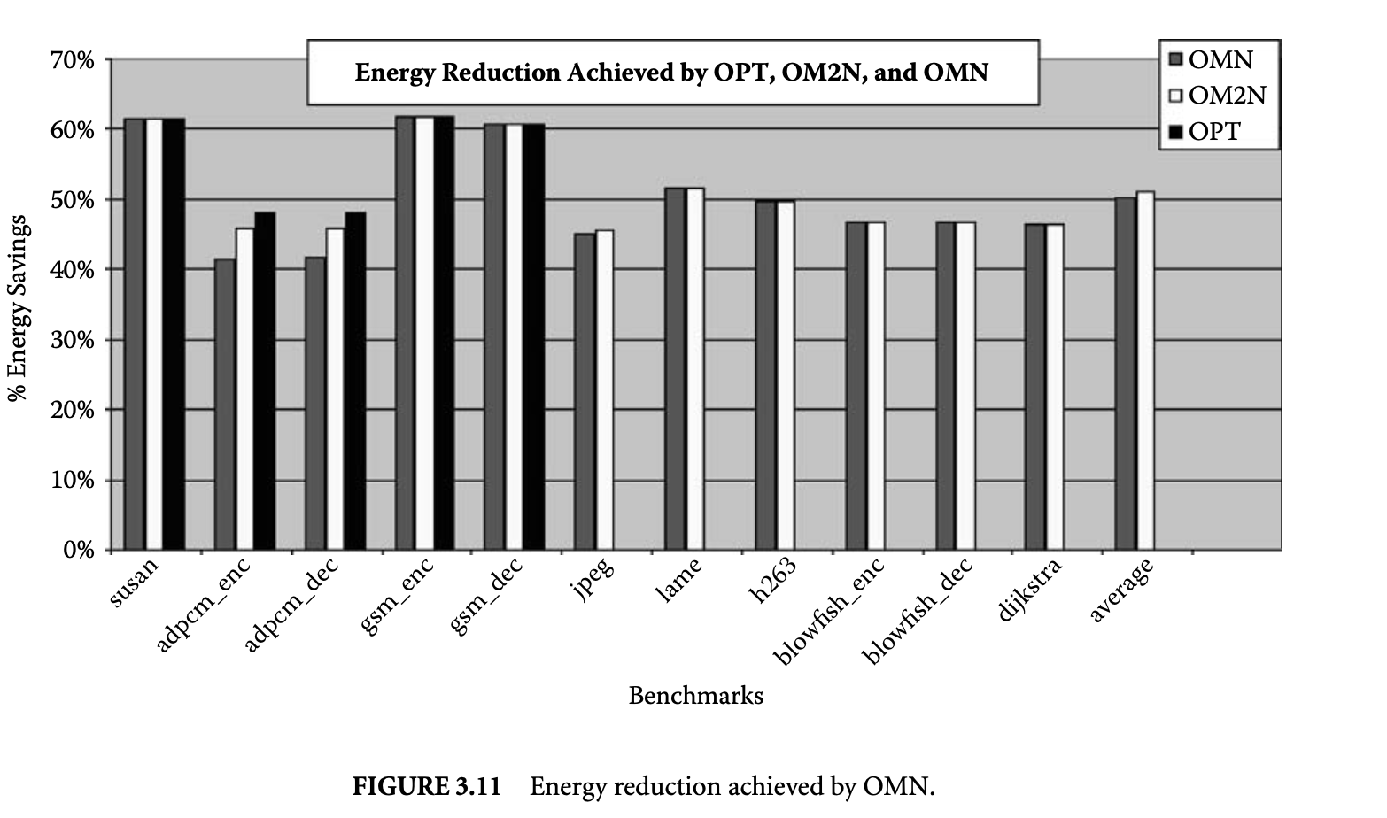
Figure 13 plots the energy reduction achieved by the minimum energy page partition found by our heuristic OMN compared to the energy consumption when all the pages are mapped to the main cache. On average, OMN can discover page mappings that result in a 5% reduction in memory subsystem energy consumption.
The leftmost bars in Figure 13 plot the energy reduction obtained by the lowest-energy-consuming page partition discovered by the ON heuristic compared to when all the pages are mapped to the main cache. Figure 13 shows that ON could not obtain as impressive results as the previous more complex heuristics. On average, the ON heuristic achieves only a 35% energy reduction in memory subsystem energy consumption.
3.4.3.5 Goodness of Page Partitioning Heuristics
We define the goodness of a heuristic as the energy reduction achieved by it compared to the maximum energy reduction that is possible, that is, , where is the energy consumption when all the pages are mapped to the main cache, is the energy consumption of the best energy partition the heuristic found, and is the energy consumption of the best energy partition. Figure 14 plots the goodness of the ON and OMN heuristic in obtaining energy reduction. For the last seven benchmarks for which we could not perform the optimal search. We assume the partition found by the heuristic OM2N is the best energy partition. The graph shows that the OMN heuristic could obtain on average 97% of the possible energy reduction, while ON could achieve on average 64% of the possible energy reduction. It is important to note that the GCC compiler for XScale does not exploit the mini-cache at all. The ON heuristic provides a simple yet effective way to exploit the mini-cache without incurring any performance penalty (for a high-associativity mini-cache).

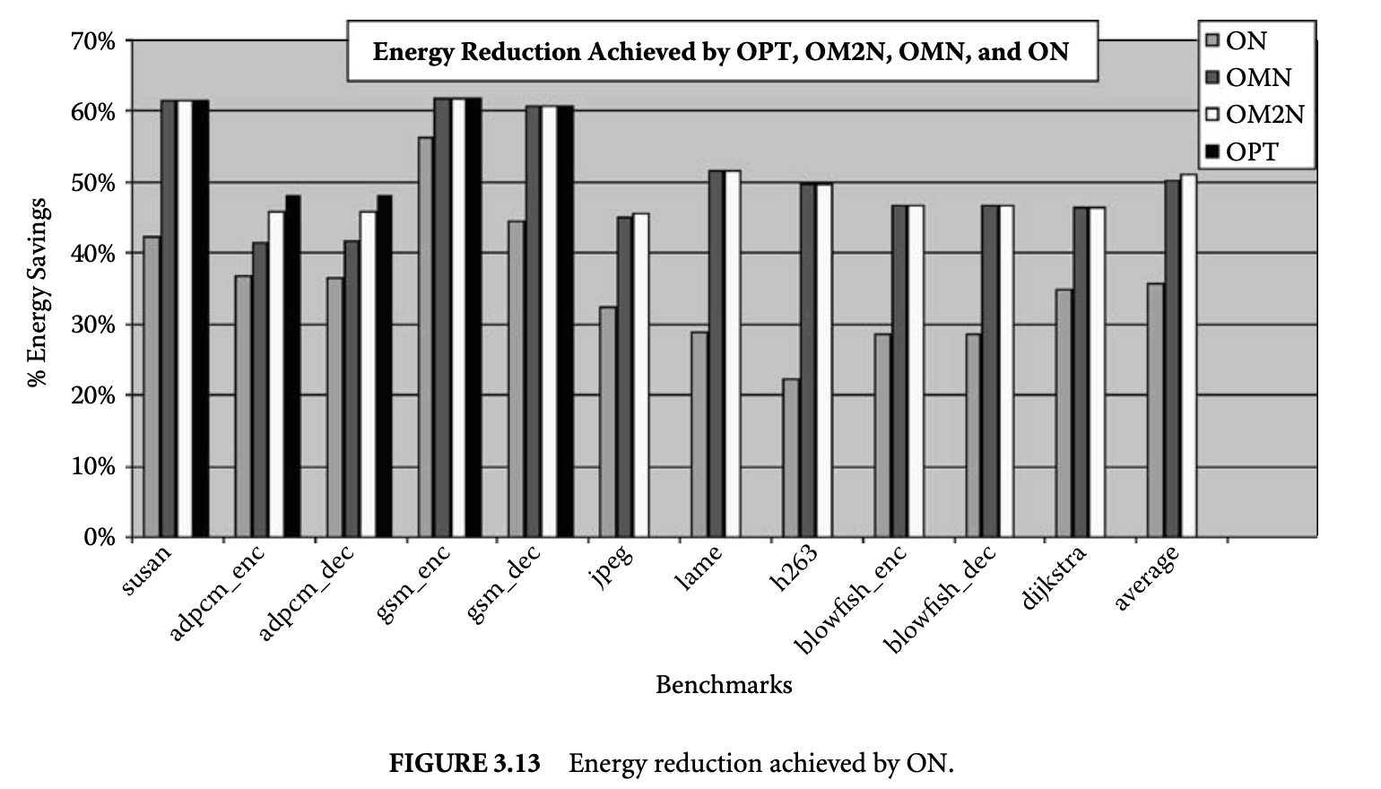
3.4.4 Optimizing for Energy Is Different Than Optimizing for Performance
This experiment investigates the difference in optimizing for energy and optimizing for performance. We find the partition that results in the least memory latency and the partition that results in the least energy consumption. Figure 3.15a plots , where is the memory subsystem energy consumption of the partition that results in the least memory latency, and is the memory subsystem energy consumption by the partition that results in the least memory subsystem energy consumption. For the first five benchmarks (susan to gsm_dec), the number of pages in the footprint were small, so we could explore all the partitions. For the last seven benchmarks (jpeg to dijkstra), we took the partition found by the OM2N heuristic as the best partition, as OM2N gives close-to-optimal results in cases when we were able to search optimally. The graph essentially plots the increase in energy if you choose the best performance partition as your design point. The increase in energy consumption is up to 130% and on average is 58% for this set of benchmarks.
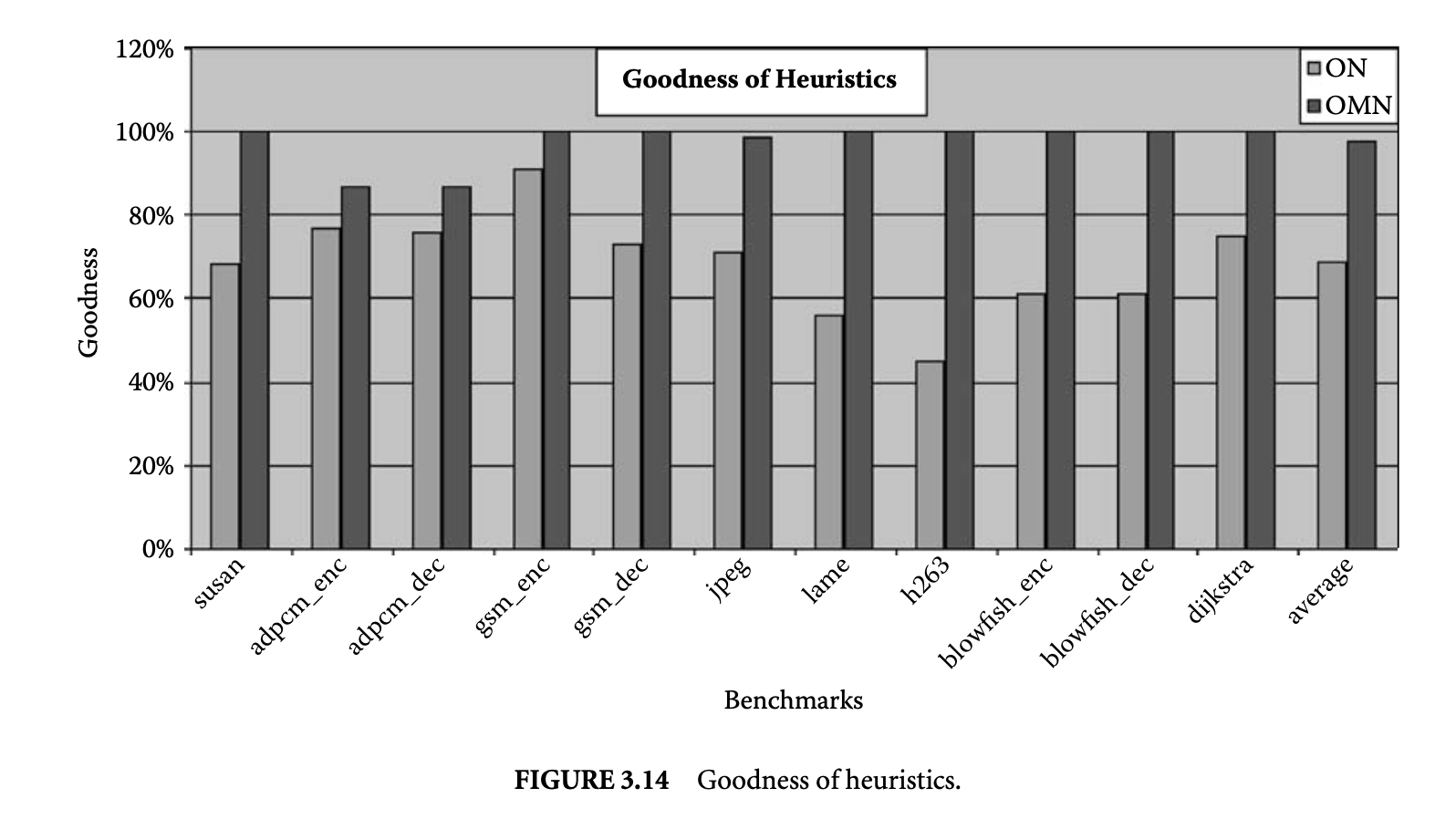
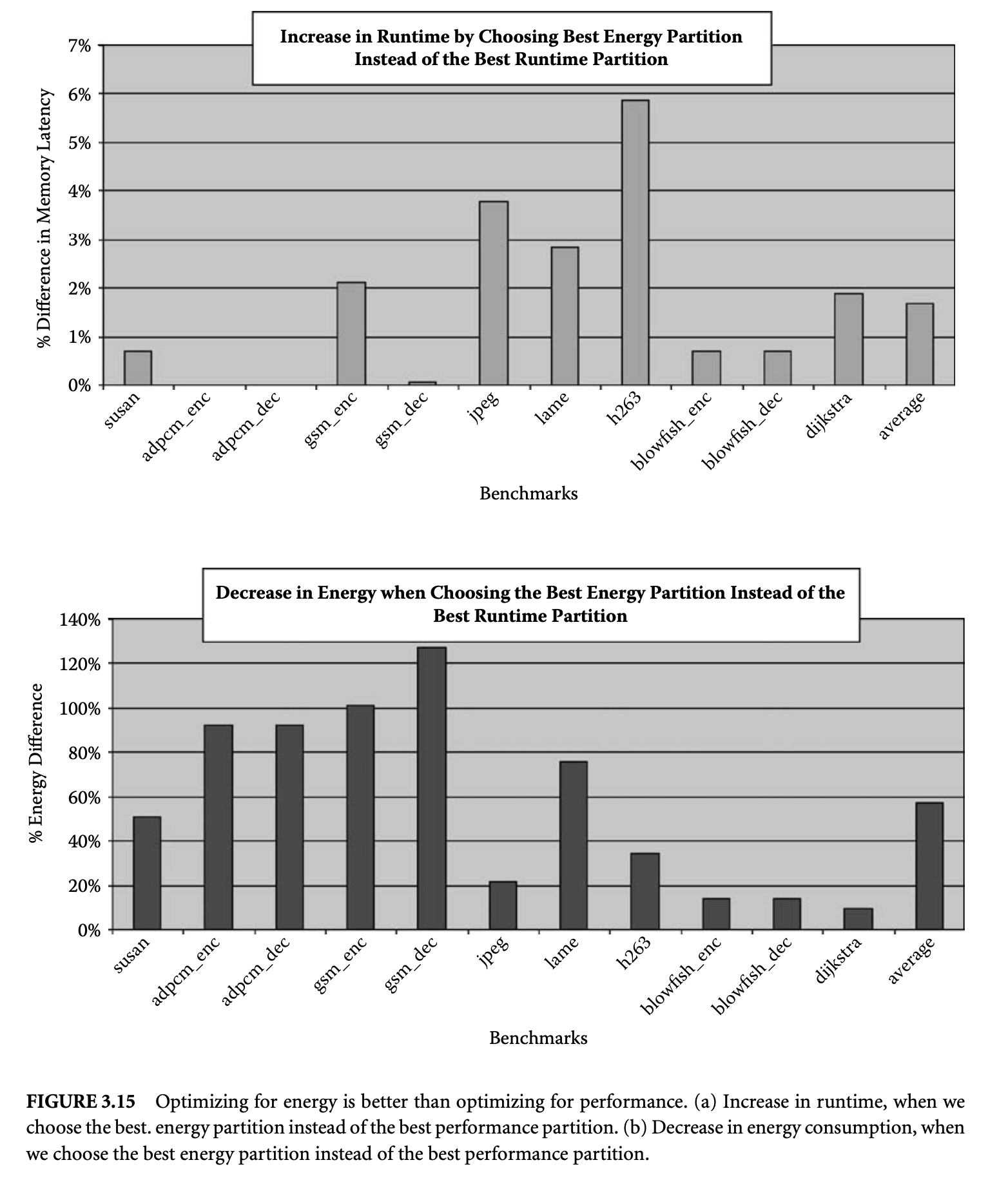
Figure 3.15: Optimizing for energy is better than optimizing for performance. (a) Increase in runtime, when we choose the best. energy partition instead of the best performance partition. (b) Decrease in energy consumption, when we choose the best energy partition instead of the best performance partition.
Figure 3.15b plots , where is the memory latency (in cycles) of the best energy partition, and is the memory latency of the best-performing partition. This graph shows the increase in memory latency when you choose the best energy partition compared to using the best performance partition. The increase in memory latency is on average 1.7% and is 5.8% in the worst case for this set of benchmarks. Thus, choosing the best energy partition results in significant energy savings at a minimal loss in performance.
3.5 Compiler-in-the-Loop HPC Design
So far we have seen that HPC is a very effective microarchitectural technique to reduce the energy consumption of the processor. The energy savings achieved are very sensitive to the HPC configuration; that is, if we change the HPC configuration, the page partitioning should also change.
In the traditional DSE techniques, for example, SO DSE, the binary and the page mapping are kept the same, and the binary with the page mapping is executed on different HPC configurations. This strategy is not useful for HPC DSE, since it does not make sense to use the same page mapping after changing the HPC parameters. Clearly, the HPC parameters should be explored with the CIL during the exploration. To evaluate HPC parameters, the page mapping should be set to the given HPC configuration.
Our CIL DSE framework to explore HPC parameters is depicted in Figure 3.16. The CIL DSE framework is centered around a textual description of the processor. For our purposes, the processor description contains information about (a) HPC parameters, (b) the memory subsystem energy models, and (c) the processor and memory delay models.
We use the OMN page partitioning heuristic and generate a binary executable along with the page mapping. The page mapping specifies to which cache (main or mini) each data memory page is mapped. The compiler is tuned to generate page mappings that lead to the minimum memory subsystem energy consumption. The executable and the page mapping are both fed into a simulator that estimates the runtime and the energy consumption of the memory subsystem.
The Design Space Walker performs HPC design space exploration by updating the HPC design parameters in the processor description. The mini-cache, which is configured by Design Space Walker, is specified using two attributes: the mini-cache size and the mini-cache associativity. For our experiments, we vary cache size from 256 bytes to 32 KB, in exponents of 2. We explore the whole range of mini-cache associativities, that is, from direct mapped to fully associative. We do not model the mini-cache configurations
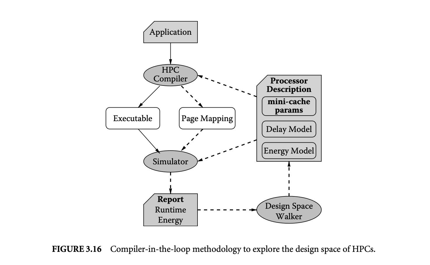
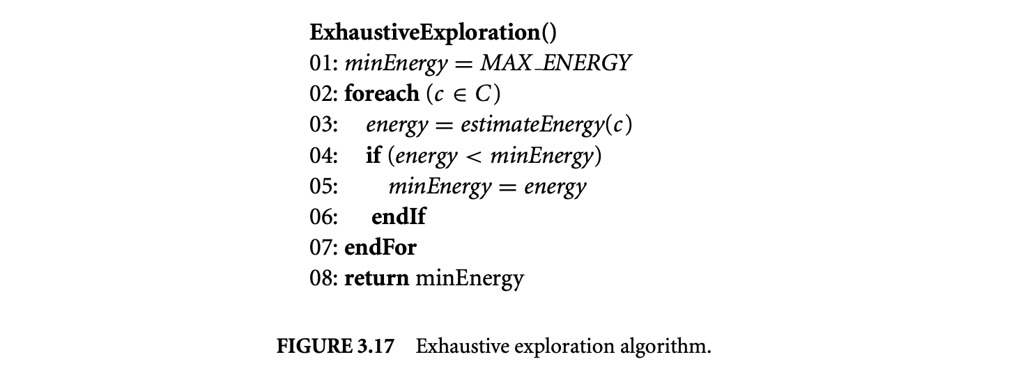
for which eCACTI [23] does not have a power model. We set the cache line size to be 32 bytes, as in the Intel XScale architecture. In total we explore 33 mini-cache configurations for each benchmark.
3.5.1 Exhaustive Exploration
We first present experiments to estimate the importance of exploration of HPCs. To this end, we perform exhaustive CIL exploration of HPC design space and find the minimum-energy HPC design parameters. Figure 3.17 describes the exhaustive exploration algorithm. The algorithm estimates the energy consumption for each mini-cache configuration (line 02) and keeps track of the minimum energy. The function estimate_energy estimates the energy consumption for a given mini-cache size and associativity.
Figure 3.18 compares the energy consumption of the memory subsystem with three cache designs. The leftmost bar represents the energy consumed by the memory subsystem when the system has only a 32KB
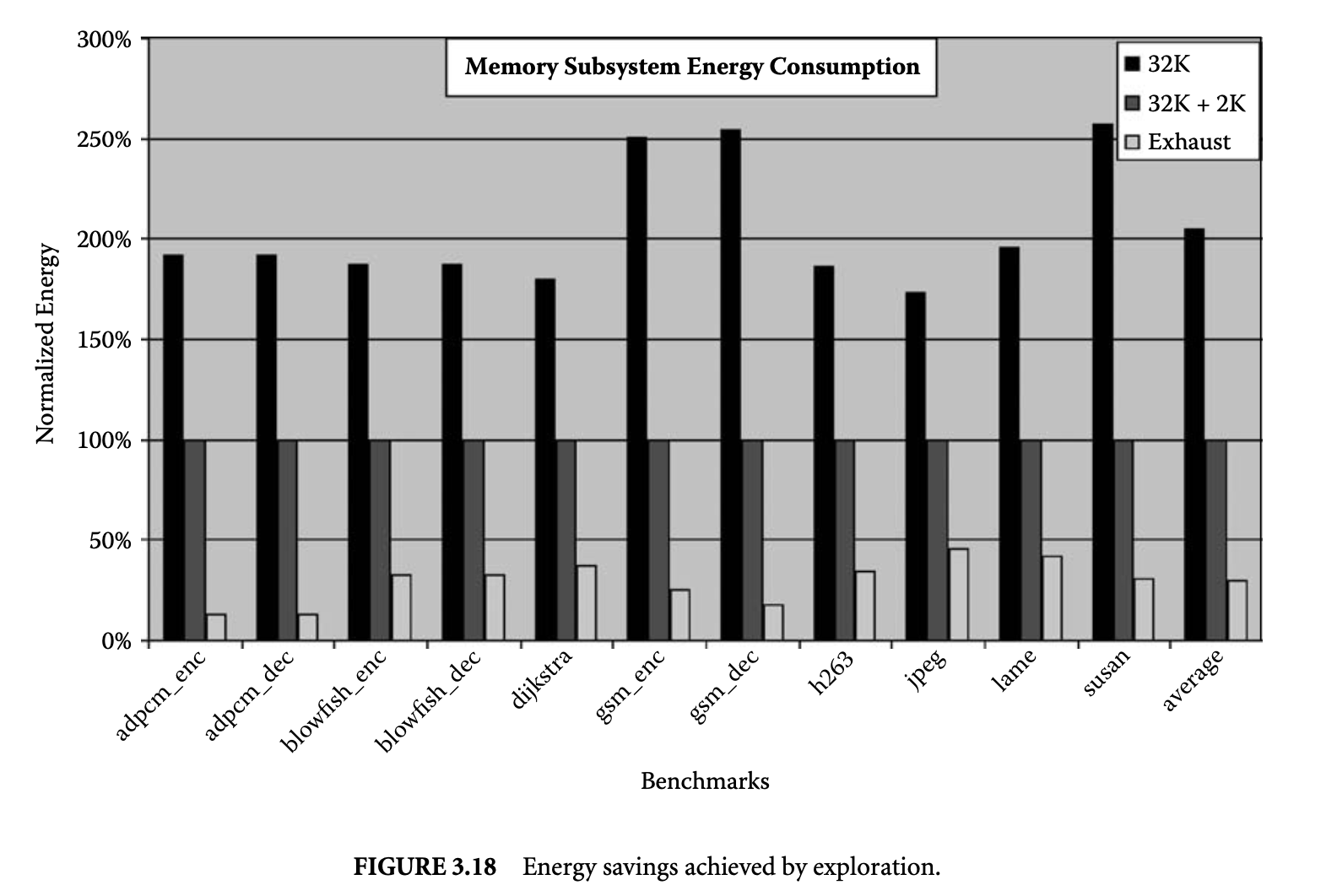
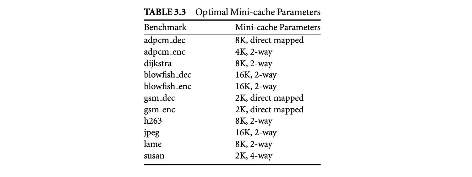
main cache (no mini-cache is present.) The middle bar shows the energy consumed when there is a 2KB mini-cache in parallel with the 32KB cache, and the application is compiled to achieve minimum energy. The rightmost bar represents the energy consumed by the memory subsystem, when the mini-cache parameters (size and associativity) are chosen using exhaustive CIL exploration. All the energy values are normalized to the case when there is a 2KB mini-cache (the Intel XScale configuration). The last set of bars is the average over the applications.
We make two important observations from this graph. The first is that HPC is very effective in reducing the memory subsystem energy consumption. Compared to not using any mini-cache, using a default mini-cache (the default mini-cache is 2KB, 32-way set associative) leads to an average of a 2 times reduction in the energy consumption of the memory subsystem. The second important observation is that the energy reduction obtained using HPCs is very sensitive to the mini-cache parameters. Exhaustive CIL exploration of the mini-cache DSE to find the minimum-energy mini-cache results in an additional 80% energy reduction, thus reducing the energy consumption to just 20% of the case with a 2KB mini-cache.
Furthermore, the performance of the energy-optimal HPC configuration is very close to the performance of the best-performing HPC configuration. The performance degradation was no more than 5% and was 2% on average. Therefore, energy-optimal HPC configuration achieves high energy reductions at minimal performance cost. Table 3.3 shows the energy-optimal mini-cache configuration for each benchmark. The table suggests that low-associativity mini-caches are good candidates to achieve low-energy solutions.
3.5.2 HPC CIL DSE Heuristics
We have demonstrated that CIL DSE of HPC design parameters is very useful and important to achieve significant energy savings. However, since the mini-cache design space is very large, exhaustive exploration may consume a lot of time. In this section we explore heuristics for effective and efficient HPC DSE.
3.5.2.1 Greedy Exploration
The first heuristic we develop for HPC CIL DSE is a pure greedy algorithm, outlined in Figure 3.19. The greedy algorithm first greedily finds the cache size (lines 02 to 04) and then greedily finds the associativity (lines 05 to 07). The function betterNewConfiguration tells whether the new mini-cache parameters result in lower energy consumption than the old mini-cache parameters.
Figure 3.20 plots the energy consumption when the mini-cache configuration is chosen by the greedy algorithm compared to when using the default 32KB main cache and 2KB mini-cache configuration. The plot shows that for most applications, greedy exploration is able to achieve good results, but for blowfish and susan, the greedy exploration is unable to achieve any energy reduction; in fact, the solution it has found consumes even more energy than the base configuration. However, on average, the greedy CIL HPC DSE can reduce the energy consumption of the memory subsystem by 50%.
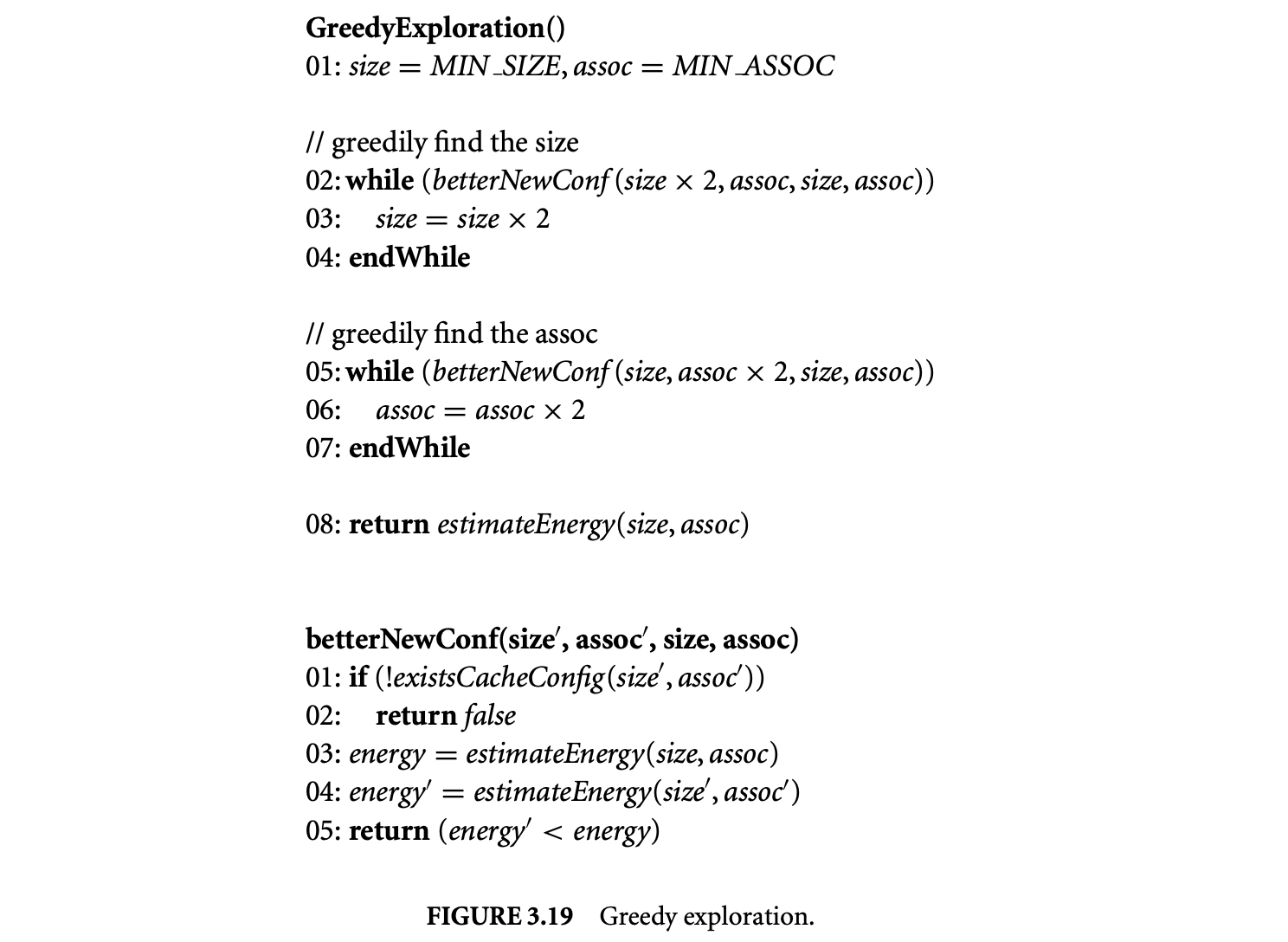
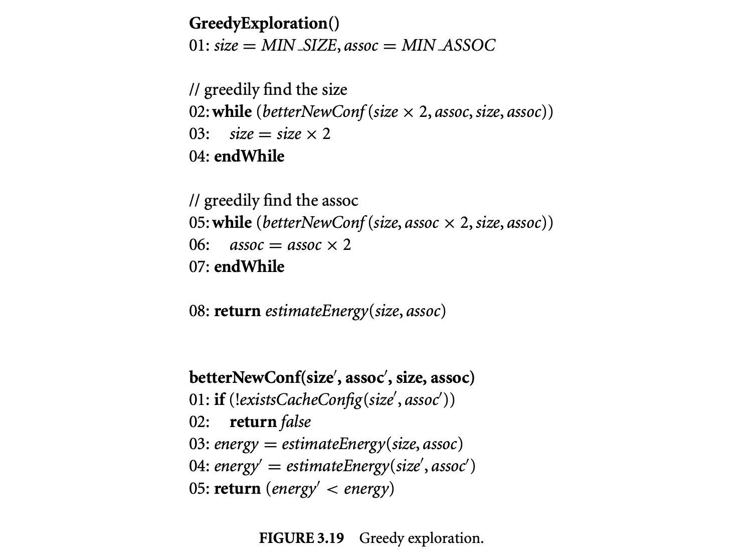
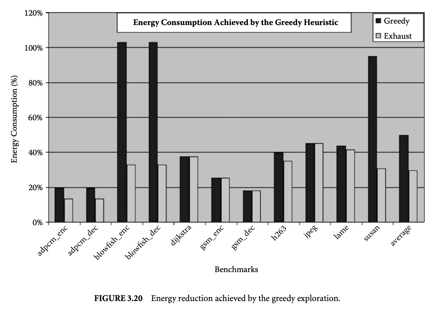
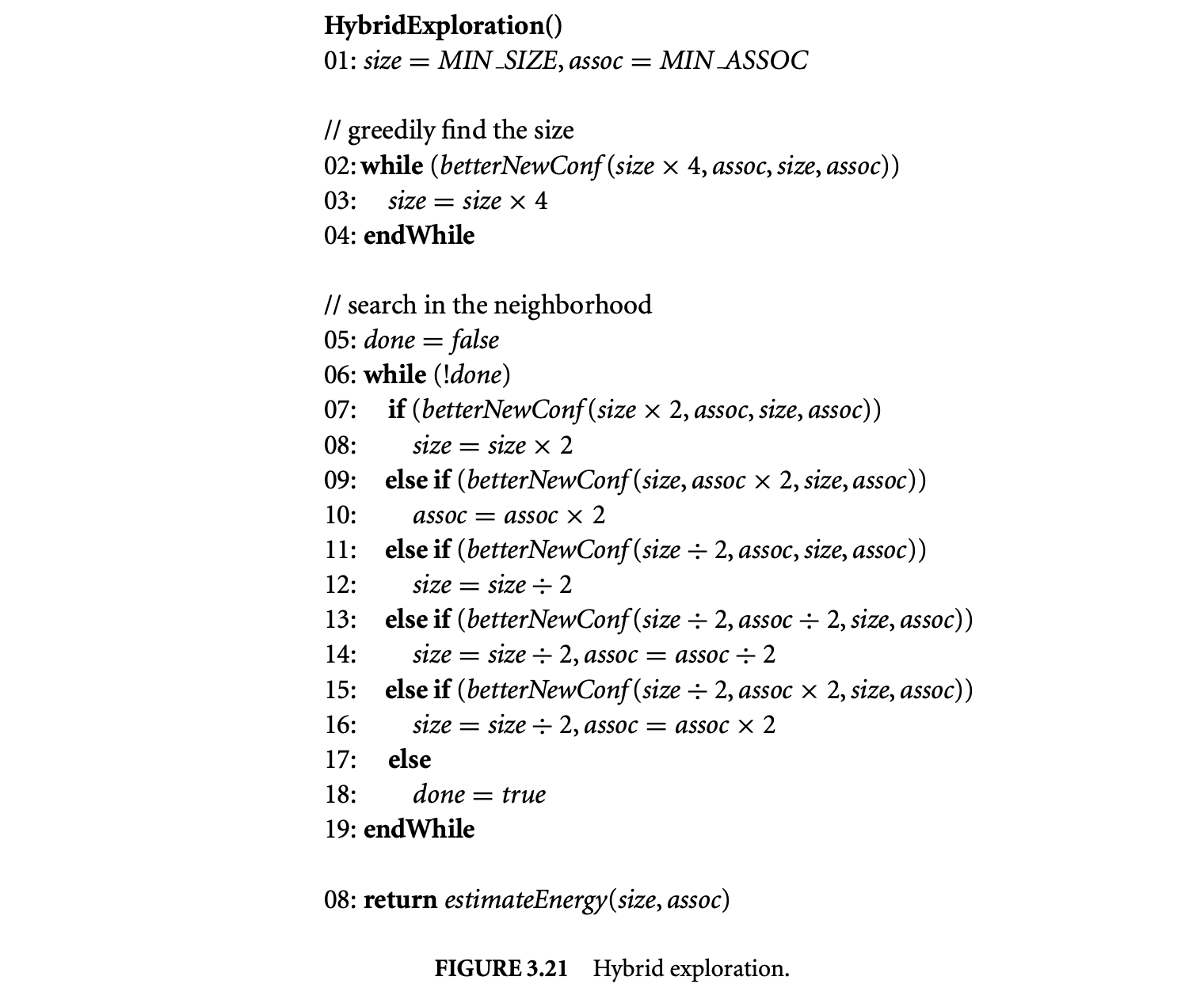
3.5.2.2 Hybrid Exploration
To achieve energy consumption close to the optimal configurations, we developed a hybrid algorithm, outlined in Figure 3.21. The hybrid algorithm first greedily searches for the optimal mini-cache size (lines 02 to 04). Note, however, that it tries every alternate mini-cache size. The hybrid algorithm tries mini-cache sizes in exponents of 4, rather than 2 (line 03). Once it has found the optimal mini-cache size, it explores exhaustively in the size-associativity neighborhood (lines 07 to 15) to find a better size-associativity configuration.
The middle bar in Figure 3.22 plots the energy consumption of the optimal configuration compared to the energy consumption when the XScale default 32-way, 2K mini-cache is used and compares the energy reductions achieved with the greedy and exhaustive explorations. The graph shows that the hybrid exploration can always find the optimal HPC configuration for our set of benchmarks.
3.5.2.3 Energy Reduction and Exploration Time Trade-Off
There is a clear trade-off between the energy reductions achieved by the exploration algorithms and the time required for the exploration. The rightmost bar in Figure 3.23 plots the time (in hours) required to explore the design space using the exhaustive algorithm. Although the exhaustive algorithm is able to discover extremely low energy solutions, it may take tens of hours to perform the exploration. The leftmost bar in Figure 3.23 plots the time that greedy exploration requires to explore the design space of the mini-cache. Although the greedy algorithm reduces the exploration time on average by a factor of 5 times, the energy consumption is on average 2 times more than what is achieved by the optimal algorithm.
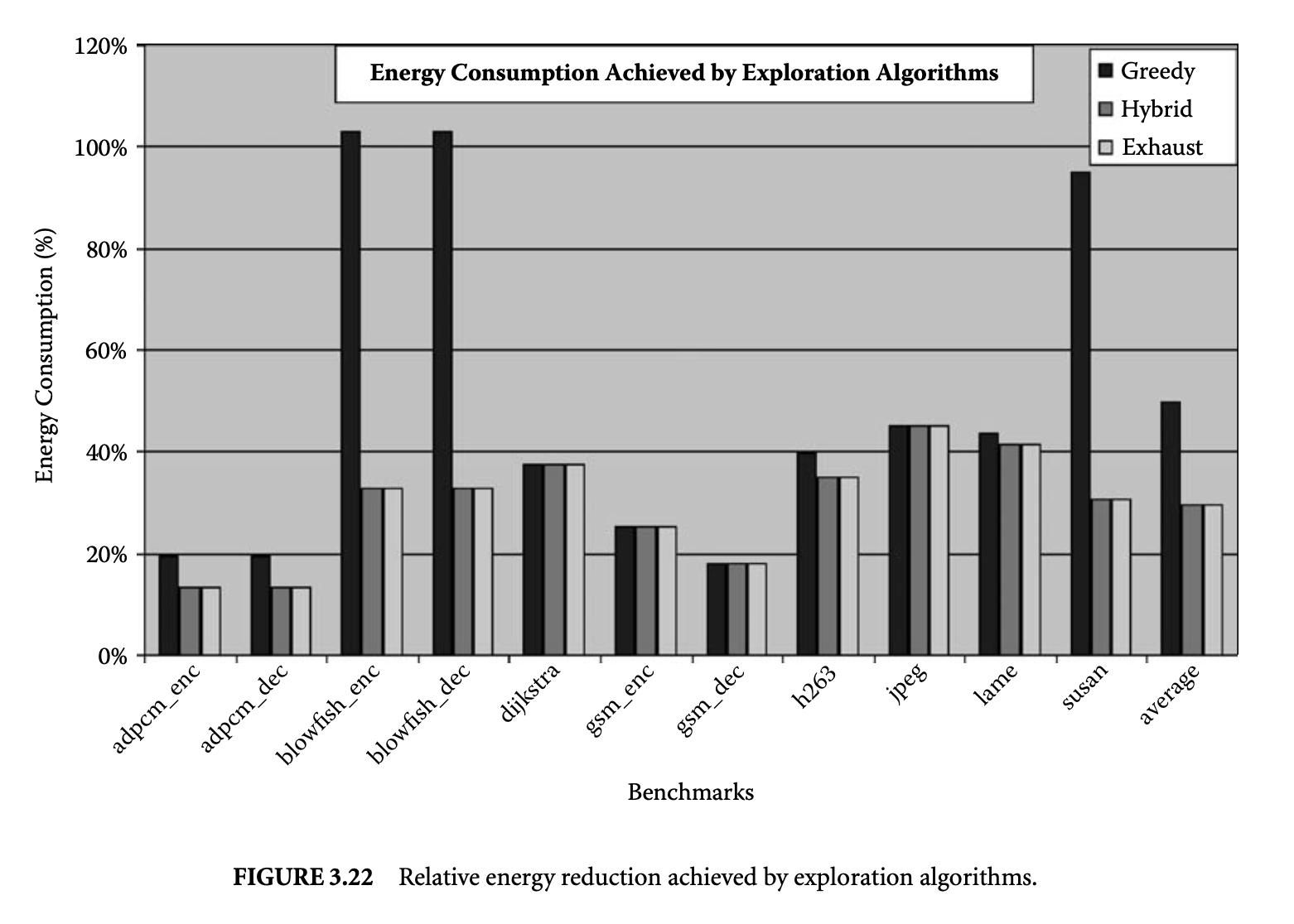
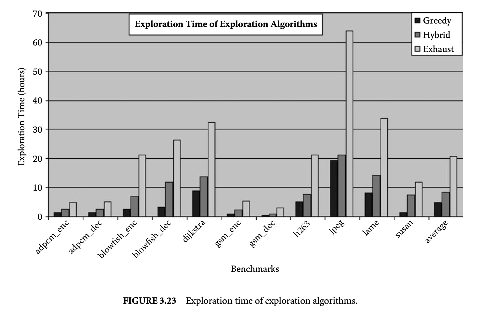
Finally, the middle bar in Figure 3.23 plots the time required to find the mini-cache configuration when using the hybrid algorithm. Our hybrid algorithm is able to find the optimal mini-cache configuration in all of our benchmarks, while it takes about 3 times less time than the optimal algorithm. Thus, we believe the hybrid exploration is a very effective and efficient exploration technique.
3.5.3 Importance of Compiler-in-the-Loop DSE
Our next set of experiments show that although SO DSE can also find HPC configurations with less memory subsystem energy consumption, it does not do as well as CIL DSE. To this end, we performed SO DSE of HPC design parameters. We compile once for the 32KB/2KB (i.e., the original XScale cache configuration) to obtain an executable and the minimum energy page mapping. While keeping these two the same, we explored all the HPC configurations to find the HPC design parameters that minimize the memory subsystem energy consumption. Figure 3.24 plots the the energy consumption of the HPC configuration found by the SO DSE (middle bar) and CIL DSE (right bar) and the original Intel XScale HPC configuration (left bar) for each benchmark. The rightmost set of bars represents the average over all the benchmarks. All the energy consumption values are normalized to energy consumption of the 32KB/2KB configuration.
It should be noted that the overhead of compilation time in CIL DSE is negligible, because simulation times are several orders of magnitude more than compilation times. The important observation to make from this graph is that although even SO DSE can find HPC configurations that result in, on average, a 57% memory subsystem energy reduction, CIL DSE is much more effective and can uncover HPC configurations that result in a 70% reduction in the memory subsystem energy reduction.
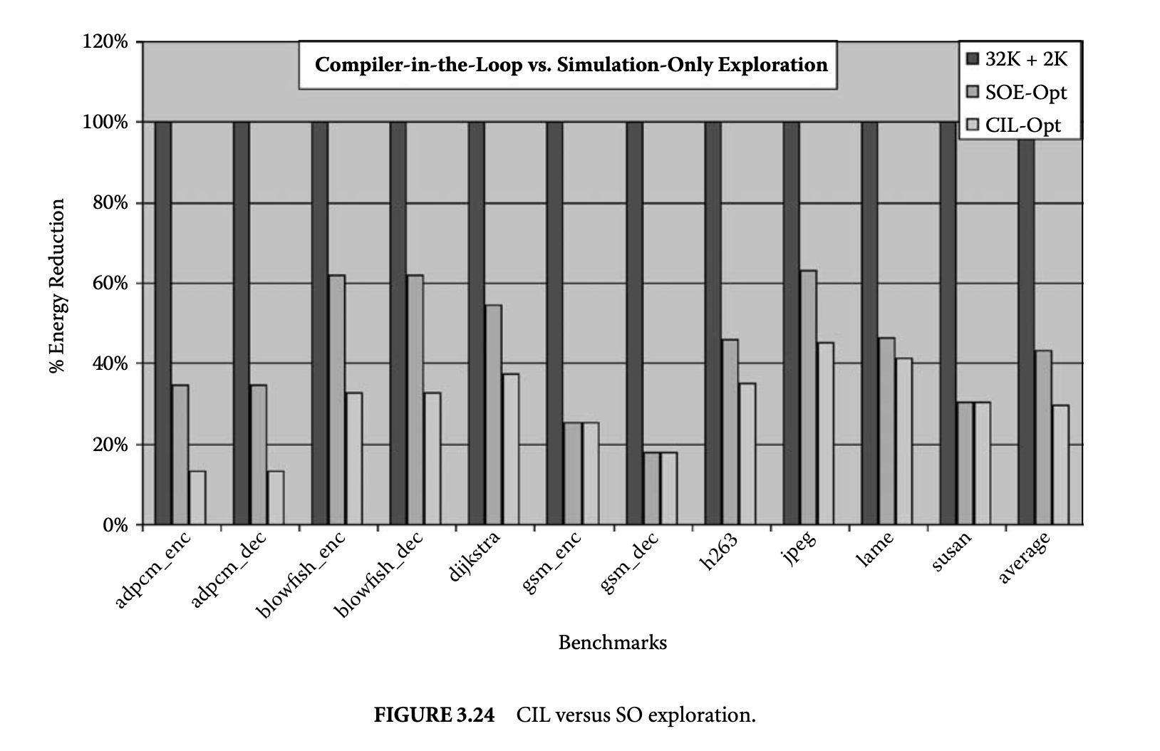
3.6 Summary
Embedded systems are characterized by stringent, application-specific, multidimensional constraints on their designs. These constraints, along with the shrinking time to market and frequent upgrade needs of embedded systems, are responsible for programmable embedded systems that are highly customized. While code generation for these highly customized embedded systems is a challenge, it is also very rewarding in the sense that an architecture-sensitive compilation technique can have significant impact on the system power, performance, and so on. Given the importance of the compiler on the system design parameters, it is reasonable for the compiler to take part in designing the embedded system. While it is possible to use ad hoc methods to include the compiler effects while designing an embedded system, a systematic methodology to design embedded processors is needed. This chapter introduced the CIL design methodology, which systematically includes the compiler in the embedded system DSE. Our methodology requires an architecture-sensitive compiler. To evaluate a design point in the embedded system design space, the application code is first compiled for the embedded system design and is then executed on the embedded system model to estimate the various design parameters (e.g., power, performance, etc.). Owing to the lack of compiler technology for embedded systems, most often, first an architecture-sensitive compilation technique needs to be developed, and only then can it be used for CIL design of the embedded processor. In the chapter we first developed a compilation technique for HPCs, which can result in a 50% reduction in the energy consumption of the memory subsystem. When we use this compilation technique in our CIL approach, we can come up with HPC parameters that result in an 80% reduction in the energy consumption by the memory subsystem, demonstrating the need and usefulness of our approach.
References
[1] M. R. Barbacci. 1981. Instruction set processor specifications (ISPS): The notation and its applications. IEEE Transactions on Computing C-30(1):24-40. New York: IEEE Press.
[2] D. Burger and T. M. Austin. 1997. The SimpleScalar tool set, version 2.0. SIGARCH Computer Architecture News 25(3):13-25.
[3] L. T. Clark, E. J. Hoffman, M. Biyani, Y. Liao, S. Strazdus, M. Morrow, K. E. Velarde, and M. A. Yarch. 2001. An embedded 32-b microprocessor core for low-power and high-performance applications. IEEE J. Solid State Circuits 36(11):1599-608. New York: IEEE Press.
[4] Paul C. Clements. 1996. A survey of architecture description languages. In Proceedings of International Workshop on Software Specification and Design (IWSSD), 16-25.
[5] A. Fauth, M. Freericks, and A. Knoll. 1993. Generation of hardware machine models from instruction set descriptions. In IEEE Workshop on VLSI Signal Processing, 242-50.
[6] A. Gonzalez, C. Aliagas, and M. Valero. 1995. A data cache with multiple caching strategies tuned to different types of locality. In ICS '95: Proceedings of the 9th International Conference on Supercomputing, 338-47. New York: ACM Press.
[7] M. R. Guthaus, J. S. Ringenberg, D. Ernst, T. M. Austin, T. Mudge, and R. B. Brown. 2001. MiBench: A free, commercially representative embedded benchmark suite. In IEEE Workshop in Workload Characterization.
[8] J. Gyllenhaal, B. Rau, and W. Hwu. 1996. HMDES version 2.0 specification. Tech. Rep. IMPACT-96-3, IMPACT Research Group, Univ. of Illinois, Urbana.
[9] G. Hadjiyiannis, S. Hanono, and S. Devadas. 1997. ISDL: An instruction set description language for retargetability. In Proceedings of Design Automation Conference (DAC), 299-302. New York: IEEE Press.
[10] A. Halambi, P. Grun, V. Ganesh, A. Khare, N. Dutt, and A. Nicolau. 1999. EXPRESSION: A language for architecture exploration through compiler/simulator retargetability. In Proceedings of Design Automation and Test in Europe. New York: IEEE Press.
[11] A. Halambi, A. Shrivastava, P. Biswas, N. Dutt, and A. Nicolau. 2002. A design space exploration framework for reduced bit-width instruction set architecture (risa) design. In ISS '02: Proceedings of the 15th International Symposium on System Synthesis, 120-25. New York: ACM Press.
[12] A. Halambi, A. Shrivastava, P. Biswas, N. Dutt, and A. Nicolau. 2002. An efficient compiler technique for code size reduction using reduced bit-width isas. In Proceedings of the Conference on Design, Automation and Test in Europe. New York: IEEE Press.
[13] A. Halambi, A. Shrivastava, N. Dutt, and A. Nicolau. 2001. A customizable compiler framework for embedded systems. In Proceedings of SCOPES.
[14] Hewlett Packard. HP iPAQ 14000 series-system specifications. http://www.hp.com.
[15] Intel Corporation. Intel PXA255 processor: Developer's manual. http://www.intel.com/design/pca/applicationsprocessors/manuals/278693.htm.
[16] Intel Corporation. Intel StrongARM SA-1110 microprocessor brief datasheet. http://download.intel.com/design/strong/datashts/27824105.pdf.
[17] Intel Corporation. Intel XScale(R) Core: Developer's manual. http://www.intel.com/design/intelxscale/273473.htm.
[18] Intel Corporation. LV/ULV Mobile Intel Pentium III Processor-M and LV/ULV Mobile Intel Celeron Processor (0.13u)/Intel 440MX Chipset: Platform design guide. http://www.intel.com/design/mobile/desguide/251012.htm.
[19]IPC-D-317A: Design guidelines for electronic packaging utilizing high-speed techniques. 1995. Institute for Interconnecting and Packaging Electronic Circuits.
[20] D. Kastner. 2000. TDL: A hardware and assembly description language. Tech. Rep. TDL 1.4, Saarland University, Germany.
[21] R. Leupers and P. Marwedel. 1998. Retargetable code generation based on structural processor descriptions. Design Automation Embedded Syst. 3(1):75-108. New York: IEEE Press.
[22] K. Lillevold et al. 1995. H.263 test model simulation software. Telenor R&D.
[23] M. Mamidipaka and N. Dutt. 2004. eCACTI: An enhanced power estimation model for on-chip caches. Tech. Rep. TR-04-28, CECS, UCI.
[24] Micron Technology, Inc. MICRON Mobile SDRAM MT48V8M32LF datasheet. http://www.micron.com/products/dram/mobilesdram/.
[25] P. Mishra, A. Shrivastava, and N. Dutt. 2004. Architecture description language (adl)-driven software toolkit generation for architectural exploration of programmable socs. In DAC '04: Proceedings of the 41st Annual Conference on Design Automation, 626-58. New York: ACM Press.
[26] S. Park, E. Earlie, A. Shrivastava, A. Nicolau, N. Dutt, and Y. Paek. 2006. Automatic generation of operation tables for fast exploration of bypasses in embedded processors. In DATE '06: Proceedings of the Conference on Design, Automation and Test in Europe, 1197-202. Leuven, Belgium: European Design and Automation Association. New York: IEEE Press.
[27] S. Park, A. Shrivastava, N. Dutt, A. Nicolau, Y. Paek, and E. Earlie. 2006. Bypass aware instruction scheduling for register file power reduction, In LCTES 2006: Proceedings of the 2006 ACM SIGPLAN/SIGBED conference on language, compilers, and tool support for embedded systems, 173-81. New York: ACM Press.
[28] P. Shivakumar and N. Jouppi. 2001. Cacti 3.0: An integrated cache timing, power, and area model. WRL Technical Report 2001/2.
[29] A. Shrivastava, P. Biswas, A. Halambi, N. Dutt, and A. Nicolau. 2006. Compilation framework for code size reduction using reduced bit-width isas (risas). ACM Transaction on Design Automation of Electronic Systems 11(1):123-46. New York: ACM Press.
[30] A. Shrivastava and N. Dutt. 2004. Energy efficient code generation exploiting reduced bit-width instruction set architecture. In Proceedings of The Asia Pacific Design Automation Conference (ASPDAC). New York: IEEE Press.
[31] A. Shrivastava, N. Dutt, A. Nicolau, and E. Earlie. 2005. Pbexplore: A framework for compiler-in-the-loop exploration of partial bypassing in embedded processors. In DATE '05: Proceedings of the Conference on Design, Automation and Test in Europe, 1264-69. Washington, DC: IEEE Computer Society.
[32] A. Shrivastava, E. Earlie, N. D. Dutt, and A. Nicolau. 2004. Operation tables for scheduling in the presence of incomplete bypassing. In CODES+ISSS, 194-99. New York: IEEE Press.
[33] A. Shrivastava, E. Earlie, N. Dutt, and A. Nicolau. 2005. Aggregating processor free time for energy reduction. In CODES+ISSS '05: Proceedings of the 3rd IEEE/ACM/IFIP International Conference on Hardware/Software Codesign and System Synthesis, 154-59. New York: ACM Press.
[34] A. Shrivastava, E. Earlie, N. Dutt, and A. Nicolau. 2006. Retargetable pipeline hazard detection for partially bypassed processors, In IEEE Transactions on Very Large Scale Integrated Circuits, 791-801. New York: IEEE Press.
[35] A. Shrivastava, I. Issenin, and N. Dutt. 2005. Compilation techniques for energy reduction in horizontally partitioned cache architectures. In CASS '05: Proceedings of the 2005 International Conference on Compilers, Architectures and Synthesis for Embedded Systems, 90-96. New York: ACM Press.
[36] Starcore LLC. SC1000-family processor core reference.
[37] S. P. Vanderwiel and D. J. Lilja. 2000. Data prefetch mechanisms. ACM Computing Survey (CSUR) 32(2):174-99. New York: ACM Press.
[38] V. Zivojnovic, S. Pees, and H. Meyr. 1996. LISA -- Machine description language and generic machine model for HW/SW co-design. In IEEE Workshop on VLSI Signal Processing, 127-36.
Chapter 4 Whole Execution Traces and Their Use in Debugging
Abstract
Profiling techniques have greatly advanced in recent years. Extensive amounts of dynamic information can be collected (e.g., control flow, address and data values, data, and control dependences), and sophisticated dynamic analysis techniques can be employed to assist in improving the performance and reliability of software. In this chapter we describe a novel representation called whole execution traces that can hold a vast amount of dynamic information in a form that provides easy access to this information during dynamic analysis. We demonstrate the use of this representation in locating faulty code in programs through dynamic-slicing- and dynamic-matching-based analysis of dynamic information generated by failing runs of faulty programs.
4.1 Introduction
Program profiles have been analyzed to identify program characteristics that researchers have then exploited to guide the design of superior compilers and architectures. Because of the large amounts of dynamic information generated during a program execution, techniques for space-efficient representation and time-efficient analysis of the information are needed. To limit the memory required to store different types of profiles, lossless compression techniques for several different types of profiles have been developed. Compressed representations of control flow traces can be found in [15, 30]. These profiles can be analyzed for the presence of hot program paths or traces [15] that have been exploited for performing path-sensitive optimization and prediction techniques [3, 9, 11, 21]. Value profiles have been compressed using value predictors [4] and used to perform code specialization, data compression, and value encoding [5, 16, 20, 31]. Address profiles have also been compressed [6] and used for identifying hot data streams thatexhibit data locality, which can help in finding cache-conscious data layouts and developing data prefetching mechanisms [7, 13, 17]. Dependence profiles have been compressed in [27] and used for computating dynamic slices [27], studying the characteristics of performance-degrading instructions [32], and studying instruction isomorphism [18]. More recently, program profiles are being used as a basis for the debugging of programs. In particular, profiles generated from failing runs of faulty programs are being used to help locate the faulty code in the program.
In this chapter a unified representation, which we call whole execution traces (WETs), is described, and its use in assisting faulty code in a program is demonstrated. WETs provide an ability to relate different types of profiles (e.g., for a given execution of a statement, one can easily find the control flow path, data dependences, values, and addresses involved). For ease of analysis of profile information, WET is constructed by labeling a static program representation with profile information such that relevant and related profile information can be directly accessed by analysis algorithms as they traverse the representation. An effective compression strategy has been developed to reduce the memory needed to store WETs.
The remainder of this chapter is organized as follows. In Section 4.2 we introduce the WET representation. We describe the uncompressed form of WETs in detail and then briefly outline the compression strategy used to greatly reduce its memory needs. In Section 4.3 we show how the WETs of failing runs can be analyzed to locate faulty code. Conclusions are given in Section 4.4.
4.2 Whole Execution Traces
WET for a program execution is a comprehensive set of profile data that captures the complete functional execution history of a program run. It includes the following dynamic information:
Control flow profile: The control flow profile captures the complete control flow path taken during a single program run. Value profile: This profile captures the values that are computed and referenced by each executed statement. Values may correspond to data values or addresses. Dependence profile: The dependence profile captures the information about data and control dependences exercised during a program run. A data dependence represents the flow of a value from the statement that defines it to the statement that uses it as an operand. A control dependence between two statements indicates that the execution of a statement depends on the branch outcome of a predicate in another statement.
The above information tells what statements were executed and in what order (control flow profile), what operands and addresses were referenced as well as what results were produced during each statement execution (value profile), and the statement executions on which a given statement execution is data and control dependent (dependence profile).
4.2.1 Timestamped WET Representation
WET is essentially a static representation of the program that is labeled with dynamic profile information. This organization provides direct access to all of the relevant profile information associated with every execution instance of every statement. A statement in WET can correspond to a source-level statement, intermediate-level statement, or machine instruction.
To represent profile information of every execution instance of every statement, it is clearly necessary to distinguish between execution instances of statements. The WET representation distinguishes between execution instances of a statement by assigning unique timestamps to them [30]. To generate the timestamps a time counter is maintained that is initialized to one and each time a basic block is executed, the current value of time is assigned as a timestamp to the current execution instances of all the statements within the basic block, and then time is incremented by one. Timestamps assigned in this fashion essentially remember the ordering of all statements executed during a program execution. The notion of timestamps is the key to representing and accessing the dynamic information contained in WET.
The WET is essentially a labeled graph, whose form is described next. A label associated with a node or an edge in this graph is an ordered sequence where each element in the sequence represents a subset of profile information associated with an execution instance of a node or edge. The relative ordering of elements in the sequence corresponds to the relative ordering of the execution instances. For ease of presentation it is assumed that each basic block contains one statement, that is, there is one-to-one correspondence between statements and basic blocks. Next we describe the labels used by WET to represent the various kinds of profile information.
4.2.1.1 Whole Control Flow Trace
The whole control flow trace is essentially a sequence of basic block ids that captures the precise order in which they were executed during a program run. Note that the same basic block will appear multiple times in this sequence if it is executed multiple times during a program run. Now let us see how the control flow trace can be represented by appropriately labeling the basic blocks or nodes of the static control flow graph by timestamps.
When a basic block is executed, the timestamp generated for the basic block execution is added as a label to the node representing the basic block. This process is repeated for the entire program execution. The consequence of this process is that eventually each node in the control flow graph is labeled with a sequence of timestamp values where node was executed at each time value . Consider the example program and the corresponding control flow graph shown in Figure 4.1. Figure 4.2 shows the representation of the control flow trace corresponding to a program run. The control flow trace for a program run on the given inputs is first given. This trace is essentially a sequence of basic block ids. The subscripts of the basic block ids in the control flow trace represent the corresponding timestamp values. As shown in the control flow graph, each node is labeled with a sequence of timestamps corresponding to its executions during the program run. For example, node 8 is labeled as because node 8 is executed three times during the program run at timestamp values of 7, 11, and 15.

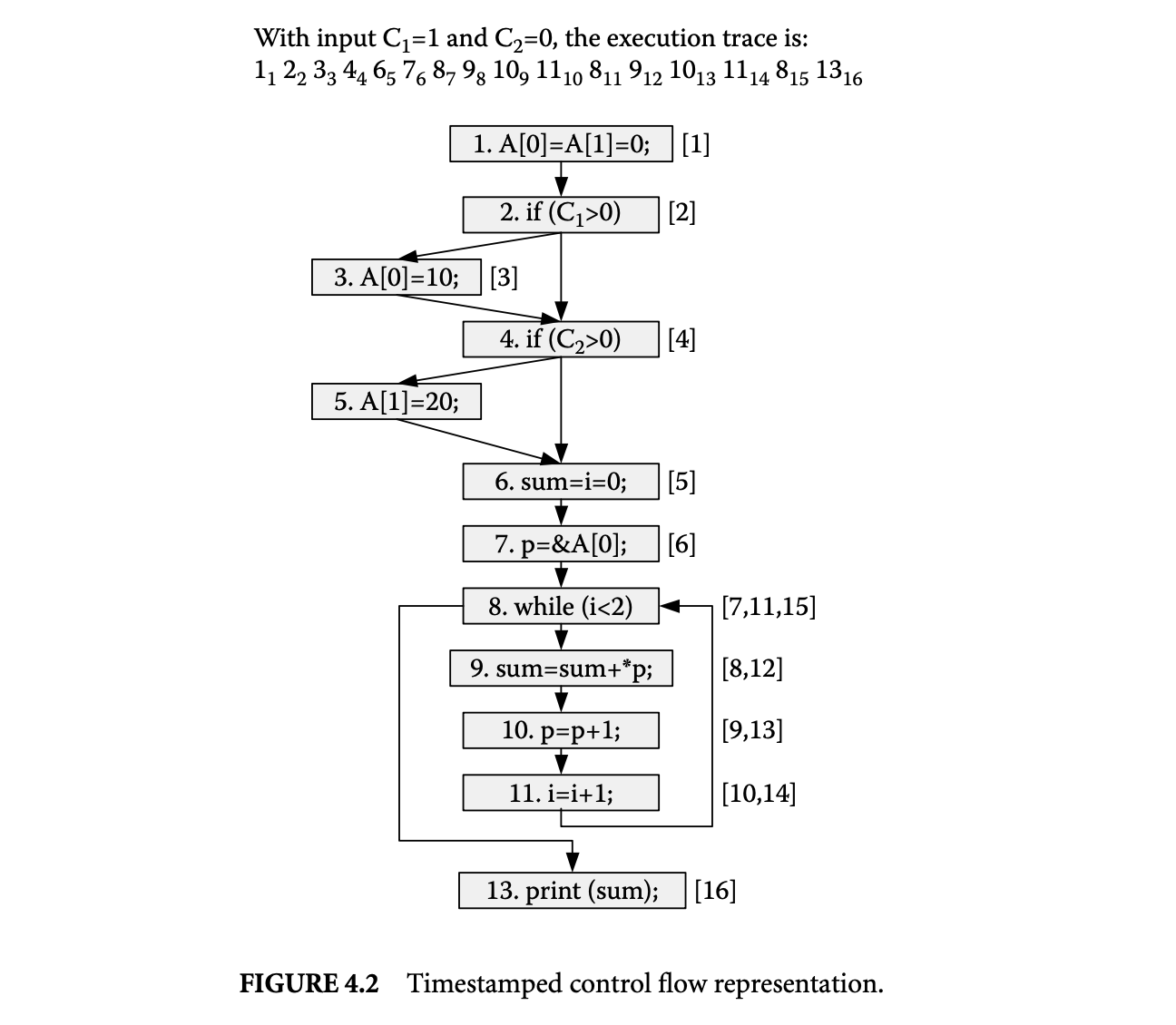
Let's see how the above timestamped representation captures the complete control flow trace. The path taken by the program can be generated from a labeled control flow graph using the combination of static control flow edges and the sequences of timestamps associated with nodes. If a node is labeled with timestamp value , the node that is executed next must be the static control flow successor of that is labeled with timestamp value . Using this observation, the complete path or part of the program path starting at any execution point can be easily generated.
4.2.1.2 Whole Value Trace
The whole value trace captures all values and addresses computed and referenced by executed statements. Instrumentation code must be introduced for each instruction in the program to collect the value trace for a program run. To represent the control flow trace, with each statement, we already associate a sequence of timestamps corresponding to the statement execution instances. To represent the value trace, we also associate a sequence of values with the statement. These are the values computed by the statement's execution instances. Hence, there is one-to-one correspondence between the sequence of timestamps and the sequence of values.
Two points are worth noting here. First, by capturing values as stated above, we are actually capturing both values and addresses, as some instructions compute data values while others compute addresses. Second, with each statement, we only associate the result values computed by that statement. We do not explicitly associate the values used as operands by the statement. This is because we can access the operand values by traversing the data dependence edges and then retrieving the values from the value traces of statements that produce these values.
Now let us illustrate the above representation by giving the value traces for the program run considered in Figure 4.2. The sequence of values produced by each statement for this program run is shown in Figure 4.3. For example, statement 11 is executed twice and produces values 1 and 2 during these executions.
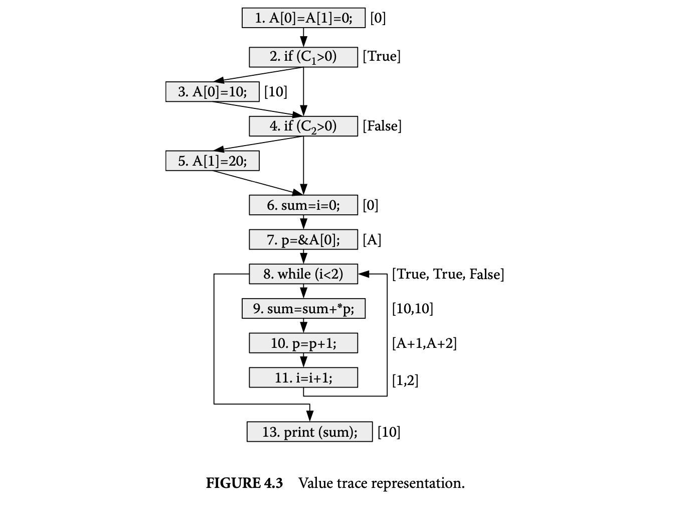
4.2.1.3 Whole Dependence Trace
A dependence occurs between a pair of statements; one is the source of the dependence and the other is the destination. Dependence is represented by an edge from the source to the destination in the static control flow graph. There are two types of dependences:
Static data dependence: A statement is statically data dependent upon statement if a value computed by statement may be used as an operand by statement in some program execution. Static control dependence: A statement is statically control dependent upon a predicate if the outcome of predicate can directly determine whether is executed in some program execution.
The whole data and control dependence trace captures the dynamic occurrences of all static data and control dependences during a program run. A static edge from the source of a dependence to its destination is labeled with dynamic information to capture each dynamic occurrence of a static dependence during the program run. The dynamic information essentially identifies the execution instances of the source and destination statements involved in a dynamic dependence. Since execution instances of statements are identified by their timestamps, each dynamic dependence is represented by a pair of timestamps that identify the execution instances of statements involved in the dynamic dependence. If a static dependence is exercised multiple times during a program run, it will be labeled by a sequence of timestamp pairs corresponding to multiple occurrences of the dynamic dependence observed during the program run.
Let us briefly discuss how dynamic dependences are identified during a program run. To identify dynamic data dependences, we need to further process the address trace. For each memory address the execution instance of an instruction that was responsible for the latest write to the address is remembered. When an execution instance of an instruction uses the value at an address, a dynamic data dependence is established between the execution instance of the instruction that performed the latest write to the address and the execution instance of the instruction that used the value at the address. Dynamic control dependences are also identified. An execution instance of an instruction is dynamically control dependent upon the execution instance of the predicate that caused the execution of the instruction. By first computing the static
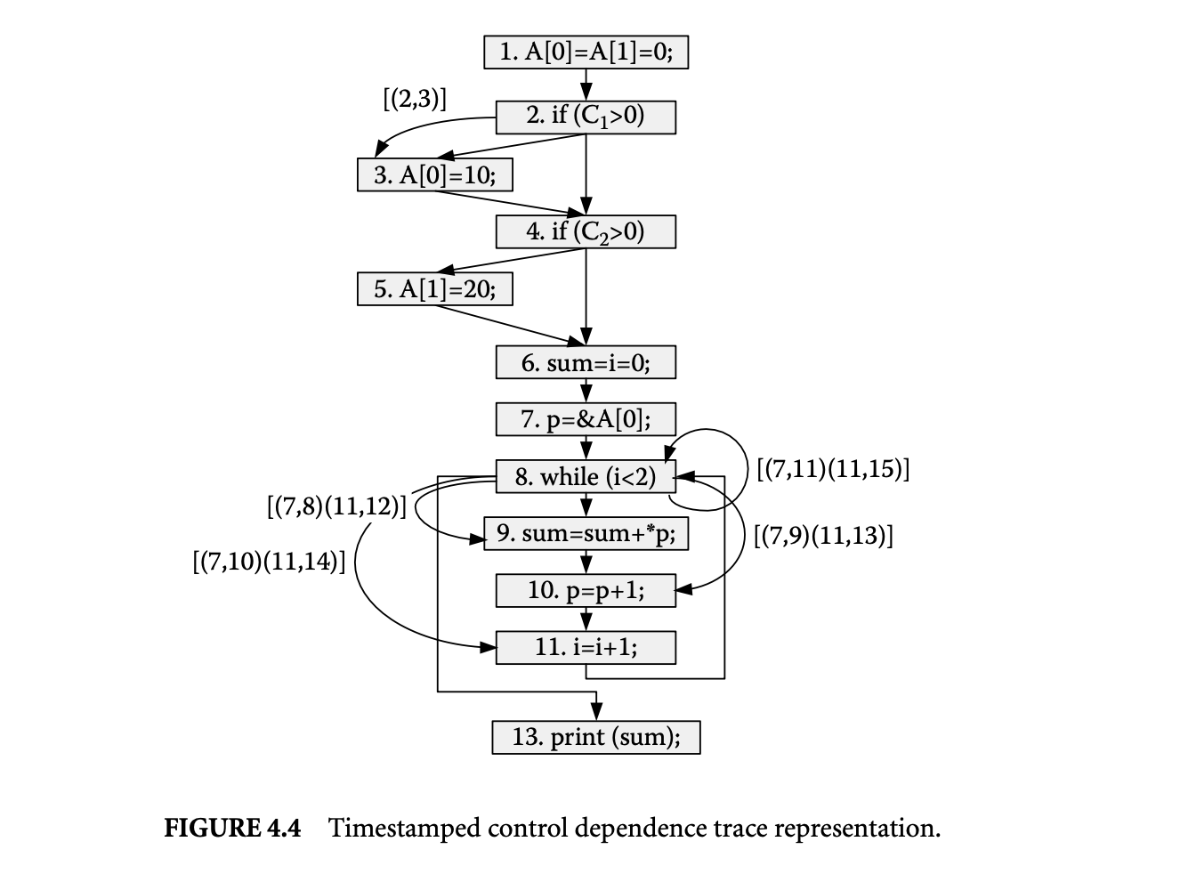
control predecessors of an instruction, and then detecting which one of these was the last to execute prior to a given execution of the instruction from the control flow trace, dynamic control dependences are identified.
Now let us illustrate the above representation by giving the dynamic data and control dependences for the program run considered in Figure 4.2. First let's consider the dynamic control dependences shown in Figure 4.4. The control dependence edges in this program include , , , , and . These edges are labeled with timestamp pairs. The edge is labeled with because this dependence is exercised only once and the timestamps of the execution instances involved are and . The edge is not labeled because it is not exercised in the program run. However, edge is labeled with , indicating that this edge is exercised twice. The timestamps in each pair identify the execution instances of statements involved in the dynamic dependences.
Next let us consider the dynamic data dependence edges shown in Figure 4.5. The darker edges correspond to static data dependence edges that are labeled with sequences of timestamp pairs that capture dynamic instances of data dependences encountered during the program run. For example, edge shows the flow of the value of variable from its definition in statement 11 to its use in statement 8. This edge is labeled because it is exercised twice in the program run. The timestamps in each pair identify the execution instances of statements involved in the dynamic dependences.
4.2.2 Compressing Whole Execution Traces
Because of the large amount of information contained in WETs, the storage needed to hold the WETs is very large. In this section we briefly outline a two-tier compression strategy for greatly reducing the space requirements.
The first tier of our compression strategy focuses on developing separate compression techniques for each of the three key types of information labeling the WET graph: (a) timestamps labeling the nodes, (b) values labeling the nodes, and (c) timestamp pairs labeling the dependence edges. Let us briefly consider these compression techniques:
Timestamps labeling the nodes: The total number of timestamps generated is equal to the number of basic block executions, and each of the timestamps labels exactly one basic block. We can reduce the
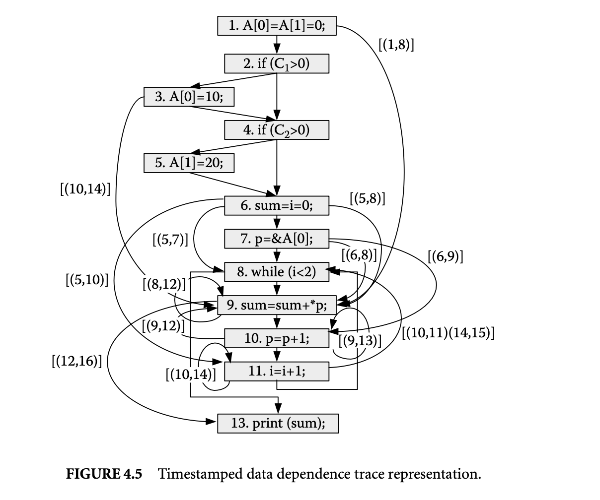 space taken up by the timestamp node labels as follows. Instead of having nodes that correspond to basic blocks, we create a WET in which nodes can correspond to Ball Larus paths [2] that are composed of multiple basic blocks. Since a unique timestamp value is generated to identify the execution of a node, now fewer timestamps will be generated. In other words, when a Ball Larus path is executed, all nodes in the path share the same timestamp. By reducing the number of timestamps, we save space without having any negative impact on the traversal of WET to extract the control flow trace.
Values labeling the nodes: It is well known that subcomputations within a program are often performed multiple times on the same operand values. This observation is the basis for widely studied techniques for reuse-based redundancy removal [18]. This observation can be exploited in devising a compression scheme for sequence of values associated with statements belonging to a node in the WET. The list of values associated with a statement is transformed such that only a list of unique values produced by it is maintained along with a pattern from which the exact list of values can be generated from the list of unique values. The pattern is often shared across many statements. The above technique yields compression because by storing the pattern only once, we are able to eliminate all repetitions of values in value sequences associated with all statements.
Timestamp pairs labeling the dependence edges:: Each dependence edge is labeled with a sequence of timestamp pairs. Next we describe how the space taken by these sequences can be reduced. Our discussion focuses on data dependences; however, similar solutions exist for handling control dependence edges [27]. To describe how timestamp pairs can be reduced, we divide the data dependences into two categories: edges that are local to a Ball Larus path and edges that are nonlocal as they cross Ball Larus path boundaries.
Let us consider a node that contains a pair of statements and such that a local data dependence edge exists due to flow of values from to . For every timestamp pair labeling the edge, it is definitely the case that . In addition, if always receives the involved operand value from , then we do not need to label this edge with timestamp pairs. This is because the timestamp pairs that label the edge can be inferred from the labels of node . If node is labeled with timestamp , under the above conditions,
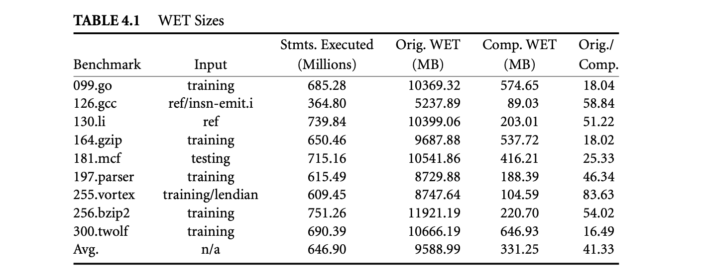
the data dependence edge must be labeled with the timestamp pair . It should be noted that by creating nodes corresponding to Ball Larus paths, opportunities for elimination of timestamp pair labels increase greatly. This is because many nonlocal edges get converted to local edges.
Let us consider nonlocal edges next. Often multiple data dependence edges are introduced between a pair of nodes. It is further often the case that these edges have identical labels. In this case we can save space by creating a representation for a group of edges and save a single copy of the labels.
For the second-tier compression we view the information labeling the WET as consisting of streams of values arising from the following sources: (a) a sequence of pairs labeling a node gives rise to two streams, one corresponding to the timestamps () and the other corresponding to the values (), and (b) a sequence of pairs labeling a dependence edge also gives rise to two streams, one corresponding to the first timestamps (s) and the other corresponding to the second timestamps (s). Each of the above streams is compressed using a value-prediction-based algorithm [28].
Table 1 lists the benchmarks considered and the lengths of the program runs, which vary from 365 and 751 million intermediate-level statements. WETs could not be collected for complete runs for most benchmarks even though we tried using Trimaran-provided inputs with shorter runs. The effect of our two-tier compression strategy is summarized in Table 1. While the average size of the original uncompressed WETs (Orig. WET) is 9589 megabytes, after compression their size (Comp. WET) is reduced to 331 megabytes, which represents a compression ratio (Orig./Comp.) of 41. Therefore, on average, our approach enables saving of the whole execution trace corresponding to a program run of 647 million intermediate statements using 331 megabytes of storage.
4.3 Using WET in Debugging
In this section we consider two debugging scenarios and demonstrate how WET-based analysis can be employed to assist in fault location in both scenarios. In the first scenario we have a program that fails to produce the correct output for a given input, and it is our goal to assist the programmer in locating the faulty code. In the second scenario we are given two versions of a program that should behave the same but do not do so on a given input, and our goal is to help the programmer locate the point at which the behavior of the two versions diverges. The programmer can then use this information to correct one of the versions.
4.3.1 Dynamic Program Slicing
Let us consider the following scenario for fault location. Given a failed run of a program, our goal is to identify a fault candidate set, that is, a small subset of program statements that includes the faulty code whose execution caused the program to fail. Thus, we assume that the fact that the program has failed is known because either the program crashed or it produced an output that the user has determined to be incorrect. Moreover, this failure is due to execution of faulty code and not due to other reasons (e.g., faulty environment variable setting).
The statements executed during the failing run can constitute a first conservative approximation of the fault candidate set. However, since the user has to examine the fault candidate set manually to locate faulty code, smaller fault candidate sets are desirable. Next we describe a number of dynamic-slicing-based techniques that can be used to produce a smaller fault candidate set than the one that includes all executed statements.
4.3.1.1 Backward Dynamic Slicing
Consider a failing run that produces an incorrect output value or crashes because of dereferencing of an illegal memory address. The incorrect output value or the illegal address value is now known to be related to faulty code executed during this failed run. It should be noted that identification of an incorrect output value will require help from the user unless the correct output for the test input being considered is already available to us. The fault candidate set is constructed by computing the backward dynamic slice starting at the incorrect output value or illegal address value. The backward dynamic slice of a value at a point in the execution includes all those executed statements that effect the computation of that value [1, 14]. In other words, statements that directly or indirectly influence the computation of faulty value through chains of dynamic data and/or control dependences are included in the backward dynamic slices. Thus, the backward reachable subgraph forms the backward dynamic slice, and all statements that appear at least once in the reachable subgraph are contained in the backward dynamic slice. During debugging, both the statements in the dynamic slice and the dependence edges that connect them provide useful clues to the failure cause.
We illustrate the benefit of backward dynamic slicing with an example of a bug that causes a heap overflow error. In this program, a heap buffer is not allocated to be wide enough, which causes an overflow. The code corresponding to the error is shown in Figure 4.6. The heap array allocated at line 10 overflows at line 11, causing the program to crash. Therefore, the dynamic slice is computed starting at the address of that causes the segmentation fault. Since the computation of the address involves and , both statements at lines 10 and 10 are included in the dynamic slice. By examining statements at lines 10 and 10, the cause of the failure becomes evident to the programmer. It is easy to see that although a_count entries have been allocated at line 10, b_count entries are accessed according to the loop bounds of the for statement at line 10. This is the cause of the heap overflow at line 11. The main benefit of using dynamic slicing is that it focuses the attention of the programmer on the two relevant lines of code (10 and 10), enabling the fault to be located.
We studied the execution times of computing backward dynamic slices using WETs. The results of this study are presented in Figure 4.7. In this graph each point corresponds to the average dynamic slicing time for 25 slices. For each benchmark 25 new slices are computed after an execution interval of 15 million statements. These slices correspond to 25 distinct memory references. Following each execution interval slices are computed for memory addresses that had been defined since the last execution interval. This was done to avoid repeated computation of the same slices during the experiment. The increase in slicing times is linear with respect to the number of statements executed. More importantly, the slicing times are very promising. For 9 out of 10 benchmarks the average slicing time for 25 slices computed at the end of the run is below 18 seconds. The only exception is 300.twolf, for which the average slicing time at the
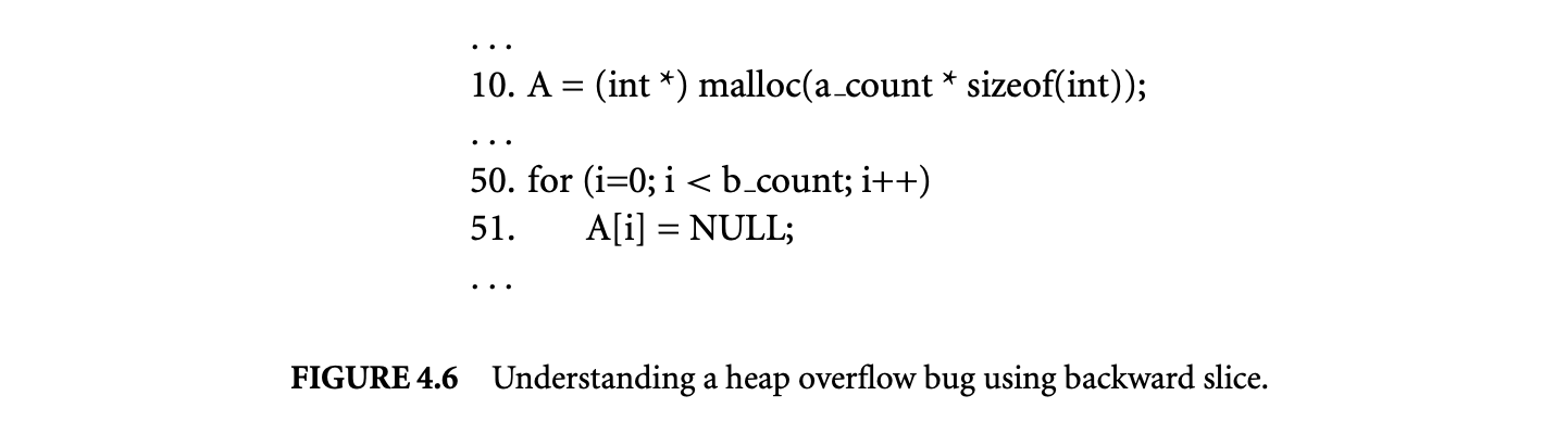
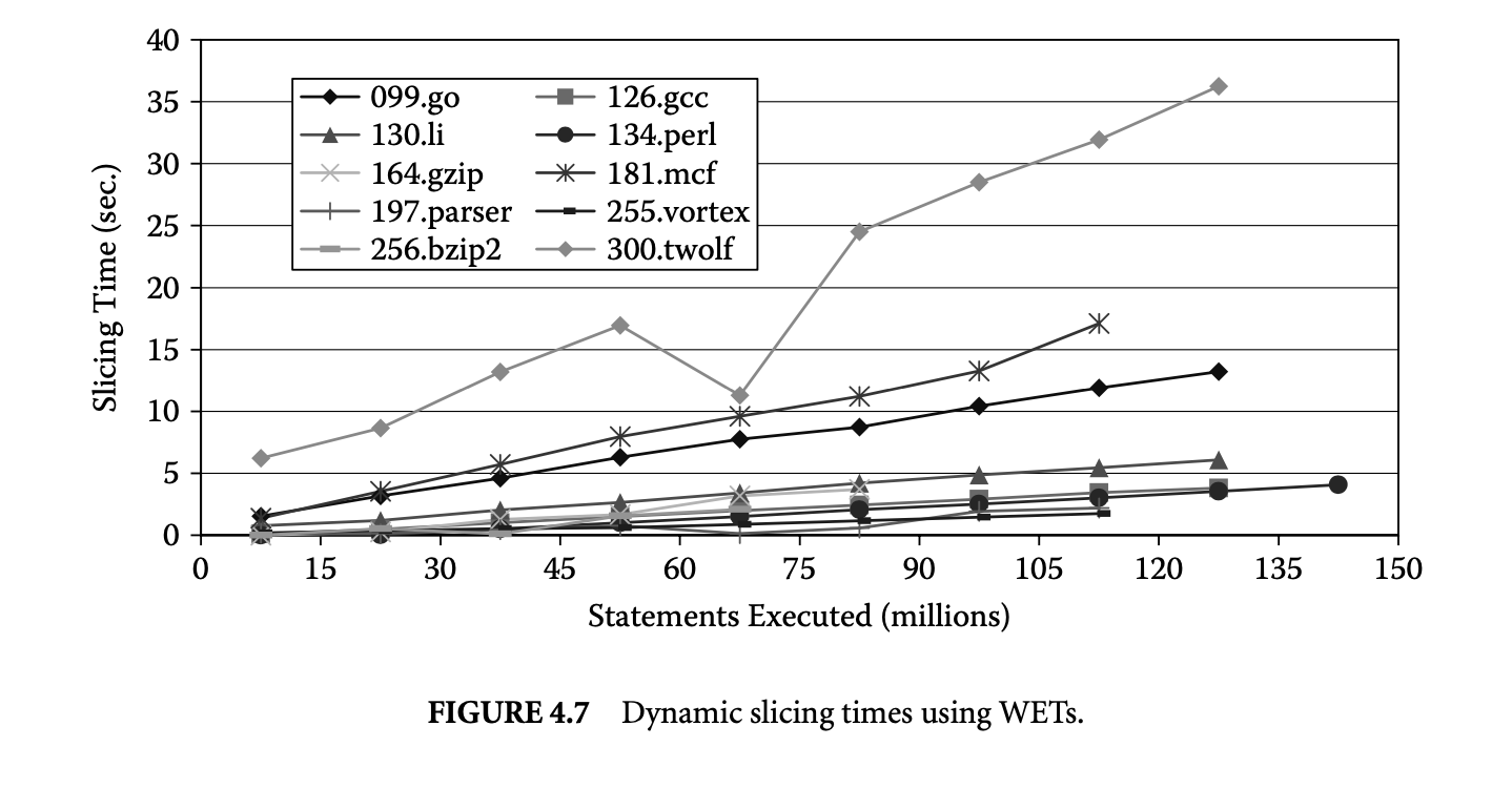 end of the program run is roughly 36 seconds. We noted that the compression algorithm did not reduce the graph size for this program as much as many of the other benchmarks. Finally, at earlier points during program runs the slicing times are even lower.
4.3.1.2 Forward Dynamic Slicing
Zeller introduced the term delta debugging[22] for the process of determining the causes of program behavior by looking at the differences (the deltas) between the old and new configurations of the programs. Hildebrandt and Zeller [10, 23] then applied the delta debugging approach to simplify and isolate the failure-inducing input difference. The basic idea of delta debugging is as follows. Given two program runs and corresponding to the inputs and , respectively, such that the program fails in run and completes execution successfully in run , the delta debugging algorithm can be used to systematically produce a pair of inputs and with a minimal difference such that the program fails for and executes successfully for . The difference between these two inputs isolates the failure-inducing difference part of the input. These inputs are such that their values play a critical role in distinguishing a successful run from a failing run.
Since the minimal failure-inducing input difference leads to the execution of faulty code and hence causes the program to fail, we can identify a fault candidate set by computing a forward dynamic slice starting at this input. In other words, all statements that are influenced by the input value directly or indirectly through a chain of data or control dependences are included in the fault candidate set. Thus, now we have a means for producing a new type of dynamic slice that also represents a fault candidate set. We recognized the role of forward dynamic slices in fault location for the first time in [8].
Let us illustrate the use of forward dynamic slicing using the program in Figure 4.8. In this program if the length of the input is longer than 1,024, the writes to Buffer[i] at line 6 overflow the buffer corrupting the pointer stored in CorruptPointer. As a result, when we attempt to execute the free at line 9, the program crashes.
Let us assume that to test the above program we picked the following two inputs: the first input is 'aaaaa', which is a successful input, and the second input is 'a repeated 2000 times , which is a failing input because the length is larger than 1,024. After applying the algorithm in [23] on them, we have two new inputs: the new successful input is 'a repeated 1024 times and the new failing input is 'a repeated 1025 times . The failure-inducing input difference between them is the last character 'a' in the new failed input.
Now we compute the forward dynamic slice of 1,025th 'a' in the failing input. The resulting dynamic slice consists of a data dependence chain originating at statement INPUT[i] at line 5, leading to the write to
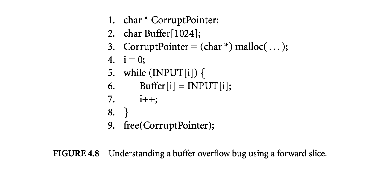 Buffer[i] at line 6, and then leading to the statement free(CorruptPointer) at line 9. When the programmer examines this data dependence chain, it becomes quite clear that there is an unexpected data dependence from Buffer[i] at line 6 to free(CorruptPointer) at line 9. Therefore, the programmer can conclude that Buffer[i] has overflowed. This is the best result one can expect from a fault location algorithm. This is because, other than the input statement, the forward dynamic slice captures exactly two statements. These are the two statements between which the spurious data dependence was established, and hence they must be minimally present in the fault candidate set.
4.3.1.3 Bidirectional Dynamic Slicing
Given an erroneous run of the program, the objective of this method is to explicitly force the control flow of the program along an alternate path at a critical branch predicate such that the program produces the correct output. The basic idea of this approach is inspired by the following observation. Given an input on which the execution of a program fails, a common approach to debugging is to run the program on this input again, interrupt the execution at certain points to make changes to the program state, and then see the impact of changes on the continued execution. If we can discover the changes to the program state that cause the program to terminate correctly, we obtain a good idea of the error that otherwise was causing the program to fail. However, automating the search of state changes is prohibitively expensive and difficult to realize because the search space of potential state changes is extremely large (e.g., even possible changes for the value of a single variable are enormous if the type of the variable is integer or float). However, changing the outcomes of predicate instances greatly reduces the state search space since a branch predicate has only two possible outcomes: true or false. Therefore, we note that through forced switching of the outcomes of some predicate instances at runtime, it may be possible to cause the program to produce correct results.
Having identified a critical predicate instance, we compute a fault candidate set as the bidirectional dynamic slice of the critical predicate instance. This bidirectional dynamic slice is essentially the union of the backward dynamic slice and the forward dynamic slice of the critical predicate instance. Intuitively, the reason the slice must include both the backward and forward dynamic slice is as follows. Consider the situation in which the effect of executing faulty code is to cause the predicate to evaluate incorrectly. In this case the backward dynamic slice of the critical predicate instance will capture the faulty code. However, it is possible that by changing the outcome of the critical predicate instance we avoid the execution of faulty code, and hence the program terminates normally. In this case the forward dynamic slice of the critical predicate instance will capture the faulty code. Therefore, the faulty code will be in either the backward dynamic slice or the forward dynamic slice. We recognized the role of bidirectional dynamic slices in fault location for the first time in [26], where more details on identification of the critical predicate instance can also be found.
Next we present an example to illustrate the need for bidirectional dynamic slices. We consider a simple program shown in Figure 4.9 that sums up the elements of an array . While this is the correct version of the program, next we will create three faulty versions of this program. In each of these versions the critical predicate instance can be found. However, the difference in these versions is where in the bidirectional dynamic slice the faulty code is present,
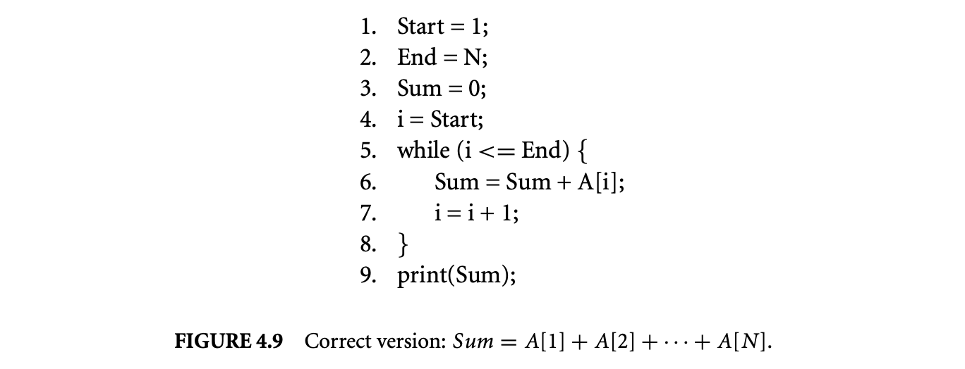 that is, the critical predicate, the backward dynamic slice of the critical predicate, and the forward dynamic slice of the critical predicate:
Fault in the critical predicate:: Figure 4.10 shows a faulty version of the program from Figure 4.9. In this faulty version, the error in the predicate of the while loop results in the loop executing for one fewer iterations. As a result, the value of is not added to Sum, producing an incorrect output. The critical predicate instance identified for this program run is the last execution instance of the while loop predicate. This is because if the outcome of the last execution instance of the while loop predicate is switched from false to true, the loop iterates for another iteration and the output produced by the program becomes correct. Given this information, the programmer can ascertain that the error is in the while loop predicate, and it can be corrected by modifying the relational operator from to .
Fault in the backward dynamic slice of the critical predicate instance:: In the previous faulty version, the critical predicate identified was itself faulty. Next we show that in a slightly altered version of the faulty version, the fault is not present in the critical predicate but rather in the backward dynamic slice of the critical predicate. Figure 4.11 shows this faulty version. The fault is in the initialization of End at line 3, and this causes the while loop to execute for one fewer iterations. Again, the value of is not added to Sum, producing an incorrect output. The critical predicate instance identified for this program run is the last execution instance of the while loop predicate. This is because if the outcome of the last execution instance of the while loop predicate is switched from false to true, the loop iterates for another iteration and the output produced by the program becomes correct. However, in this situation the programmer must examine the backward dynamic slice of the critical predicate to locate the faulty initialization of End at line 3.
Fault in the forward dynamic slice of the critical predicate instance:: Finally, we show a faulty version in which the faulty code is present in the forward dynamic slice of the critical predicate instance. Figure 4.12 shows this faulty version. The fault is at line 6, where reference to should bereplaced by reference to .
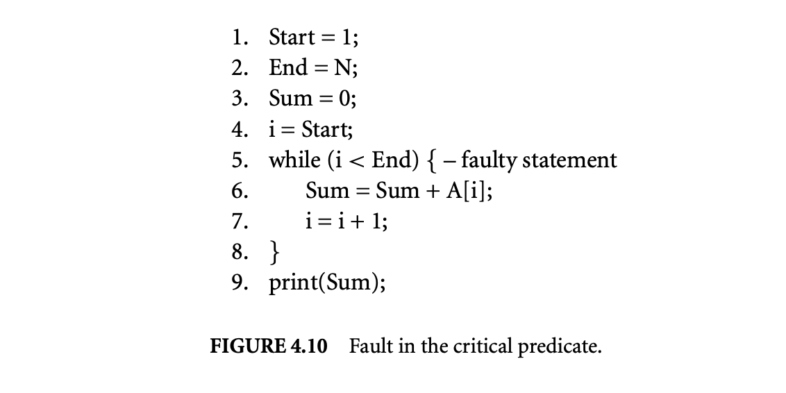
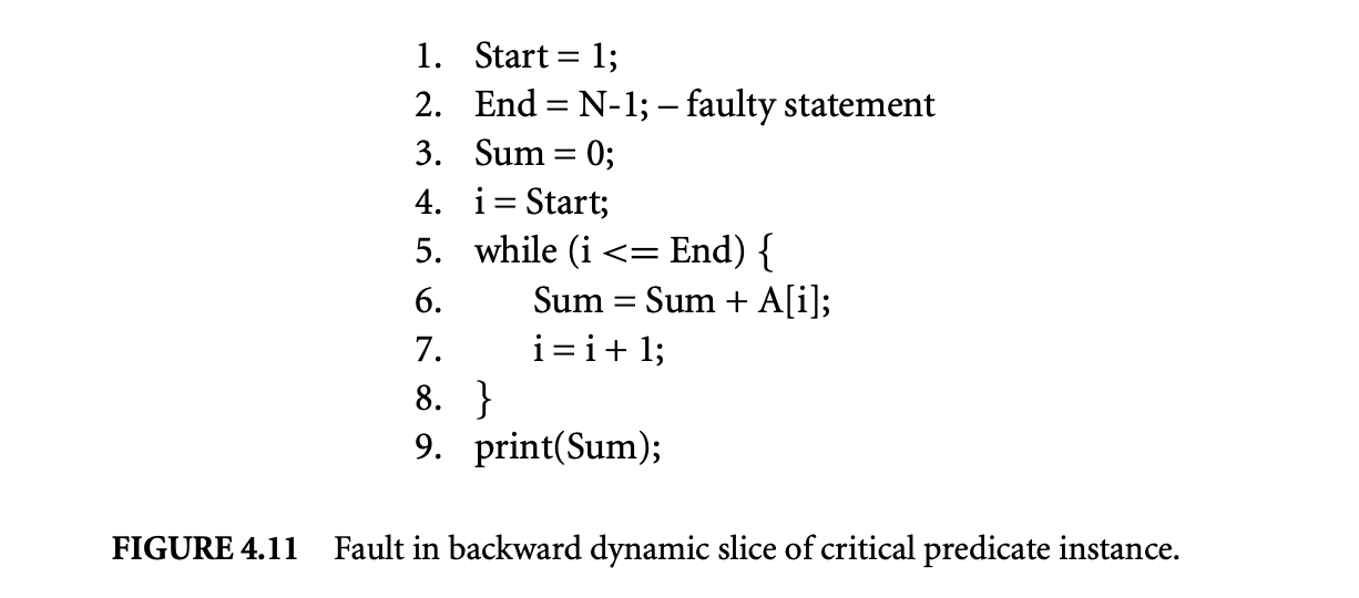
When this faulty version is executed, let us consider the situation in which when the last loop iteration is executed, the reference to at line 6 causes the program to produce a segmentation fault. The most recent execution instance of the while loop predicate is evaluated to true. However, if we switch this evaluation to false, the loop executes for one fewer iterations, causing the program crash to disappear. Note that the output produced is still incorrect because the value of is not added to Sum. However, since the program no longer crashes, the programmer can analyze the program execution to understand why the program crash is avoided. By examining the forward dynamic slice of the critical predicate instance, the programmer can identify the statements, which when not executed avoid the program crash. This leads to the identification of reference to as the fault.
In the above discussion we have demonstrated that once the critical predicate instance is found, the fault may be present in the critical predicate, its backward dynamic slice, or its forward dynamic slice. Of course, the programmer does not know beforehand where the fault is. Therefore, the programmer must examine the critical predicate, the statements in the backward dynamic slice, and the statements in the forward dynamic slice one by one until the faulty statement is found.
4.3.1.4 Pruning Dynamic Slices
In the preceding discussion we have shown three types of dynamic slices that represent reduce fault candidate sets. In this section we describe two additional techniques for further pruning the sizes of the fault candidate sets:
Coarse-grained pruning:: When multiple estimates of fault candidate sets are found using backward, forward, and bidirectional dynamic slices, we can obtain a potentially smaller fault candidate set by intersecting the three slices. We refer to this simple approach as the coarse-grained pruning approach. In [24] we demonstrate the benefits of this approach by applying it to a collection of real bugs reported by users. The results are very encouraging, as in many cases the fault candidate set contains only a handful of statements.
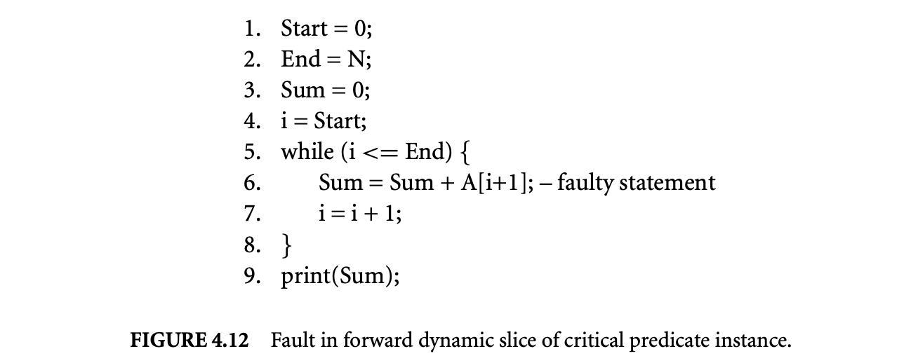 Fine-grained pruning: In general, it is not always possible to compute fault candidate sets using backward, forward, and bidirectional dynamic slices. For example, if we fail to identify a minimal failure-inducing input difference and a critical predicate instance, then we cannot compute the forward and bidirectional dynamic slices. As a result, coarse-grained pruning cannot be applied. To perform pruning in such situations we developed a fine-grained pruning technique that reduces the fault candidate set size by eliminating statements in the backward dynamic slice that are expected not to be faulty.
The fine-grained pruning approach is based upon value profiles of executed statements. The main idea behind this approach is to exploit correct outputs produced during a program run before an incorrect output is produced or the program terminates abnormally. The executed statements and their value profiles are examined to find likely correct statements in the backward slice. These statements are such that if they are altered, they will definitely cause at least one correct output produced during the program run to change. All statements that fall in this category are marked as likely correct and thus pruned from the backward dynamic slice. The detailed algorithm can be found in [25] along with experimental data that show that this pruning approach is highly effective in reducing the size of the fault candidate set. It should be noted that this fine-grained pruning technique makes use of both dependence and value traces contained in the WET.
4.3.2 Dynamic Matching of Program Versions
Now we consider a scenario in which we have two versions of a program such that the second version has been derived through application of transformations to the first version. When the two versions are executed on an input, it is found that while the first version runs correctly, the second version does not. In such a situation it is useful to find out the execution point at which the dynamic behavior of the two versions deviates, since this gives us a clue to the cause of differing behaviors.
The above scenario arises in the context of optimizing compilers. Although compile-time optimizations are important for improving the performance of programs, applications are typically developed with the optimizer turned off. Once the program has been sufficiently tested, it is optimized prior to its deployment. However, the optimized program may fail to execute correctly on an input even though the unoptimized program ran successfully on that input. In this situation the fault may have been introduced by the optimizer through the application of an unsafe optimization, or a fault present in the original program may have been exposed by the optimizations. Determining the source and cause of the fault is therefore important.
In [12] a technique called comparison checking was proposed to address the above problem. A comparison checker executes the optimized and unoptimized programs and continuously compares the results produced by corresponding instruction executions from the two versions. At the earliest point during execution at which the results differ, they are reported to the programmer, who can use this information to isolate the cause of the faulty behavior. It should be noted that not every instruction in one version has a corresponding instruction in the other version because optimizations such as reassociation may lead to instructions that compute different intermediate results. While the above approach can be used to test optimized code thoroughly and assist in locating a fault if one exists, it has one major drawback. For the comparison checker to know which instruction executions in the two versions correspond to each other, the compiler writer must write extra code that determines mappings between execution instances of instructions in the two program versions. Not only do we need to develop a mapping for each kind of optimization to capture the effect of that optimization, but we must also be able to compose the mappings for different optimizations to produce the mapping between the unoptimized and fully optimized code. The above task is not only difficult and time consuming, but it must be performed each time a new optimization is added to the compiler.
We have developed a WET-based approach for automatically generating the mappings. The basic idea behind our approach is to run the two versions of the programs and regularly compare their execution histories. The goal of this comparison is to find matches between the execution history of each instruction in the optimized code with execution histories of one or more instructions in the unoptimized code.
If execution histories match closely, it is extremely likely that they are indeed the corresponding instructions in the two program versions. At each point when executions of the programs are interrupted, their histories are compared with each other. Following the determination of matches, we determine if faulty behavior has already manifested itself, and accordingly potential causes of faulty behavior are reported to the user for inspection. For example, instructions in the optimized program that have been executed numerous times but do not match anything in the unoptimized code can be reported to the user for examination. In addition, instructions that matched each other in an earlier part of execution but later did not match can be reported to the user. This is because the later phase of execution may represent instruction executions after faulty behavior manifests itself. The user can then inspect these instructions to locate the fault(s).
The key problem we must solve to implement the above approach is to develop a matching process that is highly accurate. We have designed a WET-based matching algorithm that consists of the following two steps: signature matching and structure matching. A signature of an instruction is defined in terms of the frequency distributions of the result values produced by the instruction and the addresses referenced by the instruction. If signatures of two instructions are consistent with each other, we consider them to tentatively match. In this second step we match the structures of the data dependence graphs produced by the two versions. Two instructions from the two versions are considered to match if there was a tentative signature match between them and the instructions that provided their operands also matched with each other.
In the Trimaran system [19] we generated two versions of very long instructional word (VIW) machine code supported under the Trimaran system by generating an unoptimized and an optimized version of programs. We ran the two versions on the same input and collected their detailed whole execution traces. The execution histories of corresponding functions were then matched. We found that our matching algorithm was highly accurate and produced the matches in seconds [29]. To study the effectiveness of matching for comparison checking as discussed above, we created another version of the optimized code by manually injecting an error in the optimized code. We plotted the number of distinct instructions for which no match was found as a fraction of distinct executed instructions over time in two situations: when the optimized program had no error and when it contained an error. The resulting plot is shown in Figure 4.13. The points in the graph are also annotated with the actual number of instructions in the optimized code for which no match was found. The interval during which an error point is encountered during execution is marked in the figure.
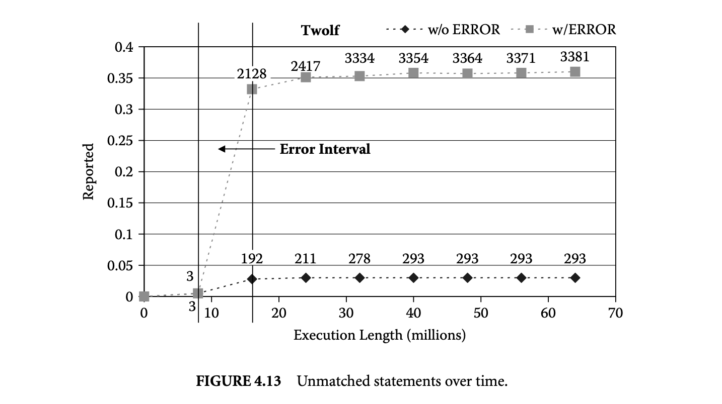
Compared to the optimized program without error, the number of unmatched instructions increases sharply after the error interval point is encountered. The increase is quite sharp -- from 3 to 35%. When we look at the actual number of instructions reported immediately before and after the execution interval during which the error is first encountered, the number reported increases by an order of magnitude.
By examining the instructions in the order they are executed, erroneous instructions can be quickly isolated. Other unmatched instructions are merely dependent upon the instructions that are the root causes of the errors. Out of the over 2,000 unmatched instructions at the end of the second interval, we only need to examine the first 15 unmatched instructions in temporal order to find an erroneous instruction.
4.4 Concluding Remarks
The emphasis of earlier research on profiling techniques was separately studying single types of profiles (control flow, address, value, or dependence) and capturing only a subset of profile information of a given kind (e.g., hot control flow paths, hot data streams). However, recent advances in profiling enable us to simultaneously capture and compactly represent complete profiles of all types. In this chapter we described the WET representation that simultaneously captures complete profile information of several types of profile data. We demonstrated how such rich profiling data can serve as the basis of powerful dynamic analysis techniques. In particular, we described how dynamic slicing and dynamic matching can be performed efficiently and used to greatly assist a programmer in locating faulty code under two debugging scenarios.
References
- H. Agrawal and J. Horgan. 1990. Dynamic program slicing. In ACM SIGPLAN Conference on Programming Language Design and Implementation, 246-56. New York, NY: ACM Press.
- T. Ball and J. Larus. 1996. Efficient path profiling. In IEEE/ACM International Symposium on Microarchitecture, 46-57. Washington, DC, IEEE Computer Society.
- R. Bodik, R. Gupta, and M. L. Soffa. 1998. Complete removal of redundant expressions. In ACM SIGPLAN Conference on Programming Language Design and Implementation, 1-14, Montreal, Canada. New York, NY: ACM Press.
- M. Burtscher and M. Jeeradit. 2003. Compressing extended program traces using value predictors. In International Conference on Parallel Architectures and Compilation Techniques, 159-69. Washington, DC, IEEE Computer Society.
- B. Calder, P. Feller, and A. Eustace. 1997. Value profiling. In IEEE/ACM International Symposium on Microarchitecture, 259-69. Washington, DC, IEEE Computer Society.
- T. M. Chilimbi. 2001. Efficient representations and abstractions for quantifying and exploiting data reference locality. In ACM SIGPLAN Conference on Programming Language Design and Implementation, 191-202, Snowbird, UT. New York, NY: ACM Press.
- T. M. Chilimbi and M. Hirzel. 2002. Dynamic hot data stream prefetching for general-purpose programs. In ACM SIGPLAN Conference on Programming Language Design and Implementation, 199-209. New York, NY: ACM Press.
- N. Gupta, H. He, X. Zhang, and R. Gupta. 2005. Locating faulty code using failure-inducing chops. In IEEE/ACM International Conference on Automated Software Engineering, 263-72, Long Beach, CA. New York, NY: ACM Press.
- R. Gupta, D. Berson, and J. Z. Fang. 1998. Path profile guided partial redundancy elimination using speculation. In IEEE International Conference on Computer Languages, 230-39, Chicago, IL. Washington, DC, IEEE Computer Society.
- R. Hildebrandt and A. Zeller. 2000. Simplifying failure-inducing input. In International Symposium on Software Testing and Analysis, 135-45. New York, NY: ACM Press.
- Q. Jacobson, E. Rotenberg, and J. E. Smith. 1997. Path-based next trace prediction. In IEEE/ACM International Symposium on Microarchitecture, 14-23. Washington, DC, IEEE Computer Society.
- C. Jaramillo, R. Gupta, and M. L. Soffa. 1999. Comparison checking: An approach to avoid debugging of optimized code. In ACM SIGSOFT 7th Symposium on Foundations of Software Engineering and 8th European Software Engineering Conference. LNCS 1687, 268-84. Heidelberg, Germany: Springer-Verlag. New York, NY: ACM Press.
- D. Joseph and D. Grunwald. 1997. Prefetching using Markov predictors. In International Symposium on Computer Architecture, 252-63. New York, NY: ACM Press.
- B. Korel and J. Laski. 1988. Dynamic program slicing. Information Processing Letters, 29(3): 155-63. Amsterdam, The Netherlands: Elsevier North-Holland, Inc.
- J. R. Larus. 1999. Whole program paths. In ACM SIGPLAN Conference on Programming Language Design and Implementation, 259-69, Atlanta, GA. New York, NY: ACM Press.
- M. H. Lipasti and J. P. Shen. 1996. Exceeding the dataflow limit via value prediction. In IEEE/ACM International Symposium on Microarchitecture, 226-37. Washington, DC, IEEE Computer Society.
- S. Rubin, R. Bodik, and T. Chilimbi. 2002. An efficient profile-analysis framework for data layout optimizations. In ACM SIGPLAN-SIGACT Symposium on Principles of Programming Languages, 140-53, Portland, OR. New York, NY: ACM Press.
- Y. Sazeides. 2003. Instruction-isomorphism in program execution. Journal of Instruction Level Parallelism, 5:1-22.
- L. N. Chakrapani, J. Gyllenhaal, W. Hwu, S. A. Mahlke, K. V. Palem, and R. M. Rabbah, Trimaran: An infrastructure for research in instruction-level parallelism, languages, and compliers for high performance computing 2004, LNCS 8602, 32-41, Berlin: Springer/Heidlberg.
- J. Yang and R. Gupta. 2002. Frequent value locality and its applications. ACM Transactions on Embedded Computing Systems, 1(1):79-105. New York, NY: ACM Press.
- C. Young and M. D. Smith. 1998. Better global scheduling using path profiles. In IEEE/ACM International Symposium on Microarchitecture, 115-23. Washington, DC, IEEE Computer Society.
- A. Zeller. 1999. Yesterday, my program worked. Today, it does not. Why? In ACM SIGSOFT Seventh Symposium on Foundations of Software Engineering and Seventh European Software Engineering Conference, 253-67. New York, NY: ACM Press.
- A. Zeller and R. Hildebrandt. 2002. Simplifying and isolating failure-inducing input. IEEE Transactions on Software Engineering, 28(2):183-200. Washington, DC, IEEE Computer Society.
- Practice & Experience_, vol 37, Issue 9, pp. 935-961, July 2007. New York, NY: John Wiley & Sons, Inc.
- X. Zhang, N. Gupta, and R. Gupta. 2006. Pruning dynamic slices with confidence. In ACM SIGPLAN Conference on Programming Language Design and Implementation, 169-80, Ottawa, Canada. New York, NY: ACM Press.
- X. Zhang, N. Gupta, and R. Gupta. 2006. Locating faults through automated predicate switching. In International Conference on Software Engineering, 272-81, Shanghai, China. New York, NY: ACM Press.
- X. Zhang and R. Gupta. 2004. Cost effective dynamic program slicing. In ACM SIGPLAN Conference on Programming Language Design and Implementation, 94-106, Washington, DC. New York, NY: ACM Press.
- X. Zhang and R. Gupta. 2005. Whole execution traces and their applications. ACM Transactions on Architecture and Code Optimization, 2(3):301-34. New York, NY: ACM Press.
- X. Zhang and R. Gupta. 2005. Matching execution histories of program versions. In Joint 10th European Software Engineering Conference and ACM SIGSOFT 13th Symposium on Foundations of Software Engineering, 197-206, Lisbon, Portugal. New York, NY: ACM Press.
- Y. Zhang and R. Gupta. 2001. Timestamped whole program path representation and its applications. In ACM SIGPLAN Conference on Programming Language Design and Implementation, 180-90, Snowbird, UT. New York, NY: ACM Press.
- Y. Zhang and R. Gupta. 2002. Data compression transformations for dynamically allocated data structures. In International Conference on Compiler Construction, Grenoble, France. London, UK: Springer-Verlag.
- C. B. Zilles and G. Sohi. 2000. Understanding the backward slices of performance degrading instructions. In ACM/IEEE 27th International Symposium on Computer Architecture, 172-81. New York, NY: ACM Press.
Chapter 5. Optimizations for Memory Hierarchies
5.1 Introduction
Since the advent of microprocessors, the clock speeds of CPUs have increased at an exponential rate. While the speed at which off-chip memory can be accessed has also increased exponentially, it has not increased at the same rate. A memory hierarchy is used to bridge this gap between the speeds of the CPU and the memory. In a memory hierarchy, the off-chip main memory is at the bottom. Above it, one or more levels of memory reside. Each level is faster than the level below it but stores a smaller amount of data. Sometimes registers are considered to be the topmost level of this hierarchy.
There are two ways in which the intermediate levels of this hierarchy can be organized.
The most popular approach, used in most general-purpose processors, is to use cache memory. A cache contains some frequently accessed subset of the data in the main memory. When the processor wants to access a piece of data, it first checks the topmost level of the hierarchy and goes down until the data sought is found. Most current processors have either two or three levels of caches on top of the main memory. Typically, the hardware controls which subset of state of one level is stored in a higher level. In a cache-based memory hierarchy, the average time to access a data item depends upon the probability of finding the data at each level of the hierarchy. Embedded systems use scratch pad memory in their memory subsystems. Scratch pads are smaller and faster addressable memory spaces. The compiler or the programmer directs where each data item should reside. In this chapter, we restrict our attention to cache-based memory hierarchies. This chapter discusses compiler transformations that reduce the average access latency of accessing data and instructions from memory. The average latency of accesses can be reduced in several ways. The first approach is to reduce the number of cache misses. There are three types of cache misses. Cold misses are the misses that are seen when a data item is accessed for the first time in the program and hence is not found in the cache. Capacity misses are caused when the current working set of the program is greater than the size of the cache. Conflict misses happen when more than one data item maps to the same cache line, thereby evicting some data in the current working set from the cache, but the current working set itself fits within the cache. The second approach is to reduce the average number of cycles needed to service a cache miss. The optimizations discussed later in this chapter reduce the average access latency by reducing the cache misses, by minimizing the access latency on a miss, or by a combination of both. In many processor architectures, the compiler cannot explicitly specify which data items should be placed at each level of the memory hierarchy. Even in architectures that support such directives, the hardware still maintains primary control. In either case, the compiler performs various transformations to reduce the access latency:
- Code restructuring optimizations: The order in which data items are accessed highly influences which set of data items are available in a given level of cache hierarchy at any given time. In many cases, the compiler can restructure the code to change the order in which data items are accessed without altering the semantics of the program. Optimizations in this category include loop interchange, loop blocking or tiling, loop skewing, loop fusion, and loop fission.
- Prefetching optimizations: Some architectures do provide support in the instruction set that allows the compiler some explicit control of what data should be in a particular level of the hierarchy. This is typically in the form of prefetch instructions. As the name suggests, a prefetch instruction allows a data item to be brought into the upper levels of the hierarchy before the data is actually used by the program. By suitably inserting such prefetch instructions in the code, the compiler can decrease the average data access latency.
- Data layout optimizations: All data items in a program have to be mapped to addresses in the virtual address space. The mapping function is often irrelevant to the correctness of the program, as long as two different items are with overlapping lifetimes not mapped to overlapping address ranges. However, this can have an effect on which level of the hierarchy a data item is found and hence on the execution time. Optimizations in this category include structure splitting, structure peeling, and stack, heap, and global data object layout.
- Code layout optimizations: The compiler has even more freedom in mapping instructions to address ranges. Code layout optimizations use this freedom to ensure that most of the code is found in the topmost level of the instruction cache.
While the compiler can optimize for the memory hierarchies in many ways, it also faces some significant challenges. The first challenge is in analyzing and understanding memory access patterns of applications. While significant progress has been made in developing better memory analyses, there remain many cases where the compiler has little knowledge of the memory behavior of applications. In particular, irregular access patterns such as traversals of linked data structures still thwart memory optimization efforts on the part of modern compilers. Indeed, most of the optimizations for memory performance are designed to handle regular access patterns such as strided array references. The next challenge comes from the fact that many optimizations for memory hierarchies are highly machine dependent. Incorrect assumptions about the underlying memory hierarchy often reduce the benefits of these optimizations and may even degrade the performance. An optimization that targets a cache with a line size of 64 bytes may not be suitable for processors with a cache line size of 128 bytes. Thus, the compiler needs to model the memory hierarchy as accurately as possible. This is a challenge given the complex memory subsystem found in modern processors. In Intel's Itanium, for example, the miss latency of first-level and second-level caches depends upon on factors such as the occupancy of the queue that contains the requests to the second-level cache. Despite these difficulties, memory optimizations are worthwhile, given how much memory behavior dictates overall program performance.
The rest of this chapter is organized as follows. Section 5.2 provides some background on the notion of dependence within loops and on locality analysis that is needed to understand some of the optimizations. Sections 5.3, 5.4, and 5.5 discuss some code restructuring optimizations. Section 5.6 deals with data prefetching, and data layout optimizations are discussed in Section 5.7. Optimizations for the instruction cache are covered in Section 5.8. Section 5.9 briefly summarizes the optimizations and discusses some future directions, and Section 5.10 discusses references to various works in this area.
5.2 Background
Code restructuring and data prefetching optimizations typically depend on at least partial regularity in data access patterns. Accesses to arrays within loops are often subscripted by loop indices, resulting in very regular patterns. As a result, most of these techniques operate at the granularity of loops. Hence, we first present some theory on loops that will be used in subsequent sections. A different approach to understanding loop accesses by using the domain of -polyhedra to model the loop iteration space is discussed by Rajopadhye et al. [24].
5.2.1 Dependence in Loops
Any compiler transformation has to preserve the semantics of the original code. This is ensured by preserving all true dependences in the original code. Traditional definitions of dependence between instructions are highly imprecise when applied to loops. For example, consider the loop in Figure 5.1 that computes the row sums of a matrix. By the traditional definition of true dependence, the statement row_sum[i]+= matrix[i][j] in the inner loop has a true dependence on itself, but this is an imprecise statement since this is true only for statements within the same inner loop. In other words, row_sum[i+1] does not depend on row_sum[i], and both can be computed in parallel. This shows the need for a more precise definition of dependence within a loop. While a detailed discussion of loop dependence is beyond the scope of this chapter, we briefly discuss loop dependence theory and refer readers to Kennedy and Allen [13].
An important drawback of the traditional definition of dependences when applied to loops is that they do not have any notion of loop iteration. As the above example suggests, if a statement is qualified by its loop iteration, the dependence definitions will be more precise. The following definitions help precisely specify a loop iteration:
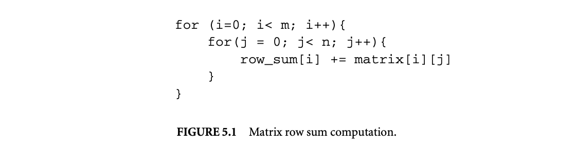 Normalized iteration number:: If a loop index I has a lower bound of L and a step size of S, then the normalized iteration number of an iteration is given by .
Iteration vector:: An iteration vector of a loop nest is a vector of integers representing loop iterations in which the value of the th component denotes the normalized iteration number of the th outermost loop. As an example, for the loop shown above, the iteration vector i = (1, 2) denotes the second iteration of the j loop within the first iteration of the i loop.
Using iteration vectors, we can define statement instances. A statement instance S(i) denotes the statement S executed on the iteration specified by the iteration vector i. Defining the dependence relations on statement instances, rather than just on the statements, makes the dependence definitions precise. Thus, if S denotes the statement row_sum[i] += matrix[i][j], then there is true dependence between and , where . In general, there can be a dependence between two statement instances and only if the statement is dependent on and the iteration vector is lexicographically less than or equal to . To specify dependence between statement instances, we define two vectors:
Dependence distance vector:: If there is a dependence from statement in iteration to statement in iteration , then the dependence distance vector is a vector of integers defined as -.
Dependence direction vector:: If is a dependence distance vector, then the corresponding direction vector is defined as
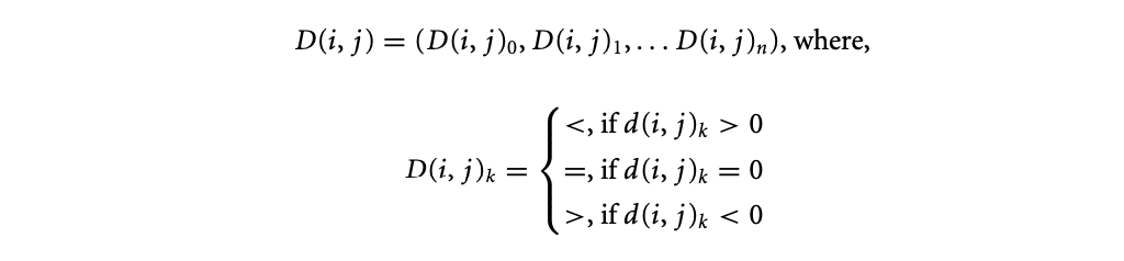
In any valid dependence, the leftmost non = component of the direction vector must be . The loop transformations described in this chapter are known as reordering transformations. A reordering transformation is one that does not add or remove statements from a loop nest and only reorders the execution of the statements that are already in the loop. Since reordering transformations do not add or remove statements, they do not add or remove any new dependences. A reordering transformation is valid if it preserves all existing dependences in the loop.
5.2.2 Reuse and Locality
Most compiler optimizations for memory hierarchies rely on the fact that programs reuse the same data repeatedly. There are two types of data reuse:
Temporal reuse:: When a program accesses a memory location more than once, it exhibits temporal reuse. Spatial reuse:: When a program accesses multiple memory locations within the same cache line, it exhibits spatial reuse.
These reuses can be due to the same reference or a group of data references. In the former case, the reuse is known as self reuse, and in the latter case, it is known as group reuse. In the loop
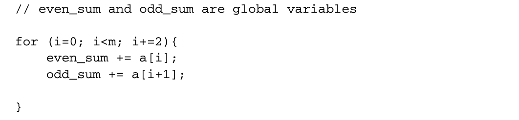 even_sum and odd_sum exhibit self-temporal reuse. The references to a[i] and a[i+1] show self-spatial reuse individually and exhibit group-spatial reuse together.
Data reuse is beneficial since a reused data item is likely to be found in the caches and hence incur a low average access latency. If the caches are infinitely large, then all reused data would be found in the cache, but since the cache sizes are finite, a data object D in the cache may be replaced by some other data between two uses of D.
5.2.3 Quantifying Reuse and Locality
The compiler must be able to quantify reuse and locality in order to exploit them. Reuse resulting from array accesses in loops whose subscripts are affine functions of the loop indices can be modeled using linear algebra. Consider an -dimensional array X accessed inside a loop nest loops. Let the loop indices be represented by an matrix . Then each access to X can be represented as X[], where is an matrix that applies a linear transformation on , and is an constant vector. For example, an access X[0][i-j] in a loop nest with two loops, whose indices are and , is represented as X[], where
 This access exhibits self-temporal reuse if it accesses the same memory location in two iterations of the loop. If, in iterations and , the reference to X accesses the same location, then must be equal to . Let . The vector is known as the reuse distance vector. If a non-null value of satisfyies the equation , then the reference exhibits self-temporal reuse. In other words, if the kernel of the vector space given by is non-null, then the reference exhibits self-temporal reuse. For the above example, there is a non-null satisfying the equation since . This implies that the location accessed in iteration is also accessed in iteration for any value of . Group-temporal reuse is identified in a similar manner. If two references and to the same array in iterations and , respectively, access the same location, then must be equal to . In other words, if a non-null satisfies , the pair of references exhibit group-temporal reuse. If an entry of the vector is 0, then the corresponding loop carries temporal reuse. The amount of reuse is given by the product of the iteration count of those loops that have a 0 entry in .
An access exhibits self-spatial reuse if two references access different locations that are in the same cache line. We define the term contiguous dimension to mean the dimension of the array along which two adjacent elements of the array are in adjacent locations in memory. In this chapter, all the code examples are in C, where arrays are arranged in row-major order and hence the th dimension of an -dimensional array is the contiguous dimension. For simplicity, it is assumed that two references exhibit self-spatial reuse only if they have the same subscripts in all dimensions except the contiguous dimension. This means the first test for spatial reuse is similar to that of temporal reuse ignoring the contiguous dimension subscript. The second test is to ensure that the subscripts of the last contiguous dimension differ by a value that is less than the cache line size. Given an access , the entries of the last row of matrix are coefficients of the affine function used as a subscript in the contiguous dimension. We define a new matrix that is obtained by setting all the columns in the last row of to 0. If the kernel of is non-null and the subscripts of the contiguous dimension differ by a value less than the cache line size, then the reference exhibits self-spatial reuse. Similarly, group-spatial reuse is present between two references and if there is a solution to . Let denote the iteration counts of loops that carry temporal reuse in all but the contiguous dimension. Let be the stride along the contiguous dimension and be the cache line size. Then, the total spatial reuse is given by .
As described earlier, reuse does not always translate to locality. The term data footprint of a loop invocation refers to the total amount of data accessed by an invocation of the loop. It is difficult to exactly determine the size of data accessed by a set of loops, so it is estimated based on factors such as estimatediteration count. The term localized iteration space[21] refers to the subspace of the iteration space whose data footprint is smaller than the cache size. Reuse translates into locality only if the intersection of the reuse distance vector space with the localized iteration vector space is not empty.
5.3 Loop Interchange
Loop interchange changes the order of loops in a perfect loop nest to improve spatial locality. Consider the loop in Figure 5.2. This loop adds two matrices. Since multidimensional arrays in C are stored in row-major order, two consecutive accesses to the same array are spaced far apart in memory. If all the three matrices do not completely fit within the cache, every access to a, b, and c will miss in the cache, but a compiler can transform the loop into the following equivalent loop:
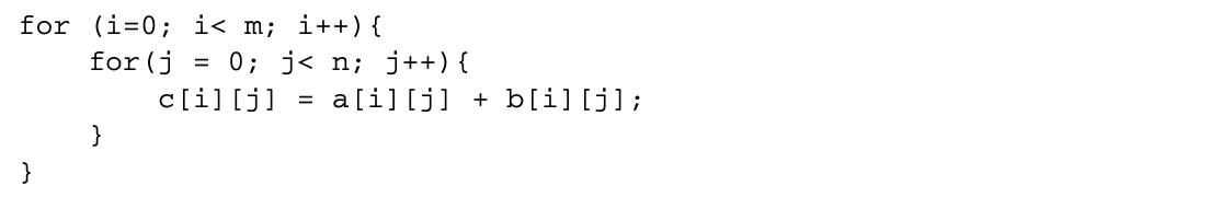 The above loop is semantically equivalent to the first loop but results in fewer conflict misses.
As this example illustrates, the order of nesting may be unimportant for correctness and yet may have a significant impact on the performance. The goal of loop interchange is to find a suitable nesting order that reduces memory access latency while retaining the semantics of the original loop. Loop interchange comes under a category of optimizations known as unimodular transformations. A loop transformation is called unimodular if it transforms the dependences in a loop by multiplying it with a matrix, whose determinant has a value of either or . Other unimodular transformations include loop reversal, skewing, and so on.
5.3.1 Legality of Loop Interchange
It is legal to apply loop interchange on a loop nest if and only if all dependences in the original loop are preserved after the interchange. Whether an interchange preserves dependence can be determined by looking at the direction vectors of the dependences after interchange. Consider a loop nest . Let be the direction vector of a dependence in this loop nest. If the order of loops in the loop nest is permuted by some transformation, then the direction vector corresponding to the dependence in the permuted loop nest can be obtained by permuting the entries of . To understand this, consider the iteration vectors and corresponding to the source and sink of the dependence. A permutation of the loop nest results in a corresponding permutation of the components of and . This permutes the distance vector and hence the direction vector . To determine whether can be permuted to , the same permutation is applied to the direction vectors of all dependences, and the resultant direction vectors are checked for validity.
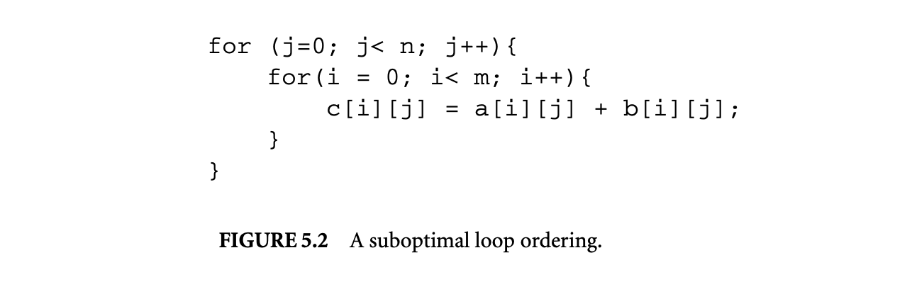 As an example, consider the loop
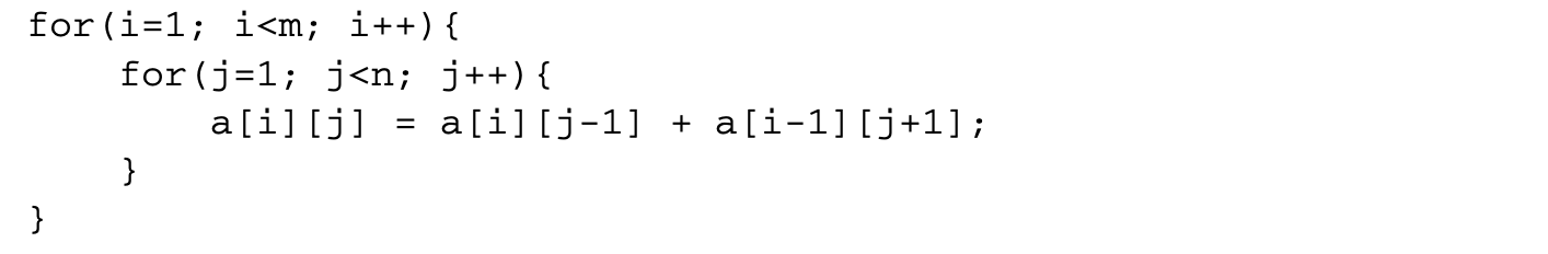 This loop nest has two dependences:
- Dependence from to , represented by the distance vector and the direction vector
- Dependence from to , represented by the distance vector and the direction vector
Loop interchange would permute a direction vector by swapping its two components. While the direction vector remains valid after this permutation, the vector gets transformed to , which is an invalid direction vector. Hence, the loop nest above cannot be interchanged.
5.3.2 Dependent Loop Indices
Even if interchange does not violate any dependence, merely swapping the loops may not be possible if the loop indices are dependent on one another. For example, the loop in Figure 5.1 can be rewritten as
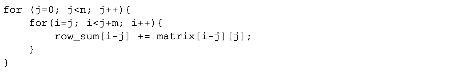 Except for the change in the bounds of the inner loop index, the loop is semantically identical to the one in Figure 5.1. It has the same dependence vectors, so it must be legal to interchange the loops. However, since the inner loop index is dependent on the outer loop index, the two loops cannot simply be swapped. The indices of the loops need to be adjusted after interchange. This can be done by noting that loop interchange transposes the iteration space of the loop. Figure 5.3 shows the iterations of the original loop for and . In Figure 5.4, the iteration space is transposed. This corresponds to the following interchanged loop.
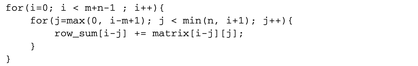
5.3.3 Profitability of Loop Interchange
Even if loop interchange can be performed on a loop nest, it is not always profitable to do so. In the example shown in Figure 5.2, it is obvious that traversing the matrices first along the rows and then along the columns is optimal, but when the loop body accesses multiple arrays, each of the accesses may prefer a different loop order. For example, in the following loop
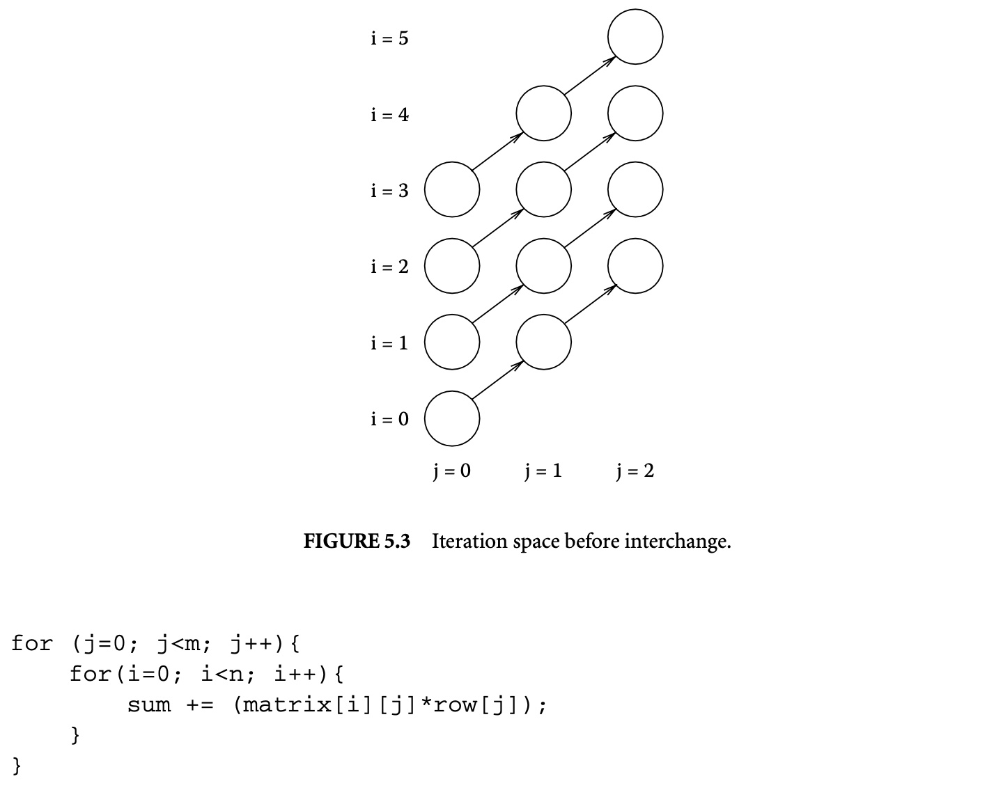
the loop order is suboptimal for accesses to the matrix array. However, this is the best loop order to access the row array. In this loop nest, the element row[j] shows self-temporal reuse between the iterations of the inner loop. Hence, it needs to be accessed just once per iteration of the outer loop. If the loops are interchanged, this array is accessed once per iteration of the inner loop. If the size of the row array is much larger than the size of the cache, then there is no reuse across outer loop iterations.
For this loop nest:
- Number of misses to matrix =
- Number of misses to row =
- Total number of misses =
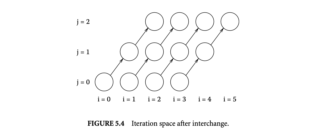
If the loops are interchanged, then
- Number of misses to
- Number of misses to
- Total number of misses
In the above equations, cls denotes the size of the cache line in terms of elements of the two arrays. From this set of equations, it is clear that the interchanged loop is better only when the cache line can hold more than two elements of the two arrays.
5.3.4 A Loop Permutation Algorithm
In theory, one could similarly determine the right order for any given loop nest, but when the maximum depth of a perfect loop nest is , the number of possible loop orderings is , and computing the total number of misses for those loops is prohibitive for a large value of . Instead, we can use some simple set of heuristics to determine an order that is likely to be profitable.
The algorithm in Figure 5.5 computes a good order of loops for the given loop nest . For every loop in , it computes cache_misses(L), which is the estimated number of cache misses when the loop L is made the inner loop. To compute cache_misses(L), the algorithm first computes a set. Each element of this set is either a single array reference or a group of array references that have group reuse. For instance, in the following loop,
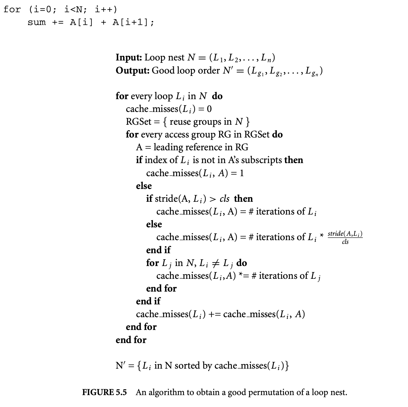
array references and belong to the same reuse group. Only the leading array reference in a reuse group is used for calculating cache_misses. If a reference does not have in the subscripts, its cost is considered as 1. This is because such a reference will correspond to the same memory location for all iterations of and will therefore miss only once during the first access. If a reference has the index of in one of its subscripts, the stride of the reference is first computed. is defined as the difference in address in accesses of A in two consecutive iterations of , where the th component of the iteration vector differs by 1. As an example, is 256 in the following code:
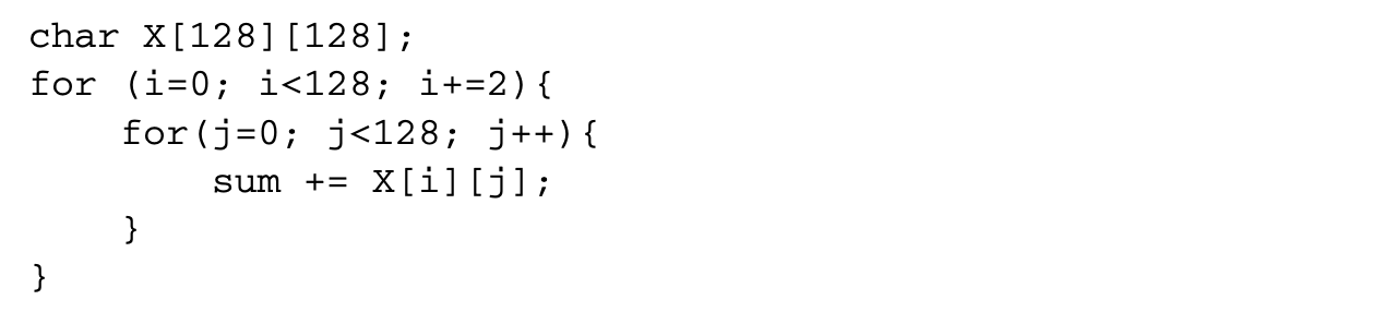
If the stride is greater than the cache line size, then every reference to A will miss in the cache, so cache_misses is incremented by the number of iterations of . If the stride is less than cache line size, then only one in every accesses will miss in the cache. Hence, the number of iterations of is divided by and added to cache_misses(). Then, for each reference, cache_misses() is multiplied by the iteration counts of other loops whose indices are used as some subscript of A. Finally, the cache_misses for all references are added together.
After cache_misses() for each loop is computed, the loops are sorted by cache_misses in descending order, and this is to obtain a good loop order. In other words, the loop with the lowest estimated cache misses is a good candidate for the innermost loop, the loop with the next lowest cache misses is a good candidate for the next innermost loop, and so on.
To see how this algorithm works, it is applied to the loop
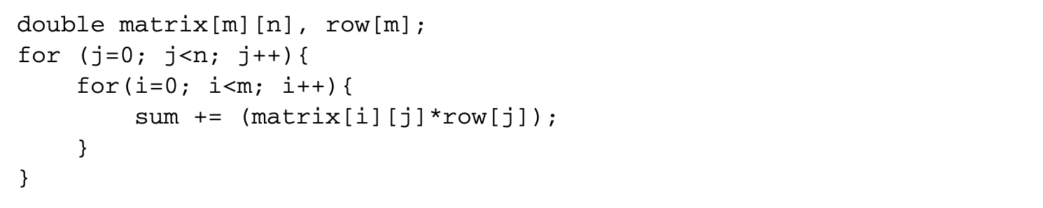 Let denote the loop with induction variable i and denote the loop with induction variable j. For the loop nest with i as the induction variable:
- cache_misses(, row) = , since is not a subscript in row.
- cache_misses(, matrix) = . Here we assume that is a large enough number so that stride(, ) is greater than the cache line size.
- cache_misses() = .
For the loop :
- cache_misses(, row) = sizeof(double)/cls
- cache_misses(, matrix) = sizeof(double)/cls
- cache_misses() = sizeof(double)/cls
If the cache line can hold at least two doubles, cache_misses() is less than cache_misses(), and therefore is the candidate for the inner loop position.
While the algorithm in Figure 5 determines a good loop order in terms of profitability, it is not necessarily a valid order, as some of the original dependences may be violated in the new order. The order produced by the algorithm is therefore used as a guide to obtain a good legal order. This can be done in the following manner:
- Pick the best candidate for the outermost loop among the loops that are not yet in the best legal order.
- Assign it to the outermost legal position in the best legal order.
- Repeat steps 1 and 2 until all loops are assigned a place in the best legal order.
Kennedy and Allen [13] show why the resulting order is always a legal order.
5.4 Loop Blocking
A very common operation in many scientific computations is matrix multiplication. The code shown below is a simple implementation of the basic matrix multiplication algorithm.
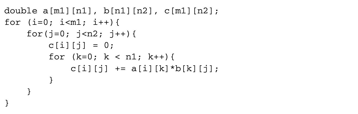 This code has a lot of data reuse. For instance, every row of matrix a is used to compute n2 different elements of the product matrix c. However, this reuse does not translate to locality if the matrices do not fit in the cache. If the matrices do not fit in the cache, the loop also suffers from capacity misses that are not eliminated by loop interchange. In this case, the following transformed loop improves locality:
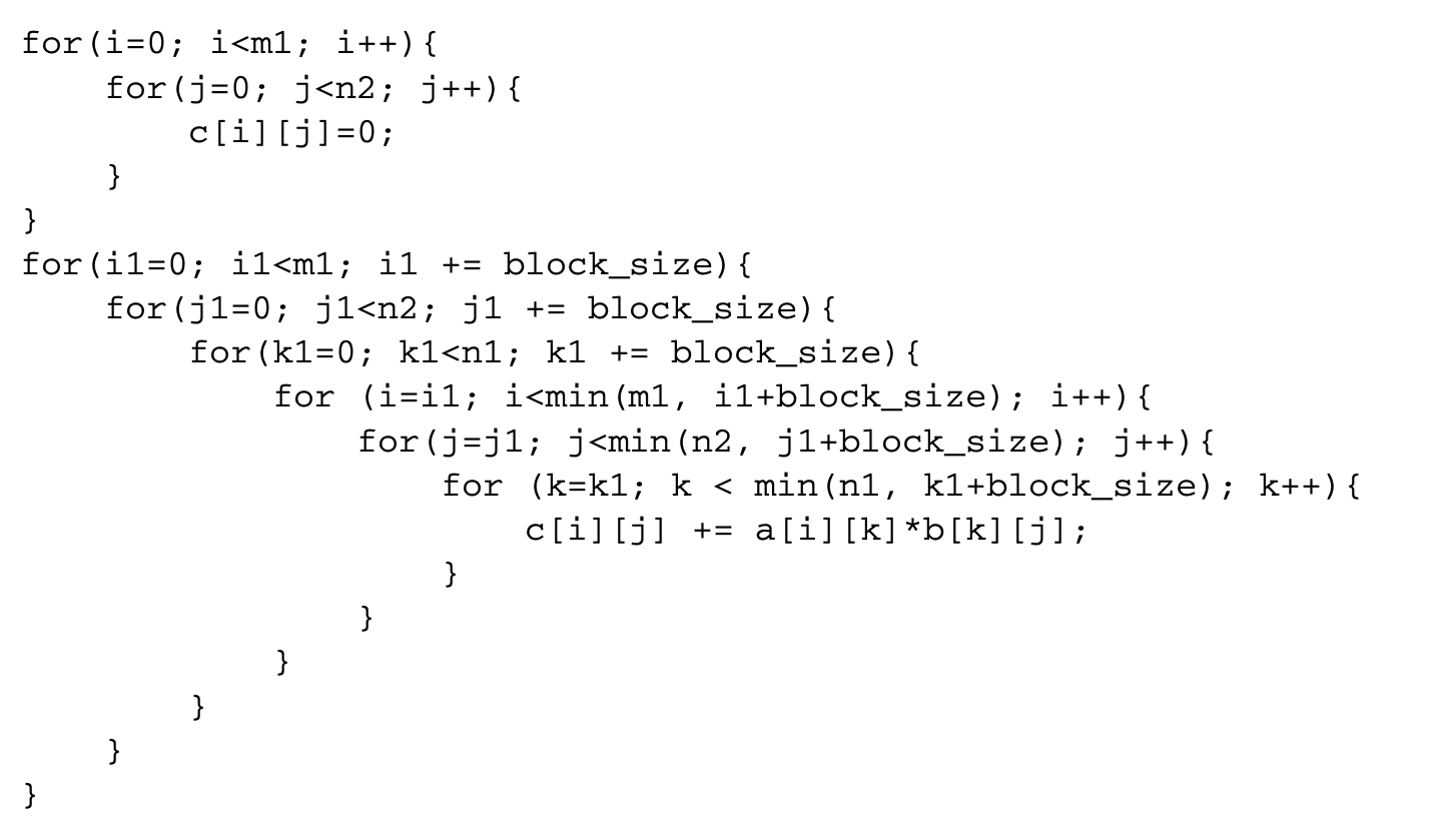
First the initialization of the matrix c is separated out from the rest of the loop. Then, a transformation known as blocking or tiling is applied. If the value of block_size is chosen carefully, the reuse in the innermost three loops translates to locality. Figures 5.6 and 5.7 show the iteration space of a two-dimensional loop nest before and after blocking. In this example, the original iteration space has been covered by using four nonoverlapping rectangular tiles or blocks. In general, the tiles can take the shape of a parallelepiped for an -dimensional iteration space. A detailed discussion of tiling shapes can be found in Rajopadhye [24].
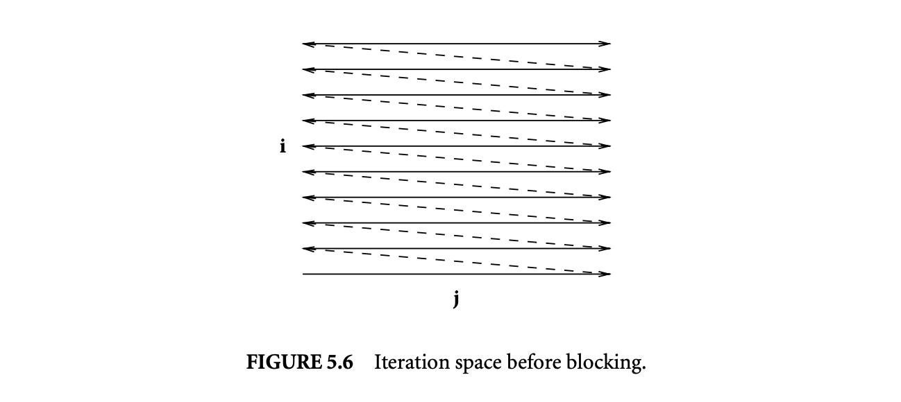 The basic transformation used in blocking is called strip-mine and interchange. Strip mining transforms a loop into two nested loops, with the inner loop iterating over a small strip of the original loop and the outer loop iterating across strips. Strip mining the innermost loop in the matrix multiplication example results in the following loop nest:
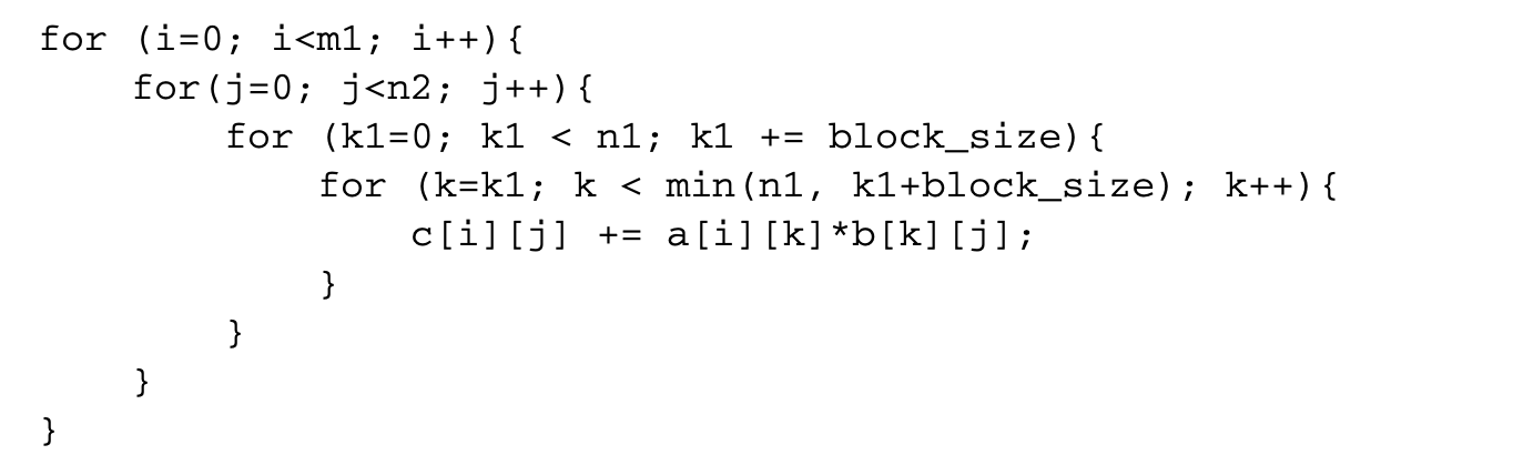 Assuming block_size is smaller than n1, the innermost loop now executes fewer iterations than before, and there is a new loop with index k1. After strip mining, the loop with index k1 is interchanged with the two outer loops, resulting in blocking along one dimension:
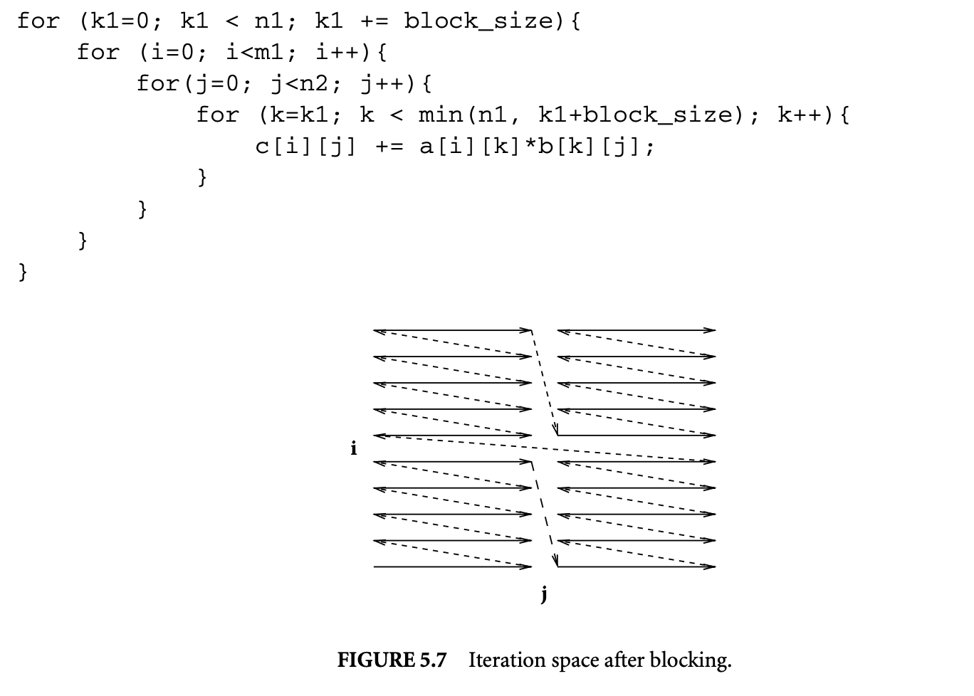 Doing strip-mine and interchange on the and loops also results in the blocked matrix multiplication code shown earlier. An alternative approach to understand blocking in terms of clustering and tiling matrices is discussed by Rajopadhye [24].
5.4.1 Legality of Strip-Mine and Interchange
Let be a loop which is to be strip mined into an outer loop and an inner loop . Let be the loop with which the loop is to be interchanged. Strip mining is always a legal transformation since it does not alter any of the existing dependences and only relabels the iteration space of the loop. Thus, the legality of blocking depends on the legality of the interchange of and , but determining the legality of this interchange requires strip mining , which necessitates the recomputation of the direction vectors of all the dependences. A faster alternative is to test the legality of interchanging with instead. While the legality of this interchange ensures the correctness of blocking, this test is conservative and may prevent valid strip-mine and interchange in some cases 1.
5.4.2 Profitability of Strip-Mine and Interchange
We now discuss the conditions under which strip-mine and interchange transformation is profitable, given the strip sizes, which determine the block size. For a discussion of optimal block sizes refer to Rajopadhye [24] (Chapter 15 in this text).
Given a loop nest , a loop and another loop , where is nested within , the profitability of strip mining and interchanging the by-strip loop with depends on the following:
- The reuse carried by
- The data footprint of all inner loops of
- The cost of strip mining
The goal of strip mining and interchanging the by-strip loop with is to ensure that reuse carried by is translated into locality. For this to happen, must carry reuse between its iterations. This can happen under any of the following circumstances:
- There is some dependence carried by . If carries some dependence, it means an iteration of reuses a location accessed by some earlier iteration of .
- There is an array index that does not have the index of in any of its subscripts.
- The index of is used as a subscript in the contiguous dimension, resulting in spatial reuse.
The data footprint of must be larger than the cache size, as otherwise the reuse carried by lies within the localized iteration space. The data footprint of must also be larger than the cache size, as otherwise it is sufficient to strip-mine some other loop between and . Finally, the benefits of reuse must still outweigh the cost of strip mining . Strip mining can cause a performance penalty in two ways:
- If the strips are not aligned to cache line boundaries, it would reduce the spatial locality of array accesses that have the index of as the subscript in the contiguous dimension.
- Every dependence carried by the loop shows decreased temporal locality.
Typically, the cost of doing strip-mine and interchange is small and is often outweighed by the benefits.
5.4.3 Blocking with Skewing
In loop nests where interchange violates dependences, loop skewing can be applied first to enable loop interchange. Consider the loop iteration shown in Figure 5.8. The outer loop of this nest is indexed by , and the inner loop by . Even if it is profitable, the diagonal edges from iteration vector to prevent loop interchange, but the same loop can be transformed to the one in Figure 5.9, which allows loop interchange. This transformation is known as loop skewing.
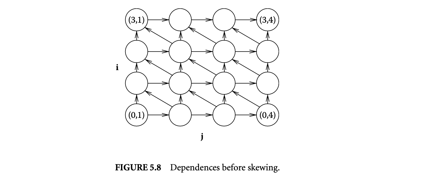 Given two loops, the inner loop can be skewed with respect to the outer loop by adding the outer loop index to the inner loop index. Consider a dependence with direction vector . This pair of loops does not permit loop interchange. Consider two iteration vectors and , which are the source and target, respectively, of the dependence. Let be the distance vector corresponding to this dependence, where . The goal is to transform this distance vector into , where , so that the direction vector becomes either or , which permits loop interchange. This can be achieved by multiplying the outer loop index and adding the product to the inner loop index. Thus, the two iteration vectors become and , and the distance vector becomes , which is equal to .
The loop shown in Figure 5.8 applies an averaging filter times on an array as shown below:
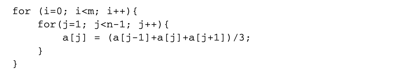 The dependences in this loop are characterized by three dependence distance vectors , and , which are depicted in Figure 5.8, for the case where takes a value of 4 and takes a value of 6. While the loop can be strip mined into two loops with induction variables and , the loop cannot be interchanged with the loop because of the dependence represented by . We skew the inner loop with respect to the outer loop.
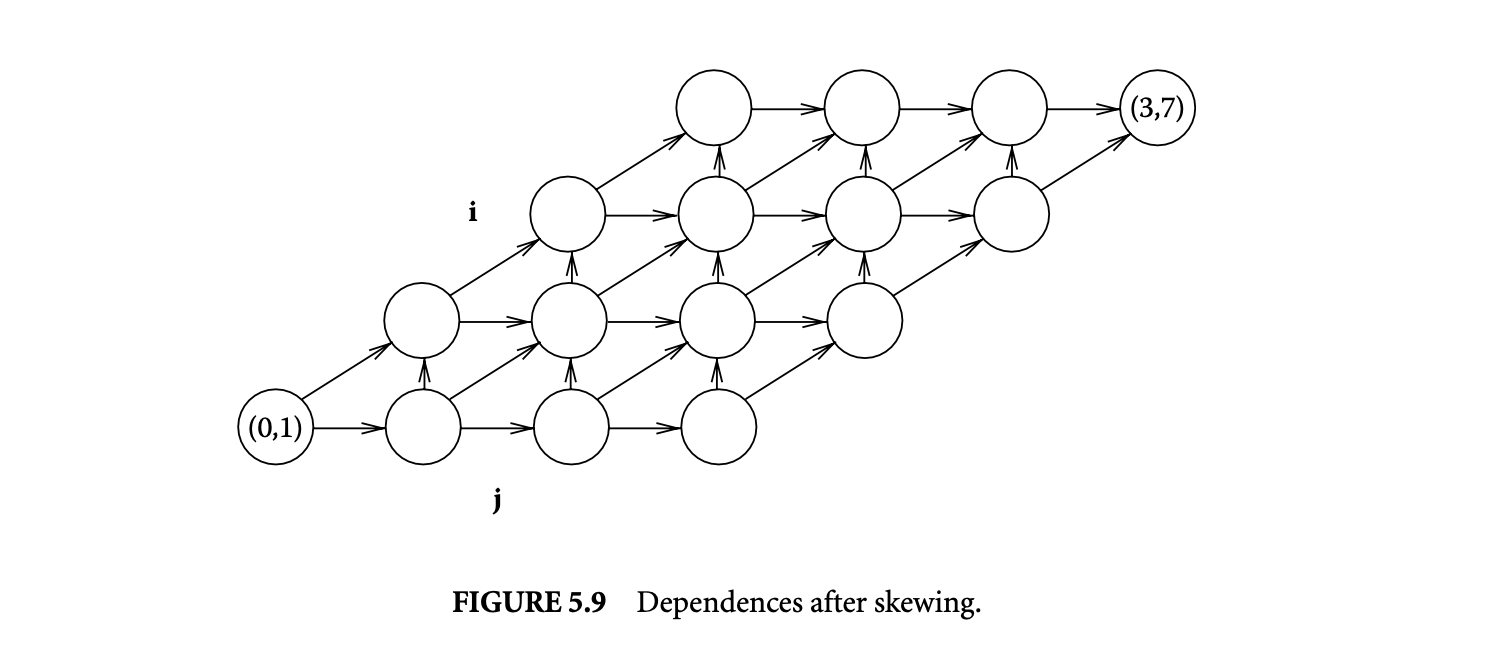
Since a distance vector of allows interchange, the value of is chosen as 1. Figure 5.9 shows the dependences in the loop after applying skewing. This corresponds to the following loop:
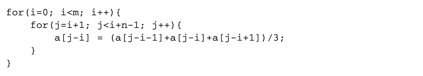 Strip mining the loop with index j results in the following code:
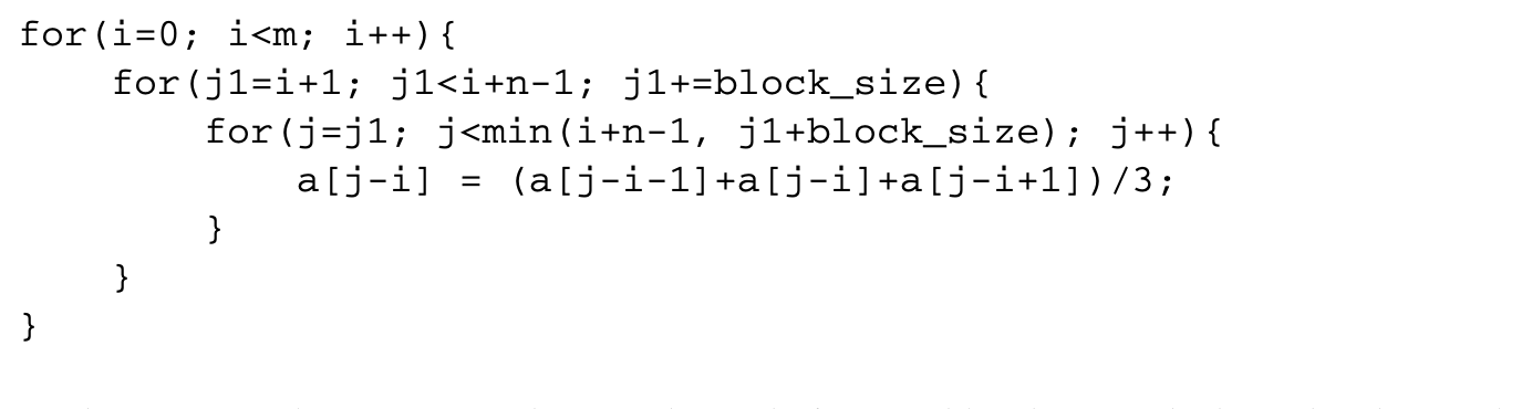 The outer two loops can now be interchanged after suitably adjusting the bounds. This results in the tiled loop:
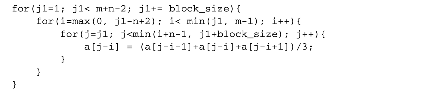
5.5 Other Loop Transformations
5.5.1 Loop Fusion
When there is reuse of data across two independent loops, the loops can be fused together, provided their indices are compatible. For example, the following set of loops:
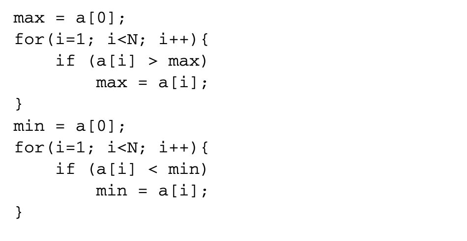 can be fused together into a single loop:
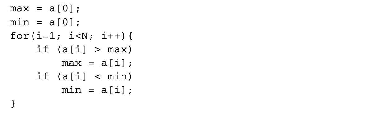
If the value of N is large enough that the array does not fit in the cache, the original loop suffers from conflict misses that are minimized by the fused loop. Loop fusion is often combined with loop alignment. Two loops may have compatible loop indices, but the bounds may be different. For example, if the first loop computes the maximum of all elements and the second loop computes the minimum of only the first elements, the indices have to be aligned. This is done by first splitting the max loop into two, one iterating over the first elements and the other over the rest of the elements. Then the loop computing the minimum can be fused with the first portion of the loop computing the maximum.
5.5.2 Loop Fission
Loop fission or loop distribution is a transformation that does the opposite of loop fusion by transforming a loop into multiple loops such that the the body of the original loop is distributed across those loops. To determine whether the body can be distributed, the program dependence graph (PDG) of the loop body is constructed first. Different strongly connected components of the PDG can be distributed into different loops, but all nodes in the same strongly connected component have to be in the same loop. For example, the following loop,
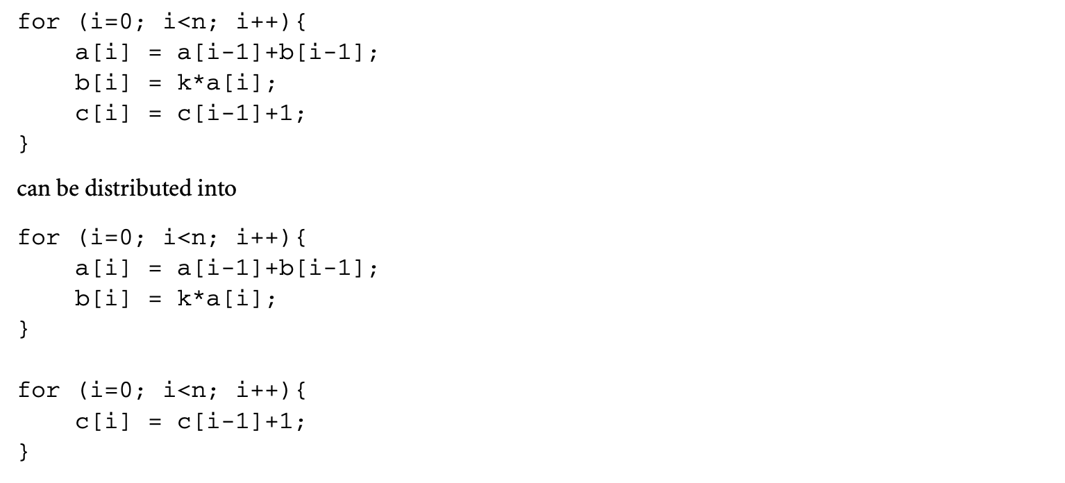 since the statement is independent of the other two statements, which are dependent on each other. Loop fission reduces the memory footprint of the original loop. This is likely to reduce the capacity misses in the original loop.
5.6 Data Prefetching
Data prefetching differs from the other loop optimizations discussed above in some significant aspects:
-
Instead of transforming the data access pattern of the original code, prefetching introduces additional code that attempts to bring in the cache lines that are likely to be accessed in the near future.
-
Data prefetching can reduce all three types of misses. Even when it is unable to avoid a miss, it can reduce the time to service that miss.
-
While the techniques described above are applicable only for arrays, data prefetching is a much more general technique.
-
Prefetching requires some form of hardware support.
Consider the simple loop
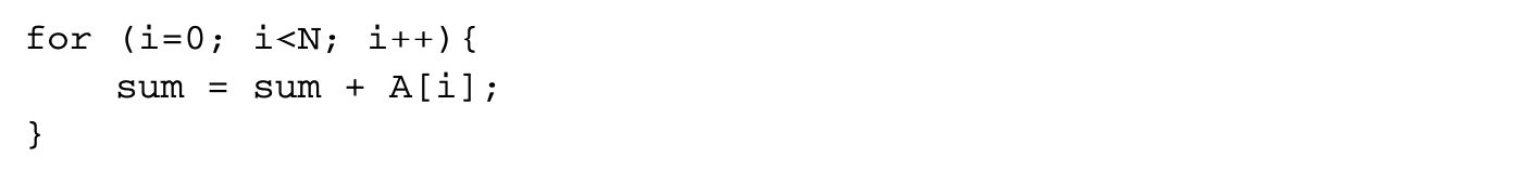
This loop computes the sum of the elements of the array A. The cache misses to the array A are all cold misses. To avoid these misses, prefetching code is inserted in the loop to bring into the cache an element that is required some pd iterations later:
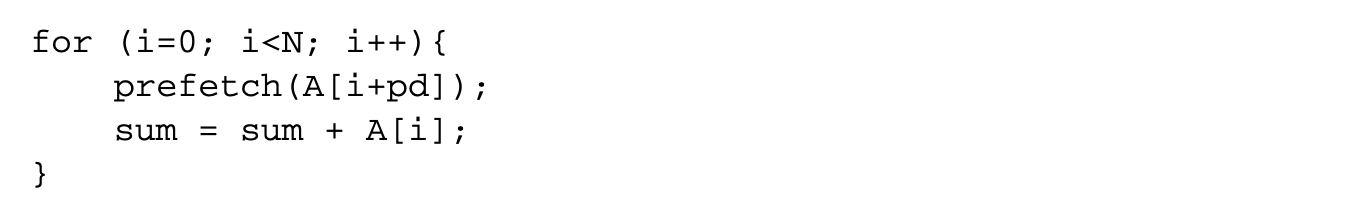 The value above is referred to as the prefetch distance, which specifies the number of iterations between the prefetching of a data element and its actual access. If the value of is carefully chosen, then on most iterations of the loop, the array element that is accessed in that iteration would already be available in the cache, thereby minimizing cold and capacity misses.
5.6.1 Hardware Support
In the above example, we have shown prefetch as a function routine. In practice, prefetch corresponds to some machine instruction. The simplest option is to use the load instruction to do the prefetch. By loading the value to some unused register or a register hardwired to a particular value and making sure the instruction is not removed by dead code elimination, the array element is brought into the cache. While this has the advantage of requiring no additional support in the instruction set architecture (ISA), this approach has some major limitations. First, the load instructions have to be nonblocking. A load instruction is nonblocking if the load miss does not stall other instructions in the pipeline that are independent of the load. If the load blocks the pipeline, the prefetches themselves would suffer cache misses and block the pipeline, defeating the very purpose of prefetching. This is not an issue in most modern general-purpose processors, where load instructions are nonblocking. The second, and major, limitation is that since executing loads can cause exceptions, prefetches might introduce new exceptions in the transformed code that were not there in the original code. For instance, the code example shown earlier might cause an exception when it tries to access an array element beyond the length of the array. This can be avoided by making sure an address is prefetched only if it is guaranteed not to cause an exception, but this would severely limit the applicability of prefetching. To avoid such issues, some processors have special prefetch instructions in their instruction set architecture. These instructions do not block the pipeline and silently ignore any exceptions that are raised during their execution. Moreover, they typically do not use any destination register, thereby improving the register usage in code regions with high register pressure.
5.6.2 Profitability of Prefetching
Introducing data prefetching does not affect the correctness of a program, except for the possibility of spurious exceptions discussed above. When there is suitable ISA support to prevent such exceptions, the compiler has to consider only the profitability aspect when inserting prefetches. For a prefetch instruction to be profitable, it has to satisfy two important criteria: accuracy and timeliness.
Accuracy refers to the fact that a prefetched cache line is actually accessed later by the program. Prefetches may be inaccurate because of the compiler's inability to determine runtime control flow. Consider the following loop:
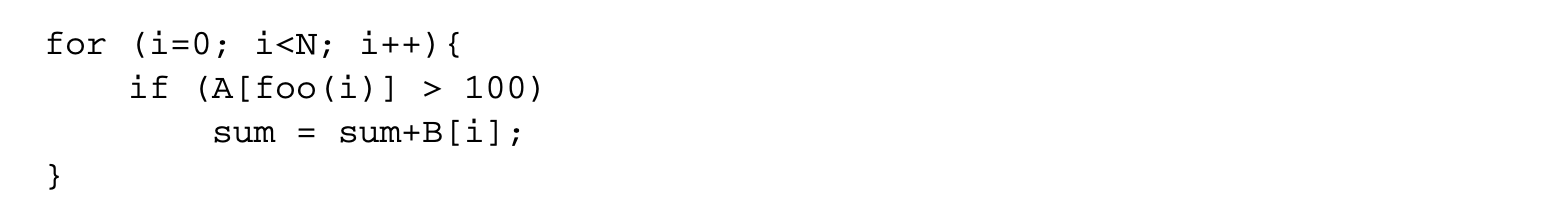 A prefetch for the array B inserted at iteration is accurate only if the element B[i+pd] is accessed later, but this depends on A[foo(i+pd)], and it may not always be safe to compute foo(i+pd). Even if it is safe to do so, the cost of invoking foo may far outweigh the potential benefits of prefetching, forcing the compiler to insert prefetches unconditionally for every future iteration. As will be described later, prefetching of a loop traversing a recursive data structure could also be inaccurate. The accuracy of a prefetch is important because useless prefetches might evict useful data -- data that will definitely be accessed in the future -- from the cache line and increase the memory traffic, thereby degrading the performance.
Accuracy alone does not guarantee that a prefetch is beneficial. If we set the value of to be 0, then we can guarantee that the prefetch is accurate by issuing it right before the access, but this obviously does not result in any benefit. A prefetch is timely if it is issued at the right time, so that, when the access happens, it finds the data in the cache. The prefetch distance determines the timeliness of a prefetch for a given loop. Let be the average schedule height of a loop iteration and be the prefetch distance. Then the number of cycles separating the prefetch and the actual access is roughly . This value must be greater than the access latency without prefetch for the access to be a hit in the L1 cache. At the same time, if this value is too high, the probability of the prefetched cache line being displaced subsequently, before the actual access, increases, thereby reducing the benefits of the prefetch. Thus, determining the right prefetch distance for a given loop is a crucial step in prefetching implementations.
A third factor that determines the benefits of prefetching is the overhead involved in prefetching. The following example shows how the prefetching overhead could negate the benefits of prefetching. Consider the code fragment
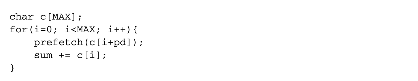 This code is the same as the example shown earlier, except that it sums up an array of chars. Assume that this code is executed on a machine with an issue width of 1, and the size of the L1 cache line is 64 bytes. Let be the number of cycles required to service a cache miss. Under this scenario,
 Even if all the misses are prefetched,

For prefetching to be beneficial,

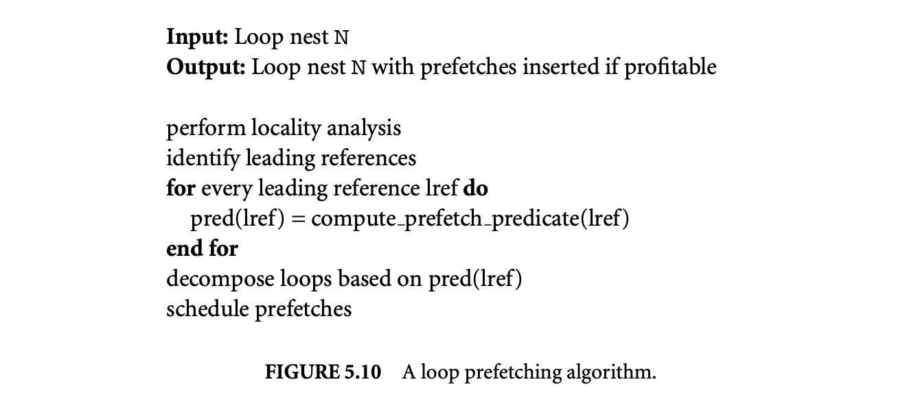
If the miss latency for this access without prefetching is 64 cycles, then the overhead of prefetching outweighs its benefits. In such cases, optimizations such as loop splitting or loop unrolling can make prefetching still be profitable. If the value of is determined, either statically or using profiling, to be a large number, unrolling the loop 64 times will make prefetching profitable. After unrolling, only one prefetch is issued per iteration of the unrolled loop, and hence the prefetching overhead reduces to cycles. For prefetching to be beneficial in this unrolled loop,
 Thus, as long as the cost of a cache miss is more than one cycle, prefetching will be beneficial.
5.6.3 Prefetching Affine Array Accesses
Figure 5.10 outlines an algorithm by Mowry et al. [21] that issues prefetches for array accesses within a loop.
The prefetching algorithm consists of the following steps:
-
Perform locality analysis. The first step of the algorithm is to obtain reuse distance vectors and intersect them with the localized iteration space to determine the locality exhibited by the accesses in the loop.
-
Identify accesses requiring prefetches. All accesses exhibiting self-reuse are candidates for prefetching. When accesses exhibit group reuse, only one of the accesses needs to be prefetched. Among references that exhibit group reuse, the one that is executed first is called the leading reference. It is sufficient to prefetch only the leading reference of each group.
-
Compute prefetch predicates. When a reference has spatial locality, multiple instances of that reference access the same cache line, so only one of them needs to be prefetched. To identify this, every instance of an access is associated with a prefetch predicate. An instance of a reference is prefetched only if the predicate associated with it is 1. Since all references are affine array accesses, the predicates are some functions of the loop indices. As an example, consider the following loop nest:
 Assuming that the arrays are aligned to cache line boundaries, the prefetch predicate for sum is and for a is , where n is the number of elements of a in a cache line.
 -
Perform loop decomposition. One way to ensure that a prefetch is inserted only when the predicate is true is to use a conditional statement based on the prefetch predicate or, if the architecture supports it, use predicate registers to guard the execution of the prefetch. This requires computing the predicate during every iteration of the loop, which takes some cycles, and issuing the prefetch on every iteration, which takes up issue slots. Since the prefetch predicates are well-defined functions of the loop indices, a better approach is to decompose the loop into sections such that all iterations in a particular section either satisfy the predicate or do not satisfy the predicate. The code above, with respect to the reference to array a, satisfies the predicate in iterations 0, n, 2n, and so on and does not satisfy the predicates in the rest of the iterations. There are many ways to decompose the loops into such sections. If a prefetch is required only during the first iteration of a loop, then the first iteration can be peeled out of the loop and the prefetch inserted only in the peeled portion. If the prefetch is required once in every iterations, the loop can be unrolled times so that in the unrolled iteration space, every iteration satisfies the predicate. However, depending on the unroll factor and the size of the loop body, unrolling might degrade the instruction cache behavior. In those cases, the original iterations that do not satisfy the prefetching predicate can be rerolled back. For instance, if the loop above is transformed into all iterations of the inner loop do not satisfy the predicate, while all iterations of the outer loop satisfy the predicate. This process is known as loop splitting. This is performed for all distinct prefetch predicates.
-
Schedule the prefetches. A prefetch has to be timely to be effective. If cyclesmiss denotes the cache miss penalty in terms of cycles, then the prefetch has to be inserted that many cycles before the reference to completely eliminate the miss penalty. This can be achieved by software pipelining the loop, assuming that the latency of the prefetch instruction is cyclesmiss. This will have the effect of moving the prefetch instruction iterations ahead of the corresponding access in the software pipelined loop.
Certain architecture-specific features can also be used to enhance the last two steps above. For example, the Intel Itanium(r) architecture has a feature known as rotating registers. This allows registers used in a loop body to be efficiently renamed after every iteration of a counted loop such that the same register name used in the code refers to two different physical registers in two consecutive iterations of the loop. The use of rotating registers to produce better prefetching code is discussed in [8].
5.6.4 Prefetching Other Accesses
Programs often contain other references that are predictable. These include:
- Arrays with subscripts that are not affine functions of the loop indices but still show some predictability of memory accesses
- Traversal of a recursive data structure such as a linked list, where all the nodes in the list are allocated together and hence are placed contiguously
- Traversal of a recursive data structure allocated using a custom allocator that allocates objects of similar size or type together
A compiler cannot statically identify and prefetch such accesses and usually relies on some form of runtime profiling to analyze these accesses. A technique known as stride profiling[35] is often used to identify such patterns. The goal of stride profiling is to find whether the addresses produced by a static load/storeinstruction exhibit any exploitable pattern. Let denote the addresses generated by a static load/store instruction. Then denote the access strides. An instruction is said to be strongly single strided if most of the s are equal to some . In other words, there is some such that is close to 1. This profiled stride is used in computing the prefetch predicate and scheduling of the prefetch. Some instructions may not have a single dominant stride but still show regularity. For instance, a long sequence of may all be equal to , followed by a long sequence of being all equal to , and so on. In other words, an access has a particular stride in one phase, followed by a different stride in the next phase, and so on. Such accesses are called strongly multi-strided. The following example illustrates how a strongly multi-strided access can be prefetched:
 Ifptr is found to be strongly multi-strided, it can be prefetched as follows:
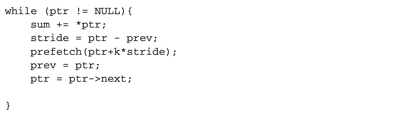 The loop contains code to dynamically calculate the stride. Assuming that phases with a particular stride last for a long time, the current observed stride is used to prefetch the pointer that is likely to be accessed iterations later. Since the overhead of this prefetching is high, it must be employed judiciously after considering factors such as the iteration count of the loop, the average access latency of the load that is prefetched, and the length of the phases with a single stride.
Another type of access that is useful to prefetch is indirect access. In the code fragment
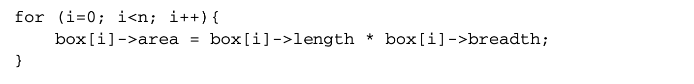 the references to the array box can be prefetched. However, the references to area, length, and breadth may cause a large number of cache misses if the pointers stored in the box array do not point to contiguous memory locations. Profile-based prefetching techniques are also not helpful in this case. The solution is to perform indirect prefetching. After applying indirect prefetching, the loop would look like
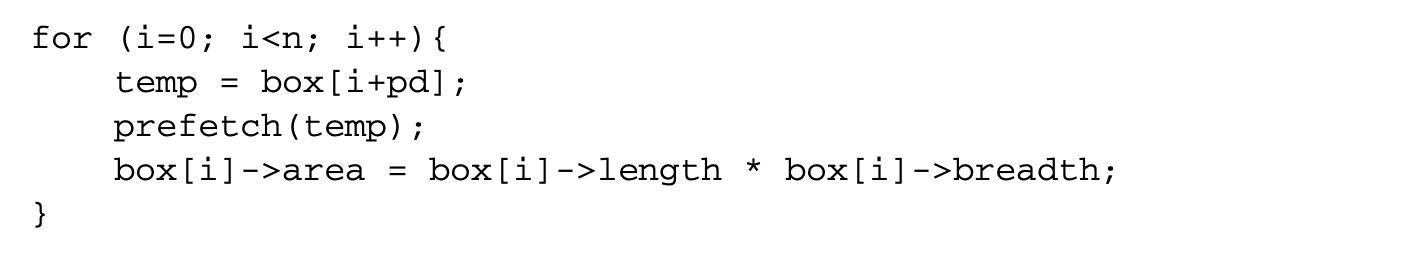 The pointer that would be dereferenced pd iterations later is loaded into a temporary variable, and a prefetch is issued for that address. The new loop requires a prefetch to box[i+pd], as otherwise the load to temp could result in stalls that may negate any benefits from indirect prefetching.
5.7 Data Layout Transformations
The techniques discussed so far transform the code accessing the data so as to decrease the memory access latency. An orthogonal approach to reduce memory access latency is to transform the layout of data in memory. For example, if two pieces of data are always accessed close to each other, the spatial locality can be improved by placing those two pieces of data in the same cache line. Data layout transformations are a class of optimization techniques that optimize the layout of data to improve spatial locality. These transformations can be done either within a single aggregate data type or across data objects.
5.7.1 Field Layout
The fields of a record type can be classified as hot or cold depending on their access counts. It is often beneficial to group hot fields together and separate them from cold fields to improve cache utilization. Consider the following record definition:
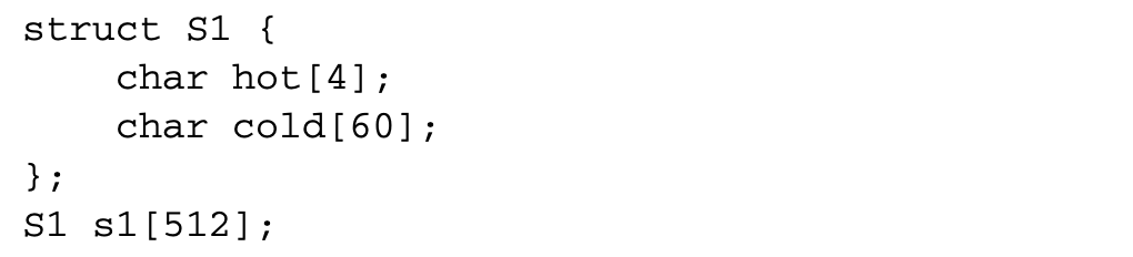 Each instance of S1 occupies a single cache line, and the entire array s1 occupies 512 cache lines. The total size of this array is well above the size of L1 cache in most processors, but only 4 bytes of the above record type are used frequently. If the struct consists of only the field hot, then the entire array fits within an L1 cache.
Structure splitting involves separating a set of fields in a record type into a new type and inserting a pointer to this new type in the original record type. Thus, the above struct can be transformed to:
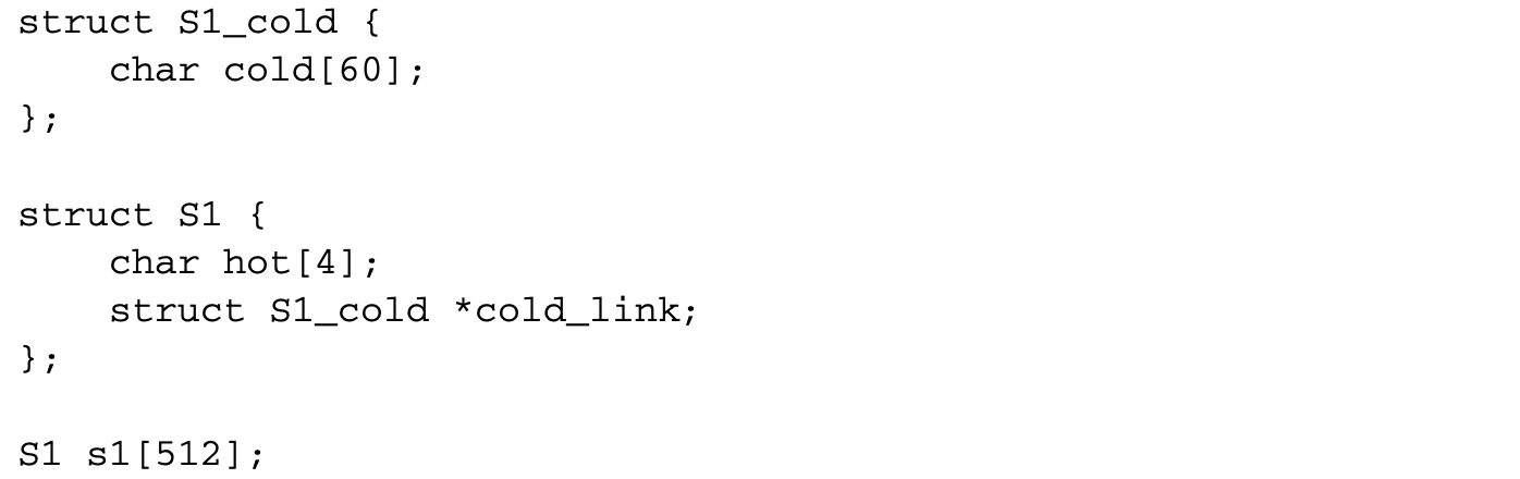 After the transformation, the array s1 fits in L1 cache of most processors. While this increases the cost of accessing cold, as it requires one more indirection, this does not hurt much because it is accessed infrequently. However, even this cost can be eliminated for the struct defined above, by transforming S1, as follows:
 The above transformation is referred to as structure peeling. While peeling is always better than splitting in terms of access costs, it is sometimes difficult to peel a record type. For instance, if a record type has pointers to itself, then peeling becomes difficult.
While merely grouping the hot fields together is often useful, this method suffers from performance penalties when the size of the record is large. As an example, consider the following record definition and some code fragments that use the record:
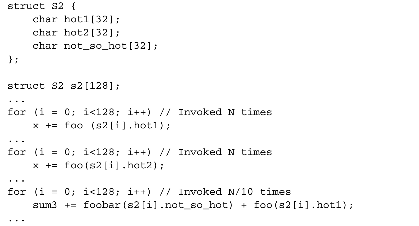 The fields hot1 and hot2 are more frequently accessed than not_so_hot, but not_so_hot is always accessed immediately before hot1. Hence placing not_so_hot together with hot1 improves spatial locality and reduces the misses to hot1. This fact is captured by the notion of reference affinity. Two fields have a high reference affinity if they are often accessed close to each other. In the above example, we have considered accesses within the same loop as affine. One could also consider other code granularities such as basic block, procedure, arbitrary loop nest, and so on.
Structure splitting, peeling, and re-layout involve the following steps:
The fields hot1 and hot2 are more frequently accessed than not_so_hot, but not_so_hot is always accessed immediately before hot1. Hence placing not_so_hot together with hot1 improves spatial locality and reduces the misses to hot1. This fact is captured by the notion of reference affinity. Two fields have a high reference affinity if they are often accessed close to each other. In the above example, we have considered accesses within the same loop as affine. One could also consider other code granularities such as basic block, procedure, arbitrary loop nest, and so on.
Structure splitting, peeling, and re-layout involve the following steps:
- Determine if it is safe to split a record type. Some examples of the unsafe behaviors include:
-
(a) Implicit assumptions on offset of fields. This typically involves taking the address of a field within the record.
-
(b) Pointers passed to external routines or library calls. This can be detected using pointer escape analysis.
-
(c) Casting from or to the record type under consideration. Casting from type A to type B implicitly assumes a particular relative ordering of the fields in both A and B. If a record type is subjected to any of the above, it is deemed unsafe to transform.
- Classify the fields of a record type as hot or cold. This involves computing the dynamic access counts of the structure fields. This can be done either using static heuristics or using profiling. Then fields whose access counts are above a certain threshold are labeled as hot and the other fields are labeled as cold.
- Move the cold fields to a separate record and insert a pointer to this cold record type in the original type.
- Determine an ordering of the hot fields based on the reference affinity between them. This involves the following steps:
- Compute reference affinity between all pairs of fields using some heuristic.
- Group together fields that have high affinity between them.
5.7.2 Data Object Layout
Data object layout attempts to improve the layout of data objects in stack, heap, or global data space. Some of the techniques for field layout are applicable to data object layout as well. For instance, the local variables in a function can be treated as fields of a record, and techniques for field layout can be applied. Similarly, all global variables can likewise be considered as fields of a single record type.
However, additional aspects of the data object layout problem add to its complexity. One such aspect is the issue of cache line conflicts. Two distinct cache lines containing two different data objects may conflict in the cache. If those two data objects are accessed together frequently, a large number of conflict misses may result. Conflicts are usually not an issue in field layout because the size of structures rarely exceeds the size of the cache, while global, stack, and heap data exceed the cache size more often.
Heap layout is usually more challenging because the objects are allocated dynamically. Placing a particular object at some predetermined position relative to some other object in the heap requires the cooperation of the memory allocator. Thus, all heap layout techniques focus on customized memory allocation that uses runtime profiles to guide allocation. The compiler has little role to play in most of these techniques.
A different approach to customized memory allocation, known as pool allocation, has been proposed by Lattner and Adve[14]. Pool allocation identifies the data structure instances used in the program. The allocator then tries to allocate each data structure instance in its own pool. Consider the following code example:
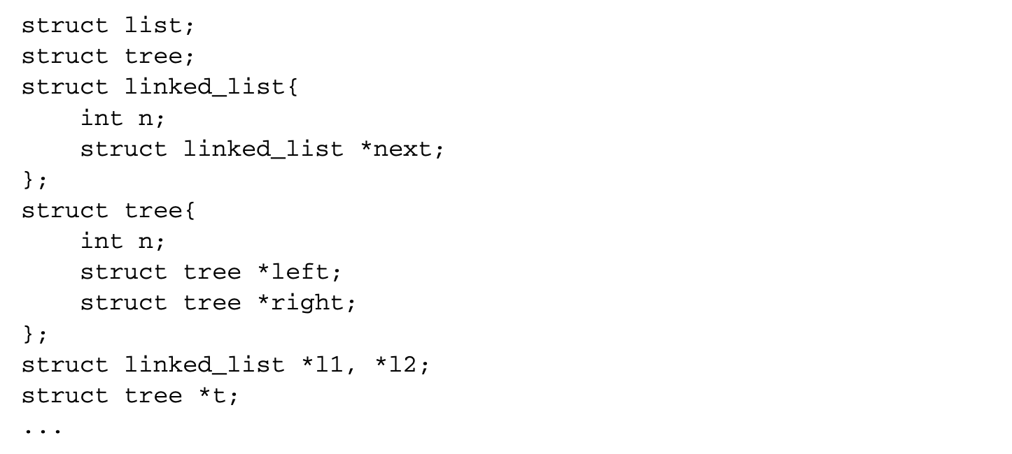 Assume that after the necessary dynamic allocations, the pointer l1 points to the head of a linked list, l2 points to the head of a different linked list, and t points to the root of a binary tree. The memory for each of these three distinct data structure instances in the program would be allocated in three distinct pools. Thus, if a single data structure instance is traversed repeatedly without accessing the other instances, the cache will not be polluted by unused data, thereby improving the cache utilization. The drawback to this technique is that it does not profile the code to identify the access patterns and hence may cause severe performance degradation when two instances, such as l1 and l2 above, are concurrently accessed.
5.8 Optimizations for Instruction Caches
Modern processors issue multiple instructions per clock cycle. To efficiently utilize this ability to issue multiple instructions per cycle, the memory system must be able to supply the processor with instructions at a high rate. This requires that the miss rate of instructions in the instruction cache be very low. Several compiler optimizations have been proposed to decrease the access latency for instructions in the instruction cache.
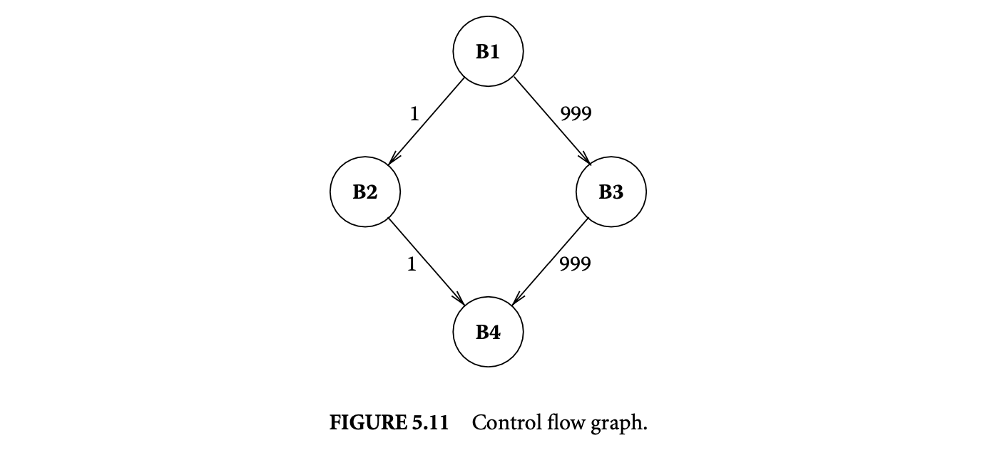
5.8.1 Code Layout in Procedures
A procedure consists of a set of basic blocks. The mapping from the basic blocks to the virtual address space can have a big impact on the instruction cache performance. Consider the section of control flow graph in Figure 5.11 that corresponds to an if-then-else statement. The numbers on the edges denote the frequency of execution of the edges. Thus, most of the time, the basic block B3 is executed after B1, and B2 is seldom executed. It is not desirable to place B2 after B1, as that could fill the cache line containing B1 with infrequently used code. The code layout algorithms use profile data to guide the mapping of basic blocks to the address space.
Figure 5.12 shows an algorithm proposed by Pettis and Hansen [22] to do profile-guided basic block layout. The algorithm sorts the edges of the control flow graph by the frequency of execution. Initially, every basic block is assumed to be in a chain containing just itself. A chain is simply a straight line path
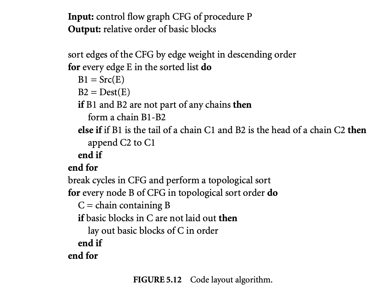 in the control flow graph. The algorithm tries to merge the chains into longer chains by looking at each edge, starting from the one with the highest frequency. If the source of the edge is the tail node of a chain and the destination is the head node of a chain, the chains are merged. This process continues until all edges are processed. Then the algorithm does a topological sort of the control flow graph after breaking cycles. The chains corresponding to the nodes in the topological order are laid out consecutively in memory.
5.8.2 Procedure Splitting
While the above algorithm separates hot blocks from cold blocks within a procedure, a poor instruction cache performance still might result. To see this, consider a program with two procedures P1 and P2. Let the hot basic blocks in each procedure occupy one cache line and the cold basic blocks occupy one cache line. If the size of the cache is two cache lines, using the layout produced by the previous algorithm might result in the hot blocks of the two procedures getting mapped to the same cache line, producing a large number of cache misses.
A simple solution to this problem is to place the hot basic blocks of different procedures close to each other. In the above example, this will avoid conflict between the hot basic blocks of the two procedures. Procedure splitting[22] is a technique that splits a procedure into hot and cold sections. Hot sections of all the procedures are placed together, and the cold sections are placed far apart from the hot sections. If the size of the entire program exceeds the cache size, while the hot sections alone fit within the cache, then procedure splitting will result in the cache being occupied by hot code for a large fraction of time. This results in very few misses during the execution of the hot code, resulting in considerable performance improvement.
Procedure splitting simply classifies the basic blocks as hot or cold based on some threshold and moves the cold basic blocks to a distant memory location. For processors that require a special instruction to jump beyond a particular distance, all branches that conditionally jump to a cold basic block are redirected to a stub code, which jumps to the actual cold basic block. Thus, the transitions between hot and cold regions have to be minimal, as they require two control transfer instructions including the costlier special jump instruction.
5.8.3 Cache Line Coloring
Another technique known to improve placement of blocks across procedures is cache line coloring [9]. Cache line coloring attempts to place procedures that call each other in such a way that they do not map to the same set of cache blocks.
Consider the following code fragment:
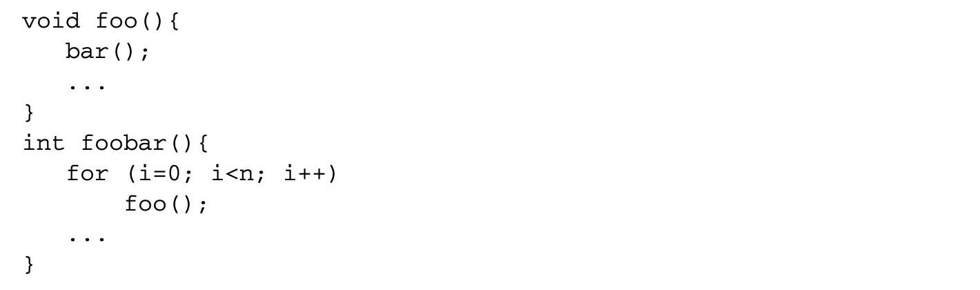
The procedure foolar contains a loop in which foo is called and foo calls bar. The procedures foo and bar must not map to the same cache line, as that will result in a large number of misses. If it is assumed that the size of the hot code blocks in the program exceeds the size of the instruction cache,procedure splitting might still result in the code blocks of foo and bar being mapped to the same set of cache lines.
The input to cache line coloring is the call graph of a program with weighted undirected edges, where the weight on the edge connecting P1 and P2 denotes the number of times P1 calls P2 or vice versa. The nodes are labeled with the number of cache lines required for that procedure. The output of the technique is a mapping between procedures to a set of cache lines. The algorithm tries to minimize the cache line conflicts between nodes that are connected by edges with high edge weights. The edges in the call graph are first sorted by their weights, and each edge is processed in the descending order of weights. If both the nodes connecting an edge have not been assigned to any cache lines, they are assigned nonconflicting cache lines. If one of the nodes is unassigned, the algorithm tries to assign nonconflicting cache lines to the unassigned node without changing the assignment of the other node. If nonconflicting colors cannot be found, it is assigned a cache line close to the other node. If both nodes have already been assigned cache lines, the technique tries to reassign colors to one of them based on several heuristics, which try to minimize the edge weight of edges connected to conflicting nodes.
The main drawback of this technique is that it only considers one level of the call depth. If there is a long call chain, the technique does not attempt to minimize conflicts between nodes in this chain that are adjacent to each other. In addition, the technique assumes that the sizes of procedures are multiples of cache line sizes, which may result in holes between procedures.
5.9 Summary and Future Directions
The various optimizations for memory hierarchies described in this chapter are essential components of optimizing compilers targeting modern architectures. While no single technique is a silver bullet for bridging the processor-memory performance gap, many of these optimizations complement each other, and their combination helps a wide range of applications. Table 5.1 summarizes how each of the optimizations achieve improved memory performance.
While these optimizations were motivated by the widening performance gap between the processor and the main memory, the recent trend of stagnant processor clock frequencies may narrow this gap. However, the stagnation of clock frequencies is accompanied by another trend -- the prevalence of chip multiprocessors (CMPs). CMPs pose a new set of challenges to memory performance and increase the importance of compiler-based memory optimizations. Compiler techniques need to focus on multi-threaded applications, as more applications will become multi-threaded to exploit the parallelism offered by CMPs. Compilers also have to efficiently deal with the changes in the memory hierarchy that may have some levels of private caches and some level of caches that are shared among the different cores. The locality in the shared levels of the hierarchy for an application is influenced by applications that are running in the other cores of the CMP.
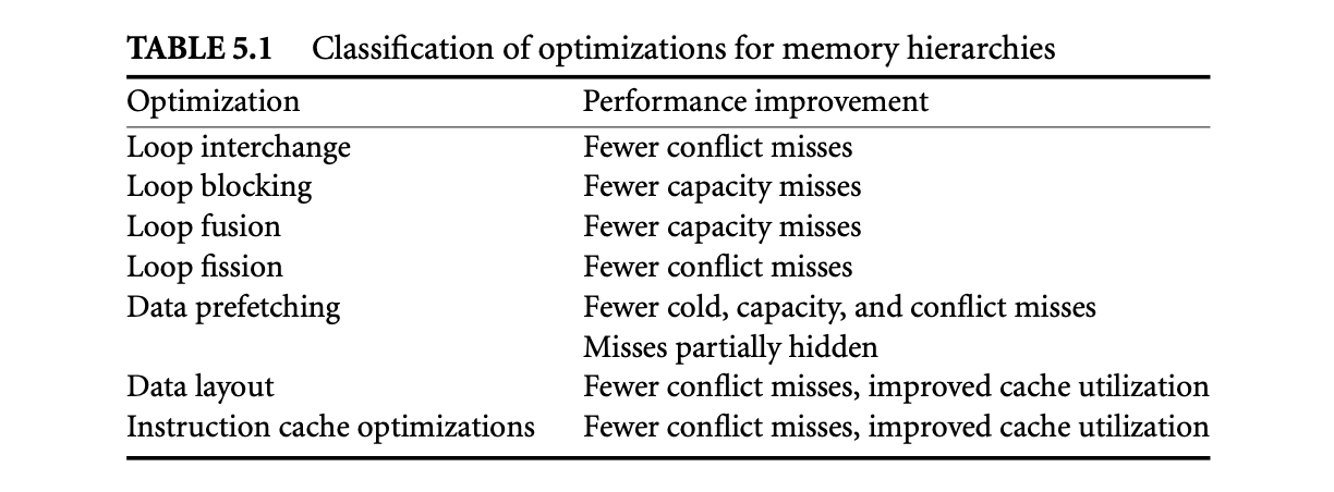
5.10 References
The work of Abu-Sufah et al. [1] was among the first to look at compiler transformations to improve memory locality. Allen and Kennedy [3] proposed the technique of automatic loop interchange. Loop tiling was proposed by Wolfe [32, 33], who also proposed loop skewing [31]. Several enhancements to tiling including tiling at the register level [11], tiling for imperfectly nested loops [2], and other improvements [12, 27] have been proposed in the literature. Wolf and Lam [29, 30] proposed techniques for combining various unimodular transformations and tiling to improve locality. Detailed discussion of various loop restructuring techniques can be found in textbooks written by Kennedy and Allen [13] and Wolfe [34] and in the dissertations of Porterfield [23] and Wolf [28].
Software prefetching was first proposed by Callahan et al. [5] and Mowry et al. [19, 20, 21]. Machine-specific enhancements to software prefetching have been proposed by Santhanam et al. [26] and Doshi et al. [8]. Luk and Mowry [15] proposed some compiler techniques to prefetch recursive data structures that may not have a strided access pattern. Saavedra-Barrera et al. [25] discuss the combined effects of unimodular transformations, tiling, and software prefetching. Mcintosh [17] discusses various compiler-based prefetching strategies and evaluates them.
Hundt et al. [10] developed an automatic compiler technique for structure layout optimizations. Calder et al. [4] and Chilimbi et al. [6, 7] proposed techniques for data object layout that require some level of programmer intervention or library support. Mcintosh et al. [18] describe an interprocedural optimization technique for placement of global values. Lattner and Adve [14] developed compiler analysis and transformation for pool allocation based on the types of data objects.
McFarling [16] first proposed optimizations targeting instruction cache performances. He gave results on optimal performance under certain assumptions. Pettis and Hansen [22] proposed several profile-guided code positioning techniques including basic block ordering, basic block layout, and procedure splitting. Hashemi et al. [9] proposed the coloring-based approach to minimize cache line conflicts in instruction caches.
References
Ken Kennedy and John R. Allen. 2002. Optimizing compilers for modern architectures: A dependence-based approach. San Francisco: Morgan Kaufmann. [19]: Todd C. Mowry. 1995. Tolerating latency through software-controlled data prefetching. PhD thesis, Stanford University, Stanford, CA.
In IPPS '96: Proceedings of the 10th International Parallel Processing Symposium, 39-45. Washington, DC: IEEE Computer Society.
Chapter 9 Types of Systems: Advances and Applications
9.1 Introduction
This chapter is about the convergence of type systems and static analysis. Historically, these two approaches to reasoning about programs have had different purposes. Type systems are developed to catch common kinds of programming errors early in the software development cycle. In contrast, static analyses were developed to automatically optimize the code generated by a compiler. The two fields also have different theoretical foundations: type systems are typically formalized as logical inference systems 1, while static analyses are typically formalized as abstract program executions 2.
Recently, however, there has been a convergence of the objectives and techniques underlying type systems and static analysis 3. On the one hand, static analysis is increasingly being used for program understanding and error detection, rather than purely for code optimization. For example, the LCLint tool 4 uses static analysis to detect null-pointer dereferences and other common errors in C programs, and it relies on type-system-like program annotations for efficiency and precision. As another example, the Error Detection via Scalable Program Analysis (ESP) tool 5 uses static analysis to detect violations of Application Programming Interface (API) usage protocols, for example, that a file can only be read or written after it has been opened.
On the other hand, type systems have become a mature and widely accepted technology. Programmers write most new software in languages such as C 6, C++ 7, Java 8, and C# 9, which all feature varying degrees of static type checking. For example, the Java type system guarantees that if a program calls a method on some object, at runtime the object will actually have a method of that name, expecting the proper number and kind of arguments. Types are also used in the intermediate languages of compilers and even in assembly languages 10, such as the typed assembly language for x86 called TALx86 11.
With this success, researchers have been motivated to explore the potential to extend traditional type systems to detect a variety of interesting classes of program errors. This exploration has shown type systems to be a robust approach to static reasoning about programs and their properties. For example, type systems have been used recently to ensure the safety of manual memory management (e.g., 12), to track andrestrict the aliasing relationships among pointers (e.g., 13), and to ensure the proper interaction of threads in concurrent programs (e.g., 14).
These new uses of type systems have brought type systems closer to the domain of static analysis, in terms of both objectives and techniques. For example, reasoning about aliasing is traditionally done via a static analysis to compute the set of may-aliases, rather than via a type system. As another example, some sophisticated uses of type systems have required making types flow sensitive15, whereby the type of an expression can change at each program point (e.g., a file's type might denote that the file is open at one point but closed at another point). This style of type system has a natural relationship to traditional static analysis, where the set of "flow facts" can change at each program point.
In this chapter, we describe two type systems that have a strong relationship to static analysis. Each of the type systems is a refinement of an existing and well-understood type system: the first refines a subset of the Java type system, while the second refines a system of simple types for the lambda calculus. The refinements are done via annotations that refine existing types to specify and check finer-grained properties. Many of the sophisticated type systems mentioned above can be viewed as refinements of existing types and type systems. Such type systems are examples of type-based analyses16; that is, they assume and leverage the existing type system and they provide information only for programs that type check with the existing type system.
In the following section we describe a type system that ensures a strong form of encapsulation in object-oriented languages. Namely, the analysis guarantees that an object of a class declared confined will never dynamically escape the class's scope. Object confinement goes well beyond the guarantees of traditional privacy modifiers such as protected and private, and it bears a strong relationship to standard static analyses.
Language designers cannot anticipate all of the refinements that will be useful for programmers or all of the ways in which these refinements can be used to practically check programs. Therefore, it is desirable to provide a framework that allows programmers to easily augment a language's type system with new refinements of interest for their applications. In Section 9.3 we describe a representative framework of this kind, supporting programmer-defined type qualifiers. A type qualifier is a simple but useful kind of type refinement consisting solely of an uninterpreted "tag." For example, C's const qualifier refines an existing type to further indicate that values of this type are not modifiable, and a nonnull qualifier could refine a pointer type to further indicate that pointers of this type are never null.
9.2 Types for Confinement
In this section we will use types to ensure that an object cannot escape the scope of its class. Our presentation is based on results from three papers on confined types17.
Background
Object-oriented languages such as Java provide a way of protecting the name of a field but not the contents of a field. Consider the following example.
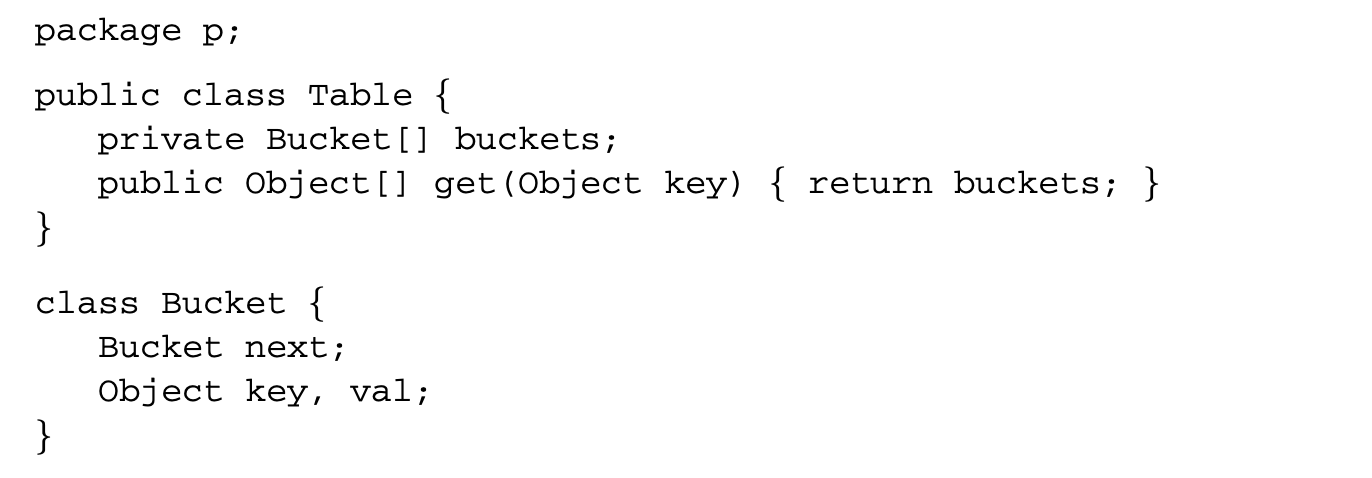
The hash table class Table is a public class that uses a package-scoped class Bucket as part of its implementation. The programmer has declared the field buckets to be private and intends the hash-table-bucket objects to be internal data structures that should not escape the scope of the Bucket class. The declaration of Bucket as packaged scoped ensures that the Bucket class is not visible outside the package p. However, even the combination of a private field and a package-scoped class does not prevent Bucket objects from being accessible outside the scope of the Bucket class. To see why, notice that the public get method in class Table has body return buckets; that provides an array of bucket objects to any client, including clients outside the package p. Any client can now update the array and thereby change the behavior of the hash table.
The example shows how an object reference can leak out of a package. Such leakage is a problem because (a) the object may represent private information such as a private key and (b) code outside the package may update the object, making it more difficult for programmers to reason about the program. The problem stems from a combination of aliasing and side effects. Aliasing occurs when an object is accessible through different access paths. In the above example, code outside the package can access bucket objects and update them.
How can we ensure that an object cannot escape the scope of its class? We will briefly discuss how one can solve the problem using static analysis and then proceed to show a type-based solution.
9.2.2 Static Analysis
Static analysis can be used to determine whether an object can escape the scope of its class. We will explain a whole-program analysis, that is, an approach that requires access to all the code in the application and its libraries.
Assuming that we have the whole program, let U be the set of class names in the program. The basic idea is to statically compute, for each expression in the program, a subset of U that conservatively approximates the possible values of . We will call that set the flow set for . For example, if the flow set for is the set , that means the expression will evaluate to either an -object, a -object, or a -object. Notice that we allow the set to be a conservative approximation; for example, might never evaluate to a -object. All we require is that if evaluates to an -object, then is a member of the flow set for .
Researchers have published many approaches to statically computing flow sets for expressions in object-oriented programs; see, for example, [2, 67, 59, 22, 2] for some prominent and efficient whole-program analyses. For the purposes of this discussion, all we rely on is that flow sets can be computed statically.
Once we have computed flow sets, for each package-scoped class we can determine whether ever appears in the flow set for an expression outside the package of . For each class that never appears in flow sets outside its package, we know its objects do not escape its package in this particular program.
The whole-program-analysis approach has several drawbacks:
Bug finding after the program is done: The approach finds bugs after the whole program is done. While that is useful, we would like to help the programmer find bugs while he or she is writing the program. No enforcement of discipline: The static analysis does not enforce any discipline on the programmer. A programmer can write crazy code, and the static analysis may then simply report that every object can escape the scope of its class. While that should be a red flag for the programmer, we would like to help the programmer determine which lines of code to fix to avoid some of the problems. Fragility: The static analysis tends to be sensitive to small changes in the program text. For one version of a program, a static analysis may find no problems with escaping objects, and then after a few lines of changes, suddenly the static analysis finds problems all over the place. We would like to help the programmer build software in a modular way such that changes in one part of the program do not affect other parts of the program.
The type-based approach in the next section has none of these three drawbacks.
The static-analysis approach in this section is one among many static analyses that solve the same or similar problems. For example, researchers have published powerful escape analyses [5, 6, 7, 27] some of which can be adapted to the problem we consider in this chapter.
9.2.3 Confined Types
We can use types to ensure that an object cannot escape the scope of its class. We will show an approach for Java that extends Java with the notions of confined type and anonymous method. The idea is that if we declare a class to be confined, the type system will enforce rules that ensure that an object of the class cannot escape the scope of the class. If a program type checks in the extended type system, an object cannot escape the scope of its class.
Confinement can be enforced using two sets of constraints. The first set of constraints, confinement rules, applies to the classes defined in the same package as the confined class. These rules track values of confined types and ensure that they are neither exposed in public members nor widened to nonconfined types. The second kind of constraints, anonymity rules, applies to methods inherited by the confined classes, potentially including library code, and ensures that these methods do not leak a reference to the distinguished variable this, which may refer to an object of confined type.
We will discuss the confinement and anonymity rules next and later show how to formalize the rules and integrate them into the Java type system.
9.2.3.1 Confinement Rules
The following confinement rules must hold for all classes of a package containing confined types.
- : A confined type must not appear in the type of a public (or protected) field or the return type of a public (or protected) method.
- : A confined type must not be public.
- : Methods invoked on an expression of confined type must either be defined in a confined class or be anonymous.
- : Subtypes of a confined type must be confined.
- : Confined types can be widened only to other confined types.
- : Overriding must preserve anonymity of methods.
Rule prevents exposure of confined types in the public interface of the package, as client code could break confinement by accessing values of confined types through a type's public interface. Rule is needed to ensure that client code cannot instantiate a confined class. It also prevents client code from declaring field or variables of confined types. The latter restriction is needed so that code in a confining package will not mistakenly assign objects of confined types to the fields or variables outside that package. Rule ensures that methods invoked on an object enforce confinement. In the case of methods defined in the confining package, this ensues from the other confinement rules. Inherited methods defined in another package do not have access to any confined fields, since those are package scoped (rule ). However, an inherited method of confined class may leak the this reference, which is implicitly widened to the method's declaring class. To prevent this, rule requires these methods to be anonymous (as explained below). Rule prevents the declaration of a public subclass of a confined type. This prevents spoofing leaks, where a public subtype defined outside of the confined package is used to access private fields 18. Rule prevents code within confining packages from assigning values of confined types to fields or variables of public types. Finally, rule allows us to statically verify the anonymity of the methods that are invoked on expressions of confined types.
9.2.3.2 Anonymity Rule
The anonymity rule applies to inherited methods that may reside in classes outside of the enclosing package. This rule prevents a method from leaking the this reference. A method is anonymous if it has the following property.
- : The this reference is used only to select fields and as the receiver in the invocation of other anonymous methods.
This prevents an inherited method from storing or returning this as well as using it as an argument to a call. Selecting a field is always safe, as it cannot break confinement because only the fields visible in the current class can be accessed. Method invocation (on this) is restricted to other methods that are anonymous as well. Note that we check this constraint assuming the static type of this, and rule ensures that the actual method invoked on this will also be anonymous. Thus, rule ensures that the anonymity of a method is independent of the result of method lookup.
Rule could be weakened to apply only to methods inherited by confined classes. For instance, if an anonymous method m of class is overridden in both class B and C, and B is extended by a confined class while C is not, then the method m in B must be anonymous while m of C need not be. The reason is that the method m of C will never be invoked on confined objects, so there is no need for it to be anonymous.
9.2.3.3 Confined Featherweight Java
Confined Featherweight Java (ConfinedFJ) is a minimal core calculus for modeling confinement for a Java-like object-oriented language. ConfinedFJ extends Featherweight Java (FJ), which was designed by Igarashi et al. 19 to model the Java type system. It is a core calculus, as it limits itself to a subset of the Java language with the following five basic expressions: object construction, method invocation, field access, casts, and local variable access. This spartan setting has proved appealing to researchers. ConfinedFJ stays true to the spirit of FJ. The surface differences lie in the presence of class- and method-level visibility annotations. In ConfinedFJ, classes can be declared to be either public or confined, and methods can optionally be declared as anonymous. One further difference is that ConfinedFJ class names are pairs of identifiers bundling a package name and a class name just as in Java.
9.2.3.4 Syntax
Let metavariable L range over class declarations, range over a denumerable set of class identifiers, range over constructor and method declarations, respectively, and and range over field names and variables (including parameters and the pseudo-variable this), respectively. Let range over expressions and range over values.
We adopt FJ notational idiosyncrasies and use an overbar to represent a finite (possibly empty) sequence. We write to denote the sequence and similarly for and . We write to denote , to denote , and finally to denote .
The syntax of ConfinedFJ is given in Figure 9.1. An expression can be either one of a variable (including this), a field access e.f, a method invocation , a cast (C) e, or an object new . Since ConfinedFJ has a call-by-value semantics, it is expedient to add a special syntactic form for fully evaluated objects, denoted new .
Class identifiers are pairs p.q such that p and q range over denumerable disjoint sets of names. For ConfinedFJ class name p.q, p is interpreted as a package name and q as a class name. In ConfinedFJ, class identifiers are fully qualified. For a class identifier C, denotes the identifier's package prefix, so, for example, the value of is p.
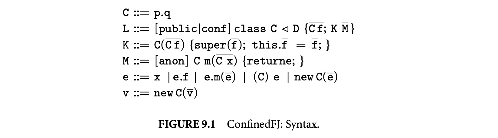
Each class declaration is annotated with one of the visibility modifiers public, conf, or none; a public class is declared by public class , a package-scoped, confined class is conf class , and a package-scoped, nonconfined class is class . Methods can be annotated with the optional anon modifier to denote anonymity.
We will not formalize the dynamic semantics of ConfinedFJ (for full details, see 20). We assume a class table that stores the definitions of all classes of the ConfinedFJ program such that is the definition of class C. The subtyping relation C <: D denotes that class C is a subtype of class D; <: is the smallest reflexive and transitive class ordering that has the property that if C extends D, then C <: D. Every class is a subtype of l.Object. The function returns the list of all fields of the class C including inherited ones; returns the list of all methods in the class C; returns the identifier of defining class for the method m.
9.2.3.5 Type Rules
Figure 9.2 defines relations used in the static semantics. The predicate holds if the class table maps C to a class declared as confined. Similarly, the predicate holds if the class table maps C to a class declared as public. The function yields the type signature of a method. The predicate holds if m is a valid, anonymity-preserving redefinition of an inherited method or if this is the method's original definition. Class visibility, written , states that a class C is visible from D if C is public or if both classes are in the same package.
The safe subtyping relation, written C D, is a confinement-preserving restriction of the subtyping relation <:. A class C is a safe subtype of D if C is a subtype of D and either C is public or D is confined. This relation is used in the typing rules to prevent widening a confined type to a public type; confinement-preserving widening requires safe subtyping to hold. The type system further constrains subtyping by enforcing that all subclasses of a confined class must belong to the same package (see the T-Class rule and the definition of visibility in Figure 9.4). Notice that safe subtyping is reflexive and transitive.
Figure 9.3 defines constraints imposed on anonymous methods. A method m is anonymous in class C, written , if its declaration is annotated with the anon modifier. The following syntactic restrictions are imposed on the body of an anonymous method. An expression e is anonymous in class C, written , if the pseudo-variable this is used solely for field selection and anonymous method invocation. (C) e is anonymous if e is anonymous. new C() and e.m() are anonymous if e this and
Confined types, type visibility, and safe subtyping:

Method type lookup:
 Valid method overriding:
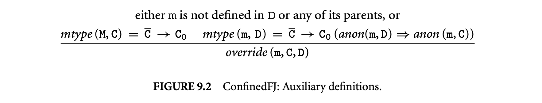
Anonymous method:
 Anonymity constraints:
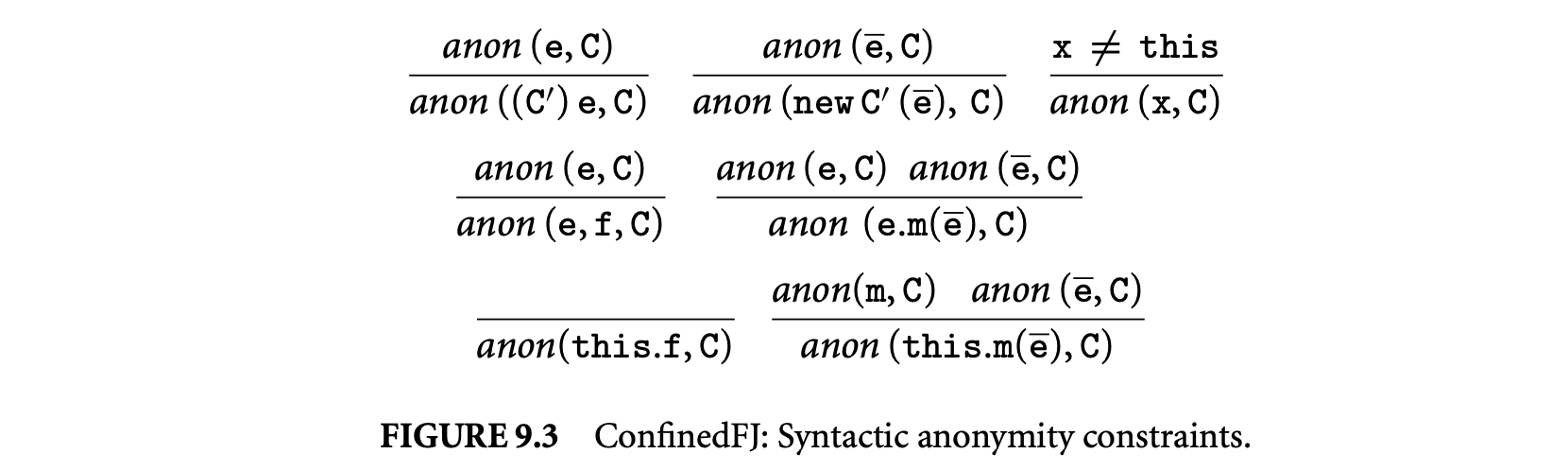
are anonymous. With the exception of this all variables are anonymous. this.f is always anonymous, and this.m() is anonymous in if is anonymous in and is anonymous. We write \mbox{\it anon}(\overline{\mathtt{e}},\mathtt{C}) to denote that all expressions in are anonymous.
9.2.3.6 Expression Typing Rules
The typing rules for ConfinedFJ are given in Figure 9.4, where type judgments have the form , in which is an environment that maps variables to their types. The main difference with is that these rules disallow unsafe widening of types. This is captured by conditions of the form that enforce safe subtyping:
- Rules T-Var and T-Field are standard.
- Rule T-New prevents instantiating an object if any of the object's fields with a public type is given a confined argument. That is, for fields with declared types and argument types , relation must hold. By definition of , if is confined, then is confined as well.
- Rule T-Invk prevents widening of confined arguments to public parameters by enforcing safe subtyping of argument types with respect to parameter types. To prevent implicit widening of the receiver, we consider two cases. Assume that the receiver has type and the method is defined in ; then it must be the case either that is a safe subtype of or that has been declared anonymous in .
- Rule T-UCast prevents casting a confined type to a public type. Notice that a down cast preserves confinement because by rule T-Class a confined class can only have confined subclasses.
9.2.3.7 Typing Rules for Methods and Classes
Figure 9.4 also gives rules for typing methods and classes:
- Rule T-Method places the following constraints on a method defined in class with body . The type D of must be a safe subtype of the method's declared type . The method must preserve anonymity declarations. If is declared anonymous, must comply with the corresponding restrictions. The most interesting constraint is the visibility enforced on the body by \Gamma\vdash\mbox{\it visible}(\mathtt{e},\mathtt{C}_{0}), which is defined recursively over the structure of terms. It ensures that the types of all subexpressions of are visible from the defining class . In particular, the method parameters used in the method body must have types visible in .
- Rule T-Class requires that if class extends , then must be visible in , and if is confined, then so is . Rule T-Class allows the fields of a class to have types not visible in , but the constraint of \Gamma\vdash\mbox{\it visible}(\mathtt{e},\mathtt{C}) in rule T-Method prohibits the method of from accessing such fields.
Expression typing:
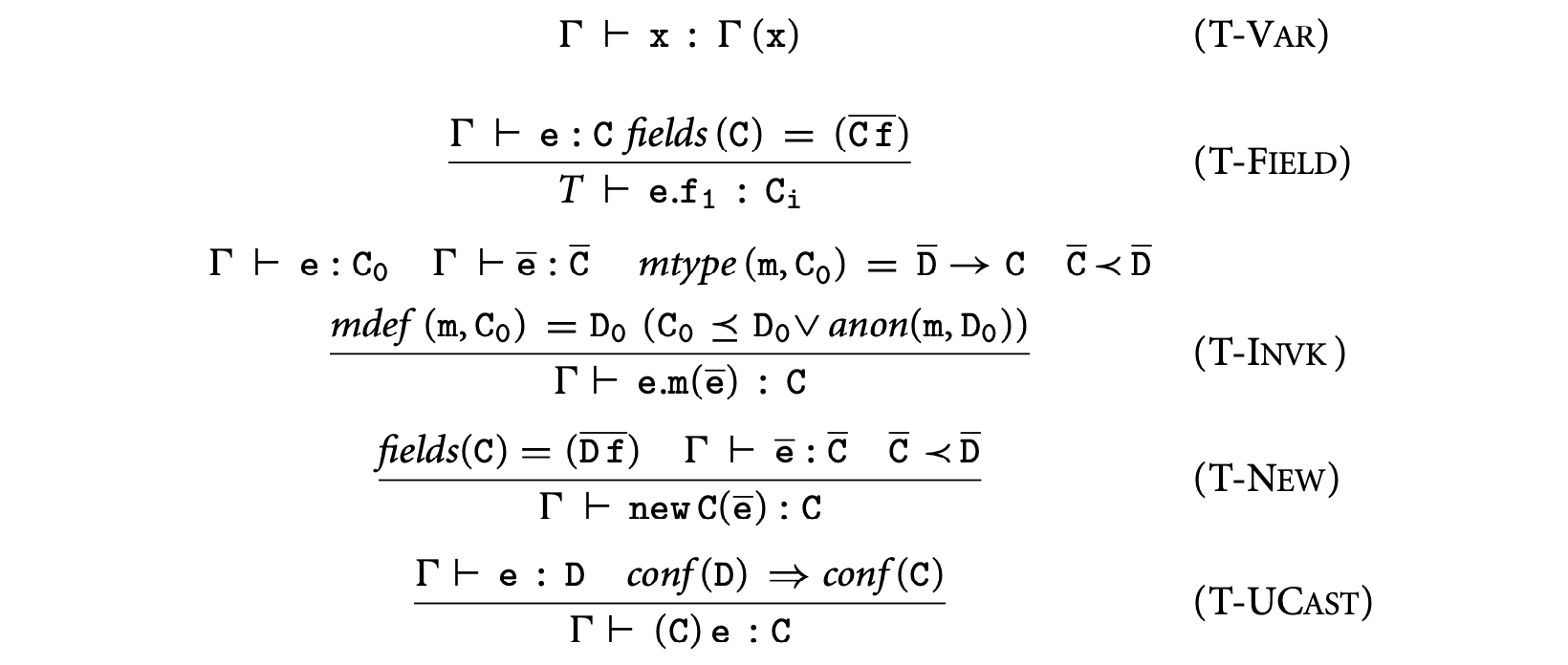
Method typing:
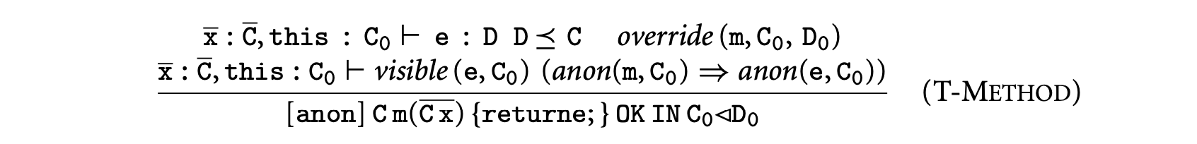 Class typing:
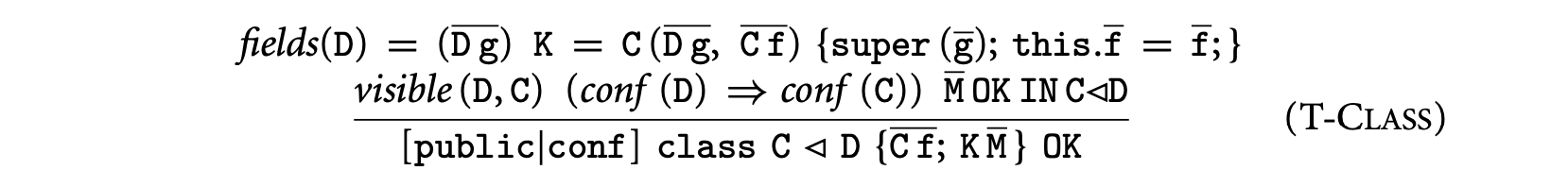 Static expression visibility:
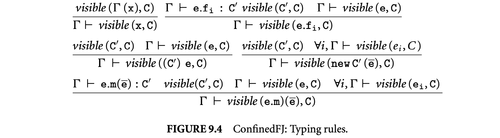 The class table CT is well-typed if all classes in CT are well-typed. For the rest of this paper, we assume CT to be well-typed.
9.2.3.8 Relation to the Informal Rules
We now relate the confinement and anonymity rules with the ConfinedFJ type system. The effect of rule , which limits the visibility of fields if their type is confined, is obtained as a side effect of the visibility constraint as it prevents code defined in another package from accessing a confined field. ConfinedFJ could be extended with a field and method access modifier without significantly changing the type system. The expression typing rules enforce confinement rules and by ensuring that methods invoked on an object of confined type are either anonymous or defined in a confined class and that widening is confinement preserving. Rule uses access modifiers to limit the use of confined types, and the same effect is achieved by the visibility constraint on the expression part of T-METHOD. Rule , which states that subclassing is confinement preserving, is enforced by T-CLASs. Rule , which states that overriding is anonymity preserving, is enforced by T-METHOD. Finally, the anonymity constraint of rule is obtained by the anon predicate in the antecedent of T-METHOD.
9.2.3.9 Two ConfinedFJ Examples
Consider the following stripped-down version of a hash table class written in ConfinedFJ. The hash table is represented by a class p.Table defined in some package p that holds a single bucket of class p.Buck. The bucket can be obtained by calling the method get() on a table, and the bucket's data can then be obtained by calling getData(). In this example, buckets are confined, but they extend a public class p.Cell. The interface of p.Table.get() specifies that the method's return type is p.Cell; this is valid, as that class is public. In this example a factory class, named p.Factory, is needed to create instances of p.Table. because the table's constructor expects a bucket and since buckets are confined, they cannot be instantiated outside of their defining package.
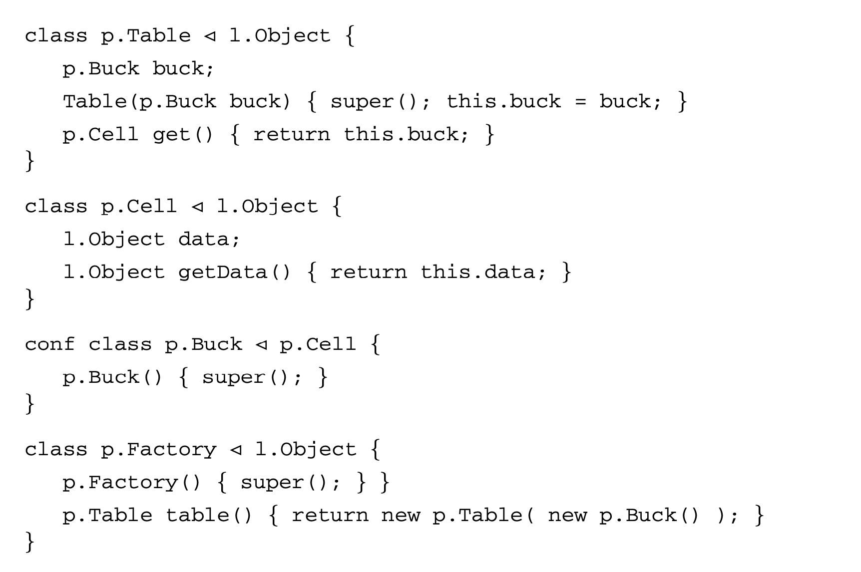 This program does not preserve confinement as the body of the p.Table.get() method returns an instance of a confined class in violation of the widening rule. The breach can be exhibited by constructing a class o.Breach in package o that creates a new table and retrieves its bucket.
 The expression new
 o.Breach().main() eventually evaluates to new p.Buck(), exposing the confined class to code defined in another package. This example is not typable in the ConfinedFJ type system. The method p.Table.get() does not type-check because rule T-Method requires the type of the expression returned by the method to be a safe subtype of the method's declared return type. The expression has the confined type p.Buck, while the declared return type is the public type p.Cell.
In another prototypical breach of confinement, consider the following situation in which the confined class p.Self extends a Broken parent class that resides in package o. Assume further that the class inherits its parent's code for the reveal() method.
Inspection of this code does not reveal any breach of confinement, but if we widen the scope of our analysis to the o.Broken class, we may see
 Invoking
 reveal() on an instance of p.Self will return a reference to the object itself. This does not type-check because the invocation of reveal() in p.Main.get() violates the rule T-Invk (because the non-anonymous method reveal(), inherited from a public class o.broken, is invoked on an object of a confined type p.Self). The method reveal() cannot be declared anonymous, as the method returns this directly.
9.2.3.10 Type Soundness
Zhao et al. 21 presented a small-step operational semantics of ConfinedFJ, which is a computation-step relation on program states , . They define that a program state satisfies confinement if every object is in the scope of its defining class. They proceed to prove the following type soundness result (for a version of ConfinedFJ without downcast).
Theorem (confinement) 21: If is well-typed, satisfies confinement, and , then satisfies confinement.
The confinement theorem states that a well-typed program that initially satisfies confinement preserves confinement. Intuitively, this means that during the execution of a well-typed program, all the objects that are accessed within the body of a method are visible from the method's defining package. The only exception is for anonymous methods, as they may have access to this, which can evaluate to an instance of a class confined in another package, and if this occurs the use of this is restricted to be a receiver object.
Confined types have none of the three drawbacks of whole-program static analysis: we can type-check fragments of code well before the entire program is done, the type system enforces a discipline that can help make many types confined, and a change to a line of code only affects types locally.
9.2.3.11 Confinement Inference
Every type-correct FJ program can be transformed into a type-correct ConfinedFJ program by putting all the classes into the same package. Conversely, every type-correct ConfinedFJ program can be transformedinto a type-correct Java program by removing all occurrences of the modifiers and . (The original version of FJ does not have packages.)
The modifiers and can help enforce more discipline than Java does. If we begin with a program in FJ extended with packages and want to enforce the stricter discipline of ConfinedFJ, we face what we call the confinement inference problem.
The confinement inference problem: Given a Java program, find a subset of the package-scoped classes that we can make confined and find a subset of the methods that we can make anonymous.
The confinement inference problem has a trivial solution: make no classes confined and make no method anonymous. In practice we may want the largest subsets we can get.
Grothoff et al. 22 studied confinement inference for a variant of the confinement and anonymity rules in this chapter. They used a constraint-based program analysis to infer confinement and method anonymity. Their constraint-based analysis proceeds in two steps: (a) generate a system of constraints from program text and then (b) solve the constraint system. The constraints are of the following six forms:
 A constraint \mathsf{not\mbox{-}anon}(\mathsf{methodId}) asserts that the method methodId is not anonymous; similarly, \mathsf{not\mbox{-}conf}(\mathsf{classId}) asserts that the class classId is not confined. The remaining four forms of constraints denote logical implications. For example, not-anon() not-conf (C) is read "if method in class is not anonymous, then class will not be confined."
From each expression in a program, we generate one or more constraints. For example, for a type expression for which the static Java type of is , we generate the constraint \mathsf{not\mbox{-}conf}(\mathtt{C})\Rightarrow\mathsf{not\mbox{-}conf}( \mathtt{D}), which represents the condition from the T-UCast rule that .
All the constraints are ground Horn clauses. The solution procedure computes the set of clauses \mathsf{not\mbox{-}conf}(\mathsf{classId}) that are either immediate facts or derivable via logical implication. This computation can be done in linear time 23 in the number of constraints, which, in turn, is linear in the size of the program.
A solution represents a set of classes that cannot be confined and a set of methods that are not anonymous. The complements of those sets represent a maximal solution to the confinement inference problem.
Grothoff et al. 22 presented an implementation of their constraint-based analysis. They gathered a suite of 46,000 Java classes and analyzed them for confinement. The average time to analyze a class file is less than 8 milliseconds. The results show that, without any change to the source, 24% of the package-scoped classes (exactly 3,804 classes, or 8% of all classes) are confined. Furthermore, they found that by using generic container types, the number of confined types could be increased by close to 1,000 additional classes. Finally, with appropriate tool support to tighten access modifiers, the number of confined classes can be well over 14,500 (or over 29% of all classes) for that same benchmark suite.
9.2.4 Related Work on Alias Control
The type-based approach in this chapter is one among many type-based approaches that solve the same or similar problems. For example, a popular approach is to use a notion of ownership type 24 for controlling aliasing. The basic idea of ownership types is to use the concept of domination on the dynamic object graph. (In a graph with a starting vertex , a vertex dominates another vertex if every path from to must pass through .) In a dynamic object graph, we may have an object we think of as owning several representation objects. The goal of ownership types is to ensure that the owner object dominates the representation objects. The dominance relation guarantees that the only way we can access a representation object is via the owner. An ownership type system has type rules that are quite different than the rules for confined types.
9.3 Type Qualifiers
In this section we will use types to allow programmers to easily specify and check desired properties of their applications. This is achieved by allowing programmers to introduce new qualifiers that refine existing types. For example, the type nonzero int is a refinement of the type int that intuitively denotes the subset of integers other than zero.
9.3.1 Background
Static type systems are useful for catching common programming errors early in the software development cycle. For example, type systems can ensure that an integer is never accidentally used as a string and that a function is always passed the right number and kinds of arguments. Unfortunately, language designers cannot anticipate all of the program errors that programmers will want to statically detect, nor can they anticipate all of the practical ways in which such errors can be detected.
As a simple example, while most type systems in mainstream programming languages can distinguish integers from strings and ensure that each kind of data is used in appropriate ways, these type systems typically cannot distinguish positive from negative integers. Such an ability would enable stronger assurances about a program, for example, that it never attempts to take the square root of a negative number. As another example, most type systems cannot distinguish between data that originated from one source and data that originated from a different source within the program. Such an ability could be useful to track a form of value flow, for example, to ensure that a string that was originally input from the user is treated as tainted and therefore given restricted capabilities (e.g., such a string should be disallowed as the format-string argument to C's printf function, since a bad format string can cause program crashes and worse).
Without static checking for these and other kinds of errors, programmers have little recourse. They can use assert statements, which catch errors, but only as they occur in a running system. They can specify desired program properties in comments, which are useful documentation but need have no relation to the actual program behavior. In the worst case, programmers simply leave the desired program properties completely implicit, making these properties easy to misunderstand or forget entirely.
9.3.2 Static Analysis
Static analysis could be used to ensure desired program properties and thereby guarantee the absence of classes of program errors. Indeed, generic techniques exist for performing static analyses of programs (e.g., 2), which could be applied to the properties of interest to programmers. As with confinement, one standard approach is to compute a flow set for each expression in the program, which conservatively overapproximates the possible values of . However, instead of using class names as the elements of a flow set, each static analysis defines its own domain of flow facts.
For example, to track positive and negative integers, a static analysis could use a domain of signs 25, consisting of the three elements , , and with the obvious interpretations. If the flow set computed for an expression contains only the element , we can be sure that will evaluate to a positive integer. In our format-string example, a static analysis could use a domain consisting of the elements tainted and untainted, representing, respectively, data that do and do not come from the user. If the flow set computed for an expression contains only the element untainted, we can be sure that does not come from the user.
While this approach is general, it suffers from the drawbacks discussed in Section 9.2.2. First, whole-program analysis is typically required for precision, so errors are only caught once the entire program has been implemented. Second, the static analysis is descriptive, reporting the properties that are true of a given program, rather than prescriptive, providing a discipline to help programmers achieve the desired properties. Finally, the results of a static analysis can be sensitive to small changes in the program.
 The type-based approach described next is less precise than some static analyses but has none of the above drawbacks.
9.3.3 A Type System for Qualifiers
We now develop a type system that supports programmer-defined type qualifiers. After a brief review of the simply typed lambda calculus, types are augmented with user-defined tags and language support for tag checking. A notion of subtyping for tagged types provides a natural form of type qualifiers. Finally, more expressiveness is achieved by allowing users to provide specialized typing rules for qualifier checking.
9.3.3.1 Simply Typed Lambda Calculus
We assume familiarity with the simply typed lambda calculus and briefly review the portions that are relevant for the rest of the section. Many other sources contain fuller descriptions of the simply typed lambda calculus, for example, the text by Pierce 1.
Figure 9.5 shows the syntax for the simply typed lambda calculus augmented with integers and integer addition. The metavariable ranges over types, and ranges over expressions. The syntax denotes the type of functions with argument type and result type . The metavariable ranges over integer constants, and ranges over variable names. The syntax : represents a function with formal parameter (of type ) and body , and the syntax represents application of the function expression to the actual argument .
Figure 9.6 presents static typechecking rules for the simply typed lambda calculus. The rules define a judgment of the form : . The metavariable ranges over type environments, which are finite mappings from variables to types. Informally, the judgment : says that expression is well-typed with type under the assumption that free variables in have the types associated with them in . The rules in Figure 9.6 are completely standard.
Static type-checking enforces a notion of well-formedness on programs at compile time, thereby preventing some common kinds of runtime errors. For example, the rules in Figure 9.6 ensure that a well-typed expression (with no free variables) will never attempt to add an integer to a function at runtime. A type system's notion of well-formedness is formalized by a type soundness theorem,
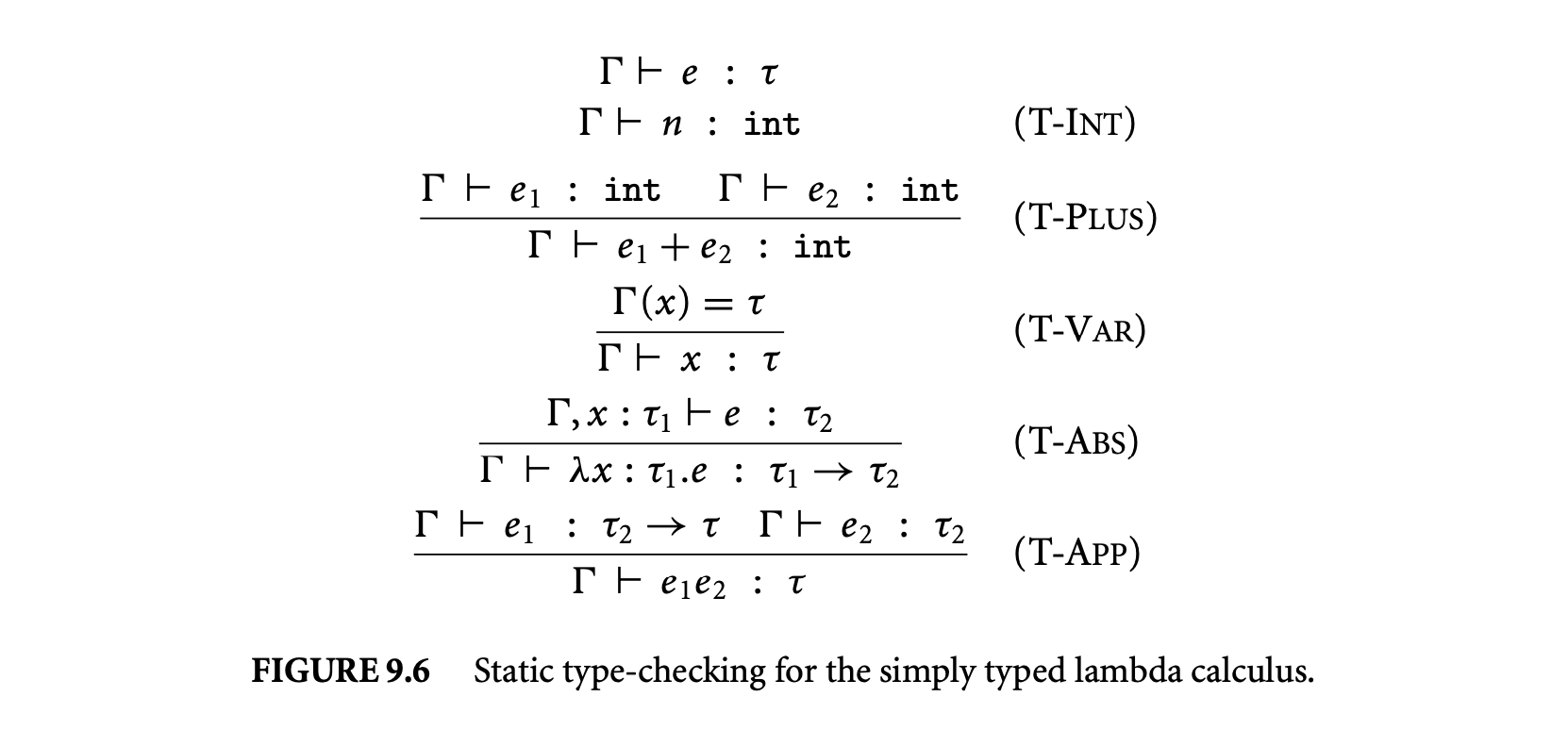

which specifies the properties of well-typed programs. Intuitively, type soundness for the simply typed lambda calculus says that the evaluation of well-typed expressions will not "get stuck," which happens when an operation is attempted with operand values of the wrong types.
A type soundness theorem relies on a formalization of a language's evaluation semantics. There are many styles of formally specifying language semantics and of proving type soundness, and common practice today is well described by others 26. These topics are beyond the scope of this chapter.
9.3.3.2 Tag Checking
One way to allow programmers to easily extend their type system is to augment the syntax for types with a notion of programmer-defined type tags (or simply tags). The new syntax of types is shown in Figure 9.7. The metavariable ranges over an infinite set of programmer-definable type tags. Each type is now augmented with a tag. For example, positive int could be a type, where positive is a programmer-defined tag denoting positive integers. Function types include a top-level tag as well as tags for the argument and result types.
For programmers to convey the intent of a type tag, the language is augmented with two new expression forms, as shown in Figure 9.7. Our presentation follows that of Foster et al. 27. The expression evaluates and tags the resulting value with . For example, if the expression evaluates to a string input by the user, one can use the expression to declare the intention to consider 's value as tainted 28. The expression evaluates and checks that the resulting value is tagged with . For example, the expression ensures that 's value does not originate from the user and is therefore an appropriate format-string argument to . A failed causes the program to terminate erroneously.
Just as our base type system in Figure 9.6 statically tracks the type of each expression, so does our augmented type system, using the augmented syntax of types. The rules are shown in Figure 9.8. For simplicity, the rules are set up so that each runtime value created during the program's execution will have
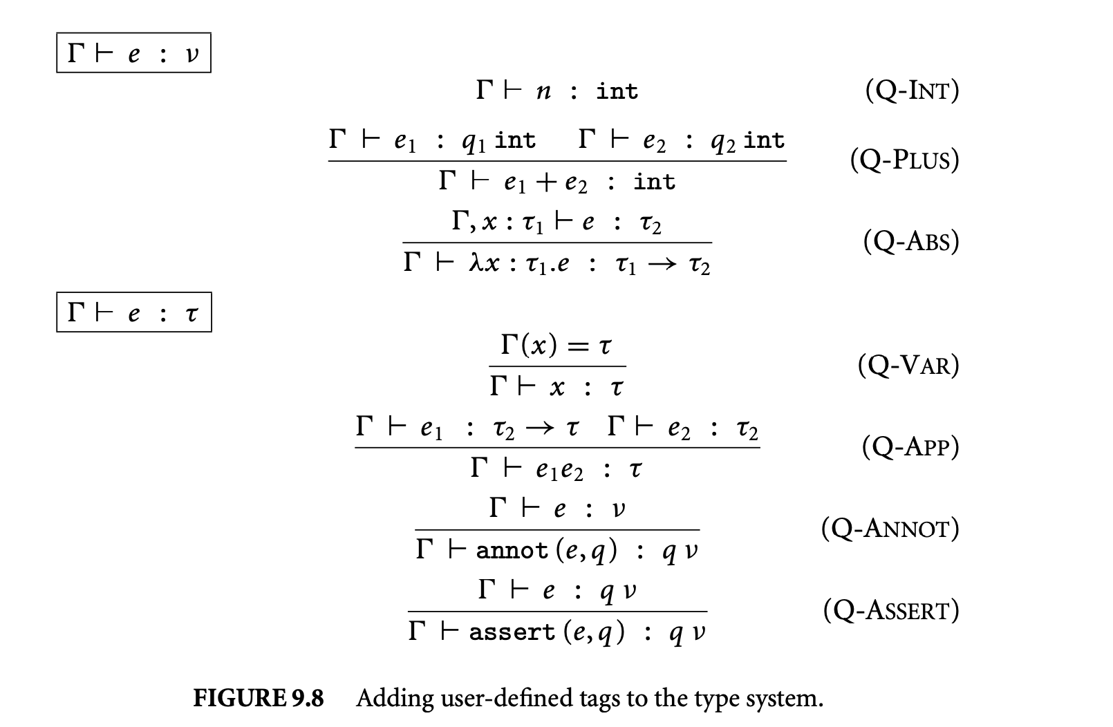
exactly one tag (a conceptually untagged value can be modeled by tagging it with a distinguished notag tag). This invariant is achieved via two interrelated typing judgments. The judgment determines an untagged type for a given expression. This judgment is only defined for constructor expressions, which are expressions that dynamically create new values. The judgment is the top-level type-checking judgment. It is defined for all other kinds of expressions. The Q-Annot rule provides a bridge between the two judgments, requiring each constructor expression to be tagged in order to be given a complete type .
Intuitively, the type system conservatively ensures that if holds, the value of at run time will be tagged with . The rules for and are straightforward: Q-Annot includes as the tag on the type of , while Q-Assett requires that 's type already includes the tag . The rest of the rules are unchanged from the original simply typed lambda calculus, except that the premises of Q-Plus allow for the tags on the types of the operands. Nonetheless, these unchanged rules have exactly the desired effect. For example, Q-App requires the actual argument's type in a function application to match the formal argument type, thereby ensuring that the function only ever receives values tagged with the expected tag.
Together the rules in Figure 9.8 provide a simple form of value-flow analysis, statically ensuring that values of a given tag will flow at runtime only to places where values of that tag are expected. For example, a programmer can define a square-root function of the form

and the type system guarantees that only values explicitly tagged as positive will be passed to the function. As another example, the programmer can statically detect possible division-by-zero errors by replacing each divisor expression (assuming our language included integer division) with the expression assert(, nonzero). Finally, the type of the following function has type tainted intuntainted int which ensures that although the function accepts a tainted integer as an argument, this integer does not flow to the return value:

However, the following function, which returns the given tainted argument, is forced to record this fact in its type, tainted inttainted int:

9.3.3.2.1 Type Soundness
The notion of type soundness in the presence of tags is a natural extension of that of the simply typed lambda calculus. Type soundness still ensures that well-typed expressions will not get stuck, but the notion of stuckness now includes failed asserts. This definition of stuckness formalizes the idea that tagged values will only flow where they are expected. Type soundness can be proven using standard techniques.
9.3.3.2.2 Tag Inference
It is possible to consider tag inference for our language. Constructor expressions are no longer explicitly annotated via annot, and formal argument types no longer include tags. Tag inference automatically determines the tag of each constructor expression and the tags on each formal argument or determines that the program cannot be typed. Programmers still must employ assert explicitly to specify constraints on where values of particular tags are expected.
As with confinement inference, a constraint-based program analysis can be used for tag inference. Conceptually, each subexpression in the program is given its own tag variable, and the analysis then generates equality constraints based on each kind of expression. For example, in a function application, the tag of the actual argument is constrained to match the tag of the formal argument type. The simple equality constraints generated by tag inference can be solved in linear time 29. Furthermore, if the constraints have a solution, there exists a principal solution, which is more general than every other solution. Intuitively, this is the solution that produces the largest number of tags.
For example, consider the following function:
 One possible typing for the function gives both and the type tainted int. However, a more precise typing gives 's type a fresh tag , since the function's constraints do not require it to have the tag tainted. This new typing encodes that fact as well as the fact that and flow to disjoint places in the program. Finally, the following program generates constraints that have no solution, since is required to be both tainted and untainted:

9.3.3.3 Qualifier Checking
While the type system in the previous subsection allows programmers to specify and check new properties of interest via tags, its expressiveness is limited because tags are completely uninterpreted. For example, the type system does not "know" the intent of tags such as positive, nonzero, tainted, and untainted; it only knows that these tags are not equivalent to one another. However, tags often have natural relationships to one another. For example, intuitively it should be safe to pass a positive int where a nonzero int is expected, since a positive integer is also nonzero. Similarly, we may want to allow untainted data to be passed where tainted data is expected, since allowing that cannot cause tainted data to be improperly used. The type system of the previous section does not permit such flexibility.
Foster et al. observed that this expressiveness can be naturally achieved by allowing programmers to specify a partial order on type tags 27. Intuitively, if , then denotes a stronger constraint than . The programmer can now declare positive nonzero and, similarly, untainted tainted, where untainted denotes the set of values that are definitely untainted, and tainted now denotes the set of values that are possibly tainted. The programmer-defined partial order naturally induces a subtyping relation among tagged types. For example, given the above partial order, positive int would be considered a subtype of nonzero int, which therefore allows a value of the former type to be passed where a value of the latter type is expected.
With this added expressiveness, type tags can be considered full-fledged type qualifiers. For example, a canonical example of a type qualifier is C's const annotation, which indicates that the associated value can be initialized but not later updated. C allows a value of type int* to be passed where a (const int) * is expected. This is safe because it simply imposes an extra constraint on the given pointer value, namely, that its contents are never updated. However, a value of type (const int) * cannot safely be passed where an int* is expected, since this would allow the pointer value's constness to be forgotten, allowing its contents to be modified. Another useful example qualifier is nonnull for pointers, whereby it is safe to pass a nonnull pointer where an arbitrary pointer is expected, but not vice versa.
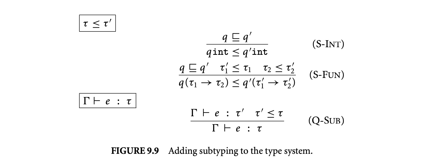
The subtyping relation depends on the partial order among qualifiers in a straightforward way. As usual, subtyping is contravariant on function argument types for soundness 30.
As an example of this type system in action, consider an expression of type positive int. Assuming that the programmer specifies positive nonzero, then by S-Int we have positive int and by Q-Sub we have nonzero int. Therefore, by the Q-App rule from Figure 9.8, may be passed to a function expecting an argument of type nonzero int.
As an aside, the addition of subtyping makes our formal system expressive enough to encode multiple qualifiers per type. For example, to encode a type like untainted positive int, one can define a new qualifier, untainted_positive, along with the partial-order untainted_positive untainted and untainted_positive positive. Then the subtyping and subsumption rules allow an untainted_positive value to be treated as being both untainted and positive, as desired.
As before, type soundness says that the type system guarantees that all asserts will succeed at runtime, where the runtime assertion check now requires a value's associated qualifier to be "less than" the specified qualifier, according to the declared partial order. The type soundness proof again uses standard techniques. It is also possible to generalize tag inference to support qualifier inference. The approach is similar to that described above, although the generated constraints are now subtype constraints instead of equality constraints.
Foster's thesis discusses type soundness and qualifier inference in detail 31. It also discusses CQUAL, an implementation of programmer-defined type qualifiers that adapts the described theory to the C language. CQUAL has been used successfully for a variety of applications, including inference of constness 32, detection of format-string vulnerabilities 33, detection of user/kernel pointer errors 34, validation of the placement of authorization hooks in the Linux kernel 35, and the removal of sensitive information from crash reports 36.
9.3.3.4 Qualifier-Specific Typing Rules
Qualifier-Specific Typing RulesThe partial order allows programmers to specify more information about each qualifier, making the overall type system more flexible. However, most of the intent of a qualifier must still be conveyed indirectly via annots, which is tedious and error prone. For example, the programmer must use annot to explicitly annotate each constructor expression that evaluates to a positive integer as being positive, or else it will not be considered as such by the type system. Therefore, the programmer has the burden of manually figuring out which expressions are positive and which are not. Furthermore, if the programmer accidentally annotates an expression such as -34 + 5 as positive, the type system will happily allow this expression to be passed to a square-root function expecting a positive int, even though that will likely cause a runtime error.
Qualifier inference avoids the need for explicit annotations using annot. However, qualifier inference simply determines which expressions must be treated as positive to satisfy a program's asserts. There is no guarantee that these expressions actually evaluate to positive integers, and many expressions that do evaluate to positive integers will not be found to be positive by the inferencer.
To address the burden and fragility of qualifier annotations, we consider an alternate approach to expressing a qualifier's intent. Instead of relying on program annotations, we require qualifier designers to specify a programming discipline for each qualifier, which indicates when an expression may be given that qualifier. For example, a programming discipline for positive might say that all positive constants can be considered positive and that an expression of the form can be considered positive if each operand expression can itself be considered positive according to the discipline. In this way, the discipline declaratively expresses the fact that 34 + 5 can be considered positive, while -34 + 5 cannot.
The approach described is used by the Clarity framework for programmer-defined type qualifiers in C 37. Clarity provides a declarative language for specifying programming disciplines. For example, Figure 9.10 shows how the discipline informally described above for positive would be specified in Clarity. The figure declares a new qualifier named positive, which refines the type int. It then usespattern matching to specify two ways in which an expression E can be given the qualifier positive. The Clarity framework includes an extensible type-checker, which employs user-defined disciplines to automatically type-check programs.
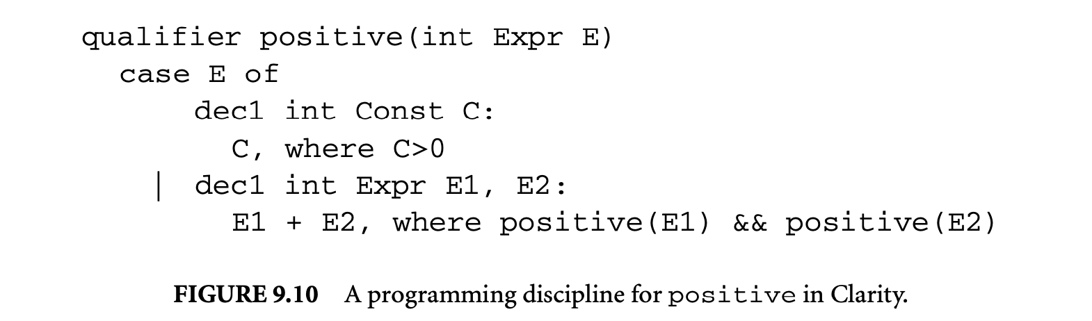 Formally, consider the type system consisting of the rules in Figures 9.8 and 9.9. We remove all the rules of the form , which perform type-checking on constructor expressions, and we remove the annot expression form along with its type-checking rule Q-Annot. When a programmer introduces a new qualifier, he or she must also augment the type system with new inference rules indicating the conditions under which each constructor expression may be given this qualifier. For example, the rules in Figure 9.10 are formally represented by adding the following two rules to the type system:
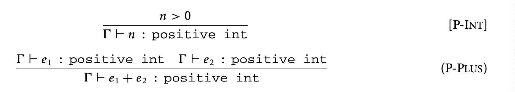
Assuming that the programmer also declares positive nonzero, the subtyping and subsumption rules in Figure 9.9 allow the above rules to be used to give the qualifier nonzero to an expression as well.
Not all qualifiers have natural rules associated with them. For example, the programming disciplines associated with qualifiers such as tainted and untainted could be program dependent and/or quite complicated. Therefore, in practice both the Clarity and CQUAL approaches are useful.
9.3.3.4.1 Type Soundness
A type soundness theorem analogous to that for traditional type qualifiers, which guarantees that asserts succeed at runtime, can be proven in this setting. In addition, it is possible to prove a stronger notion of type soundness. Clarity allows the programmer to optionally specify the set of values associated with a particular qualifier. For example, the programmer could associate the set of positive integers with the positive qualifier. Given this information, type soundness says that a well-typed expression with the qualifier positive will evaluate to a member of the specified set.
To ensure this form of type soundness, Clarity generates one proof obligation per programmer-defined rule. For example, the second rule for positive above requires proving that the sum of two integers greater than zero is also an integer greater than zero. Clarity discharges proof obligations automatically using off-the-shelf decision procedures 38, but in general these may need to be manually proven by the qualifier designer.
This form of type soundness validates the programmer-defined rules. For example, if the second rule for positive above were erroneously defined for subtraction rather than addition, the error would be caught because the associated proof obligation is not valid: the difference between two positive integers is not necessarily positive. In this way, programmers obtain a measure of confidence that their qualifiers and associated inference rules are behaving as intended.
9.3.3.4.2 Qualifier Inference
Qualifier inference is also possible in this setting and is implemented in Clarity, allowing the qualifiers for variables to be inferred rather than declared by the programmer. Similar to qualifier inference in the
Figure 9.10: A programming discipline for positive in Clarity.
previous subsection, a set of subtype constraints is generated and solved. However, handling programmer-defined inference rules requires a form of conditional subtype constraints to be solved 39.
9.3.4 Related Work on Type Refinements
Work on refinement types for the ML language allows programmers to create subtypes of data type definitions 40, each denoting a subset of the values of the data type. For example, a standard list data type could be refined to define a type of nonempty lists. The language for specifying these refinements is analogous to the language for programmer-defined inference rules in Clarity.
Other work has shown how to make refinement types and type qualifiers flow sensitive41, which allows the refinement of an expression to change over time. For example, a file pointer could have the qualifier closed upon creation and the qualifier open after it has been opened. In this way, type refinements can be used to track temporal protocols, for example, that a file must be opened before it can be read or written.
Finally, others have explored type refinements through the notion of dependent types42, in which types can depend on program expressions. An instance of this approach is Dependent ML 43, which allows types to be refined through their dependence on linear arithmetic expressions. For example, the type int list(5) represents integer lists of length 5, and a function that adds an element to an integer list would be declared to have the argument type int list(n) for some integer n and to return a value of type int list(n+1). These kinds of refinements are targeted at qualitatively different kinds of program properties from those targeted by type qualifiers.
References
Jonathan Aldrich, Valentin Kostadinov, and Craig Chambers. 2002. Alias annotations for program understanding. In Proceedings of the 17th ACM SIGPLAN Conference on Object-Oriented Programming, Systems, Languages, and Applications, 311-30. New York: ACM Press. 45: David F. Bacon and Peter F. Sweeney. 1996. Fast static analysis of C++ virtual function calls. SIGPLAN Notices 31(10): 324-41. 46: Anindya Banerjee and David A. Naumann. 2002. Representation independence, confinement and access control. In Proceedings of POPL02, SIGPLAN-SIGACT Symposium on Principles of Programming Languages, 166-77. 47: Mike Barnett, Robert DeLine, Manuel Fahadhrich, K. Rustan M. Leino, and Wolfram Schulte. 2003. Verification of object-oriented programs with invariants. In Fifth Workshop on Formal Techniques for Java-Like Programs. 48: Bruno Blanchet. 1999. Escape analysis for object oriented languages. Application to Java. SIGPLAN Notices 34(10):20-34. 49: Bruno Blanchet. 2003. Escape analysis for Java: Theory and practice. ACM Transactions on Programming Languages and Systems 25(6):713-75. 50: Jeff Bogda and Urs Holzle. 1999. Removing unnecessary synchronization in Java. SIGPLAN Notices 34(10): 35-46. 51: Boris Bokowski and Jan Vitek. 1999. Confined types. In Proceedings of the Fourteenth Annual Conference on Object-Oriented Programming Systems, Languages, and Applications (OOPSLA'99), 82-96. 52: Chandrasekhar Boyapati, Robert Lee, and Martin Rinard. 2002. Ownership types for safe programming: Preventing data races and deadlocks. In Proceedings of the 17th ACM SIGPLAN Conference on Object-Oriented Programming, Systems, Languages, and Applications, 211-30. New York: ACM Press. 53: Chandrasekhar Boyapati, Alexandru Salcinau, William Beebee, and Martin Rinard. 2003. Ownership types for safe region-based memory management in real-time Java. In ACM Conference on Programming Language Design and Implementation, 324-37. 54: John Boyland. 2001. Alias burying: Unique variables without destructive reads. Software Practice and Experience, 31(6):533-53.
Pete Broadwell, Matt Harren, and Naveen Sastry. 2003. Scrash: A system for generating secure crash information. In USENIX Security Symposium. 30: Luca Cardelli. 1988. A semantics of multiple inheritance. Information and Computation 76(2/3): 138-64. 37: Brian Chin, Shane Markstrum, and Todd Millstein. 2005. Semantic type qualifiers. In PLDI '05: Proceedings of the 2005 ACM SIGPLAN Conference on Programming Language Design and Implementation, 85-95. New York: ACM Press. 39: Brian Chin, Shane Markstrum, Todd Millstein, and Jens Palsberg. 2006. Inference of user-defined type qualifiers and qualifier rules. In European Symposium on Programming. 55: David Clarke. 2001. Object ownership and containment. PhD thesis, School of Computer Science and Engineering, University of New South Wales, Sydney, Australia. 56: David G. Clarke, John M. Potter, and James Noble. 1998. Ownership types for flexible alias protection. In Proceedings of the 13th ACM SIGPLAN Conference on Object-Oriented Programming, Systems, Languages, and Applications, 48-64. New York: ACM Press. 18: Dave Clarke, Michael Richmond, and James Noble. 2003. Saving the world from bad beans: Deployment-time confinement checking. In Proceedings of the ACM Conference on Object-Oriented Programming, Systems, Languages, and Applications (OOPSLA), 374-87. 57: David Clarke and Tobias Wrigstad. 2003. External uniqueness. In 10th Workshop on Foundations of Object-Oriented Languages (FOOL). 25: Patrick Cousot and Radhia Cousot. 1977. Abstract interpretation: A unified lattice model for static analysis of programs by construction or approximation of fixpoints. In Fourth ACM Symposium on Principles of Programming Languages, 238-52. 5: Manuvir Das, Sorin Lerner, and Mark Seigle. 2002. Esp: Path-sensitive program verification in polynomial time. In PLDI '02: Proceedings of the ACM SIGPLAN 2002 Conference on Programming Language Design and Implementation, 57-68. New York: ACM Press. 58: J. Dean, D. Grove, and C. Chambers. 1995. Optimization of object-oriented programs using static class hierarchy analysis. In Proceedings of the Ninth European Conference on Object-Oriented Programming (ECOOP'95), ed. W. Olthoff, 77-101. Aarhus, Denmark: Springer-Verlag. 59: Robert DeLine and Manuel Fahndrich. 2001. Enforcing high-level protocols in low-level software. In Proceedings of the ACM SIGPLAN 2001 Conference on Programming Language Design and Implementation, 59-69. New York: ACM Press. 60: Robert DeLine and Manuel Fahndrich. 2004. Typestates for objects. In Proceedings of the 2004 European Conference on Object-Oriented Programming, LNCS 3086. Heidelberg, Germany: Springer-Verlag. 38: David Detlefs, Greg Nelson, and James B. Saxe. 2005. Simplify: A theorem prover for program checking. Journal of the ACM 52(3):365-473. 61: David Detlefs, K. Rustan, M. Leino, and Greg Nelson. 1996. Wrestling with rep exposure. Technical report, Digital Equipment Corporation Systems Research Center. 62: Alain Deutsch. 1995. Semantic models and abstract interpretation techniques for inductive data structures and pointers. In Proceedings of the ACM SIGPLAN Symposium on Partial Evaluation and Semantics-Based Program Manipulation, 226-229. 23: William F. Dowling and Jean H. Gallier. 1984. Linear-time algorithms for testing the satisfiability of propositional horn formulae. Journal of Logic Programming 1(3):267-84. 7: Margaret A. Ellis and Bjarne Stroustrup. 1990. The annotated C++ reference manual. Reading, MA: Addison-Wesley. 4: David Evans. 1996. Static detection of dynamic memory errors. In PLDI '96: Proceedings of the ACM SIGPLAN 1996 Conference on Programming Language Design and Implementation, 44-53. New York: ACM Press. 63: Manuel Fahndrich, K. Rustan, and M. Leino. 2003. Declaring and checking non-null types in an object-oriented language. In Proceedings of the 18th ACM SIGPLAN Conference on Object-Oriented Programming, Systems, Languages, and Applications, 302-12. New York: ACM Press.
Cormac Flanagan and Stephen N. Freund. 2000. Type-based race detection for Java. In Proceedings of the ACM SIGPLAN 2000 Conference on Programming Language Design and Implementation, 219-32. New York: ACM Press. 65: Cormac Flanagan and Shaz Qadeer. 2003. A type and effect system for atomicity. In Proceedings of the ACM SIGPLAN 2003 Conference on Programming Language Design and Implementation, 338-49. New York: ACM Press. 31: Jeffrey S. Foster. 2002. Type qualifiers: Lightweight specifications to improve software quality. PhD dissertation, University of California, Berkeley. 66: Jeffrey S. Foster, Manuel Fahndrich, and Alexander Aiken. 1999. A theory of type qualifiers. In Proceedings of the 1999 ACM SIGPLAN Conference on Programming Language Design and Implementation, 192-203. New York: ACM Press. 32: Jeffrey S. Foster, Robert Johnson, John Kodumal, and Alex Aiken. 2006. Flow-insensitive type qualifiers. ACM Transactions on Programming Languages and Systems 28(6):1035-87. 67: Jeffrey S. Foster, Tachio Terauchi, and Alex Aiken. 2002. Flow-sensitive type qualifiers. In Proceedings of the ACM SIGPLAN 2002 Conference on Programming Language Design and Implementation, 1-12. New York: ACM Press. 40: Tim Freeman and Frank Pfenning. 1991. Refinement types for ML. In PLDI '91: Proceedings of the ACM SIGPLAN 1991 Conference on Programming Language Design and Implementation, 268-77. New York: ACM Press. 8: James Gosling, Bill Joy, and Guy Steele. 1996. The Java language specification. Reading, MA: Addison-Wesley. 68: Dan Grossman, Greg Morrisett, Trevor Jim, Michael Hicks, Yanling Wang, and James Cheney. 2002. Region-based memory management in Cyclone. In Proceedings of the ACM SIGPLAN 2002 Conference on Programming Language Design and Implementation, 282-93. New York: ACM Press. 22: Christian Grothoff, Jens Palsberg, and Jan Vitek. 2001. Encapsulating objects with confined types. In ACM Transactions on Programming Languages and Systems. Proceedings of OOPSLA'01, ACM SIGPLAN Conference on Object-Oriented Programming Systems, Languages and Applications, 241-53 (to appear in 2007). 69: Nevin Heintze. 1995. Control-flow analysis and type systems. In Proceedings of SAS'95, International Static Analysis Symposium, 189-206. Heidelberg, Germany: Springer-Verlag. 19: Atsushi Igarashi, Benjamin C. Pierce, and Philip Wadler. 2001. Featherweight Java: a minimal core calculus for Java and GJ. ACM Transactions on Programming Languages and Systems 23(3):396-450. 34: Rob Johnson and David Wagner. 2004. Finding user/kernel pointer bugs with type inference. In Proceedings of the 13th USENIX Security Symposium, 119-34. 6: Brian W. Kernighan and Dennis M. Ritchie. 1978. The C programming language. New York: Prentice-Hall. 70: Gary A. Kildall. 1973. A unified approach to global program optimization. In Conference Record of the ACM Symposium on Principles of Programming Languages, 194-206. 71: Yitzhak Mandelbaum, David Walker, and Robert Harper. 2003. An effective theory of type refinements. In Proceedings of the Eighth ACM SIGPLAN International Conference on Functional Programming, 213-25. New York: ACM Press. 42: Per Martin-Lof. 1982. Constructive mathematics and computer programming. In Sixth International Congress for Logic, Methodology, and Philosophy of Science, 153-75. Amsterdam: North-Holland. 9: Microsoft. Microsoft Visual C#. [http://msdn.microsoft.com/vscharp]:(http://msdn.microsoft.com/vscharp). 11: Greg Morrisett, Karl Crary, Neal Glew, Dan Grossman, Richard Samuels, Frederick Smith, David Walker, Stephanie Weirich, and Steve Zdancewic. 1999. Talx86: A realistic typed assembly language. Presented at 1999 ACM Workshop on Compiler Support for System Software, May 1999. 10: Greg Morrisett, David Walker, Karl Crary, and Neal Glew. 1998. From system F to typed assembly language. In Proceedings of POPL'98, 25th Annual SIGPLAN-SIGACT Symposium on Principles of Programming Languages, 85-97.
Peter Muller and Arnd Poetzsch-Heffter. 1999. Universes: A type system for controlling representation exposure. In Programming Languages and Fundamentals of Programming, ed. A. Poetzsch-Heffter and J. Meyer. Fernuniversitat Hagen. 73: George C. Necula, Scott McPeak, and Westley Weimer. 2002. CCured: Type-safe retrofitting of legacy code. In Proceedings of the 29th ACM SIGPLAN-SIGACT Symposium on Principles of Programming Languages, 128-39. New York: ACM Press. 74: Peter Orbaek and Jens Palsberg. 1995. Trust in the -calculus. Journal of Functional Programming 7(6):557-91. 75: Jens Palsberg. 1998. Equality-based flow analysis versus recursive types. ACM Transactions on Programming Languages and Systems 20(6):1251-64. 16: Jens Palsberg. 2001. Type-based analysis and applications. In Proceedings of PASTE'01, ACM SIGPLAN/SIGSOFT Workshop on Program Analysis for Software Tools and Engineering, 20-27. 76: Jens Palsberg and Patrick M. O'Keefe. 1995. A type system equivalent to flow analysis. ACM Transactions on Programming Languages and Systems 17(4):576-99. 77: Jens Palsberg and Christina Pavlopoulou. 2001. From polyvariant flow information to intersection and union types. Journal of Functional Programming, 11(3):263-17. 78: Jens Palsberg and Michael I. Schwartzbach. 1991. Object-oriented type inference. In Proceedings of OOPSLA'91, ACM SIGPLAN Sixth Annual Conference on Object-Oriented Programming Systems, Languages and Applications, 146-61. 79: M. S. Paterson and M. N. Wegman. 1978. Linear unification. Journal of Computer and System Sciences 16:158-67. 1: Benjamin C. Pierce. 2002. Types and programming languages. Cambridge MA: MIT Press. 80: K. Rustan, M. Leino, and Peter Muller. 2004. Object invariants in dynamic contexts. In Proceedings of ECOOP'04, 16th European Conference on Object-Oriented Programming, 491-516. 33: Umesh Shankar, Kunal Talwar, Jeffrey S. Foster, and David Wagner. 2001. Detecting format string vulnerabilities with type qualifiers. In Proceedings of the 10th Usenix Security Symposium. 81: Frank Tip and Jens Palsberg. 2000. Scalable propagation-based call graph construction algorithms. In Proceedings of OOPSLA'00, ACM SIGPLAN Conference on Object-Oriented Programming Systems, Languages and Applications, 281-93. 82: Mads Tofte and Jean-Pierre Talpin. 1994. Implementation of the typed call-by-value -calculus using a stack of regions. In Proceedings of the 21st ACM SIGPLAN-SIGACT Symposium on Principles of Programming Languages, 188-201. New York: ACM Press. 83: Mitchell Wand. 1987. A simple algorithm and proof for type inference. Fundamentae Informaticae X:115-22. 84: John Whaley and Monica Lam. 2004. Cloning-based context-sensitive pointer alias analysis using binary decision diagrams. In Proceedings of PLDI'04, ACM SIGPLAN Conference on Programming Language Design and Implementation. 85: Andrew K. Wright and Matthias Felleisen. 1994. A syntactic approach to type soundness. Information and Computation 115(1):38-94. 86: Hongwei Xi and Frank Pfenning. 1998. Eliminating array bound checking through dependent types. In Proceedings of ACM SIGPLAN Conference on Programming Language Design and Implementation, 249-57. 87: Hongwei Xi and Frank Pfenning. 1999. Dependent types in practical programming. In Proceedings of the 26th ACM SIGPLAN Symposium on Principles of Programming Languages, 214-27. 35: Xiaolan Zhang, Antony Edwards, and Trent Jaeger. 2002. Using cqual for static analysis of authorization hook placement. In USENIX Security Symposium, ed. Dan Boneh, 33-48. 21: Tian Zhao, Jens Palsberg, and Jan Vitek. 2006. Type-based confinement. Journal of Functional Programming 16(1):83-128.
Chapter 10 Dynamic Compilation
14.1 Introduction
The term dynamic compilation refers to techniques for runtime generation of executable code. The idea of compiling parts or all the application code while the program is executing challenges our intuition about overheads involved in such an endeavor, yet recently a number of approaches have evolved that effectively manage this challenging task.
The ability to dynamically adapt executing code addresses many of the existing problems with traditional static compilation approaches. One such problem is the difficulty for a static compiler to fully exploit the performance potential of advanced architectures. In the drive for greater performance, today's microprocessors provide capabilities for the compiler to take on a greater role in performance delivery, ranging from predicated and speculative execution (e.g., for the Intel Itanium processor) to various power consumption control models. To exploit these architectural features, the static compiler usually has to rely on profile information about the dynamic execution behavior of a program. However, collecting valid execution profiles ahead of time may not always be feasible or practical. Moreover, the risk of performance degradation that may result from missing or outdated profile information is high.
Current trends in software technology create additional obstacles to static compilation. These are exemplified by the widespread use of object-oriented programming languages and the trend toward shipping software binaries as collections of dynamically linked libraries instead of monolithic binaries. Unfortunately, the increased degree of runtime binding can seriously limit the effectiveness of traditional static compiler optimization, because static compilers operate on the statically bound scope of the program.
Finally, the emerging Internet and mobile communications marketplace creates the need for the compiler to produce portable code that can efficiently execute on a variety of machines. In an environment of networked devices, where code can be downloaded and executed on the fly, static compilation at the target device is usually not an option. However, if static compilers can only be used to generate platform-independent intermediate code, their role as a performance delivery vehicle becomes questionable.
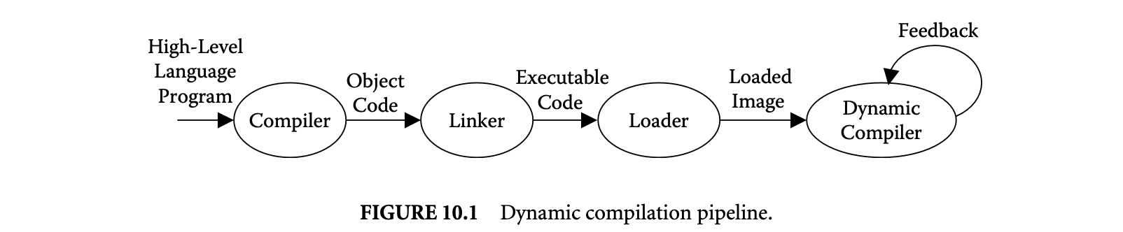
This chapter discusses dynamic compilation, a radically different approach to compilation that addresses and overcomes many of the preceding challenges to effective software implementation. Dynamic compilation extends our traditional notion of compilation and code generation by adding a new dynamic stage to the classical pipeline of compiling, linking, and loading code. The extended dynamic compilation pipeline is depicted in Figure 10.1.
A dynamic compiler can take advantage of runtime information to exploit optimization opportunities not available to a static compiler. For example, it can customize the running program according to information about actual program values or actual control flow. Optimization may be performed across dynamic binding, such as optimization across dynamically linked libraries. Dynamic compilation avoids the limitations of profile-based approaches by directly utilizing runtime information. Furthermore, with a dynamic compiler, the same code region can be optimized multiple times should its execution environment change. Another unique opportunity of dynamic compilation is the potential to speed up the execution of legacy code that was produced using outdated compilation and optimization technology.
Dynamic compilation provides an important vehicle to efficiently implement the "write-once-run-anywhere" execution paradigm that has recently gained a lot of popularity with the Java programming language [22]. In this paradigm, the code image is encoded in a mobile platform-independent format (e.g., Java bytecode). Final code generation that produces native code takes place at runtime as part of the dynamic compilation stage.
In addition to addressing static compilation obstacles, the presence of a dynamic compilation stage can create entirely new opportunities that go beyond code compilation. Dynamic compilation can be used to transparently migrate software from one architecture to a different host architecture. Such a translation is achieved by dynamically retargeting the loaded nonnative guest image to the host machine native format. Even for machines within the same architectural family, a dynamic compiler may be used to upgrade software to exploit additional features of the newer generation.
As indicated in Figure 10.1, the dynamic compilation stage may also include a feedback loop. With such a feedback loop, dynamic information, including the dynamically compiled code itself, may be saved at runtime to be restored and utilized in future runs of the program. For example, the FXl32 system for emulating x86 code on an Alpha platform [27] saves runtime information about executed code, which is then used to produce translations offline that can be incorporated in future runs of the program. It should be noted that FXl32 is not strictly a dynamic compilation system, in that translations are produced between executions of the program instead of online during execution.
Along with its numerous opportunities, dynamic compilation also introduces a unique set of challenges. One such challenge is to amortize the dynamic compilation overhead. If dynamic compilation is sequentially interleaved with program execution, the dynamic compilation time directly contributes to the overall execution time of the program. Such interleaving greatly changes the cost-benefit compilation trade-off that we have grown accustomed to in static compilation. Although in a static compiler increased optimization effort usually results in higher performance, increasing the dynamic compilation time may actually diminish some or all of the performance improvements that were gained by the optimization in the first place. If dynamic compilation takes place in parallel with program execution on a multiprocessor system, the dynamic compilation overhead is less important, because the dynamic compiler cannot directly slow down the program. It does, however, divert resources that could have been devoted to execution. Moreover, long dynamic compilation times can still adversely affect performance. Spending too much time on compilation can delay the employment of the dynamically compiled code and diminish the benefits. To maximize the benefits, dynamic compilation time should therefore always be kept to a minimum.
To address the heightened pressure for minimizing overhead, dynamic compilers often follow an adaptive approach [23]. Initially, the code is optimized with little or no optimization. Aggressive optimizations are considered only later, when more evidence has been found that added optimization effort is likely to be of use.
A dynamic compilation stage, if not designed carefully, can also significantly increase the space requirement for running a program. Controlling additional space requirements is crucial in environments where code size is important, such as embedded or mobile systems. The total space requirements of execution with a dynamic compiler include not only the loaded input image but also the dynamic compiler itself, plus the dynamically compiled code. Thus, care must be taken to control both the footprint of the dynamic compiler and the size of the currently maintained dynamically compiled code.
10.2 Approaches to Dynamic Compilation
A number of approaches to dynamic compilation have been developed. These approaches differ in several aspects, including the degree of transparency, the extent and scope of dynamic compilation, and the assumed encoding format of the loaded image. On the highest level, dynamic compilation systems can be divided into transparent and nontransparent systems. In a transparent system, the remainder of the compilation pipeline is oblivious to the fact that a dynamic compilation stage has been added. The executable produced by the linker and loader is not specially prepared for dynamic optimization, and it may execute with or without a dynamic compilation stage. Figure 10.2 shows a classification of the various approaches to transparent and nontransparent dynamic compilation.
Transparent dynamic compilation systems can further be divided into systems that operate on binary executable code (binary dynamic compilation) and systems that operate on an intermediate platform-independent encoding (just-in-time [JIT] compilation). A binary dynamic compiler starts out with a loaded fully executable binary. In one scenario, the binary dynamic compiler recompiles the binary code to incorporate native-to-native optimizing transformations. These recompilation systems are also referred to as dynamic optimizers[3, 5, 7, 15, 36]. During recompilation, the binary is optimized by customizing the code with respect to specific runtime control and data flow values. In dynamic binary translation, the loaded input binary is in a nonnative format, and dynamic compilation is used to retarget the code to a different host architecture [19, 35, 39]. The dynamic code translation may also include optimization.
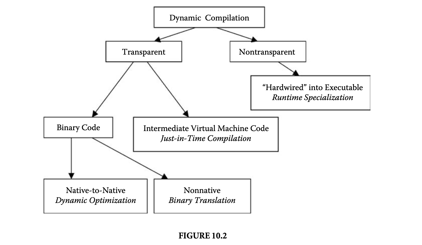
JIT compilers present a different class of transparent dynamic compilers [11, 12, 18, 28, 29]. The input to a JIT compiler is not a native program binary; instead, it is code in an intermediate, platform-independent representation that targets a virtual machine. The JIT compiler serves as an enhancement to the virtual machine to produce native code by compiling the intermediate input program at runtime, instead of executing it in an interpreter. Typically, semantic information is attached to the code, such as symbol tables or constant pools, which facilitates the compilation.
Thealternative to transparent dynamic compilation is the nontransparent approach, which integrates the dynamic compilation stage explicitly within the earlier compilation stages. The static compiler cooperates with the dynamic compiler by delaying certain parts of the compilation to runtime, if their compilation can benefit from runtime values. A dynamic compilation agent is compiled (i.e., hardwired) into the executable to fill and link in a prepared code template for the delayed compilation region. Typically, the programmer indicates adequate candidate regions for dynamic compilation via annotations or compiler directives. Several techniques have been developed to perform runtime specialization of a program in this manner [9, 23, 31, 33].
Runtime specialization techniques are tightly integrated with the static compiler, whereas transparent dynamic compilation techniques are generally independent of the static compiler. However, transparent dynamic compilation can still benefit from information that the static compiler passes down. Semantic information, such as a symbol table, is an example of compiler information that is beneficial for dynamic compilation. If the static compiler is made aware of the dynamic compilation stage, more targeted information may be communicated to the dynamic compiler in the form of code annotations to the binary [30].
The remainder of this chapter discusses the various dynamic compilation approaches shown in Figure 10.2. We first discuss transparent binary dynamic optimization as a representative dynamic compilation system. We discuss the mechanics of dynamic optimization systems and their major components, along with their specific opportunities and challenges. We then discuss systems in each of the remaining dynamic compilation classes and point out their unique characteristics.
Also, a number of hardware approaches are available to dynamically manipulate the code of a running program, such as the hardware in out-of-order superscalar processors or hardware dynamic optimization in trace cache processors [21]. However, in this chapter, we limit the discussion to software dynamic compilation.
10.3 Transparent Binary Dynamic Optimization
A number of binary dynamic compilation systems have been developed that operate as an optional dynamic stage [3, 5, 7, 15, 35]. An important characteristic of these systems is that they take full control of the execution of the program. Recall that in the transparent approach, the input program is not specially prepared for dynamic compilation. Therefore, if the dynamic compiler does not maintain full control over the execution, the program may escape and simply continue executing natively, effectively bypassing dynamic compilation altogether. The dynamic compiler can afford to relinquish control only if it can guarantee that it will regain control later, for example, via a timer interrupt.
Binary dynamic compilation systems share the general architecture shown in Figure 10.3. Input to the dynamic compiler is the loaded application image as produced by the compiler and linker. Two main components of a dynamic compiler are the compiled code cache that holds the dynamically compiled code fragments and the dynamic compilation engine. At any point in time, execution takes place either in the dynamic compilation engine or in the compiled code cache. Correspondingly, the dynamic compilation engine maintains two distinct execution contexts: the context of the dynamic compilation engine itself and the context of the application code.
Execution of the loaded image starts under control of the dynamic compilation engine. The dynamic compiler determines the address of the next instruction to execute. It then consults a lookup table to determine whether a dynamically compiled code fragment starting at that address already exists in the code cache. If so, a context switch is performed to load the application context and to continue execution in the compiled code cache until a code cache miss occurs. A code cache miss indicates that no compiled fragment exists for the next instruction. The cache miss triggers a context switch to reload the dynamic compiler's context and reenter the dynamic compilation engine.
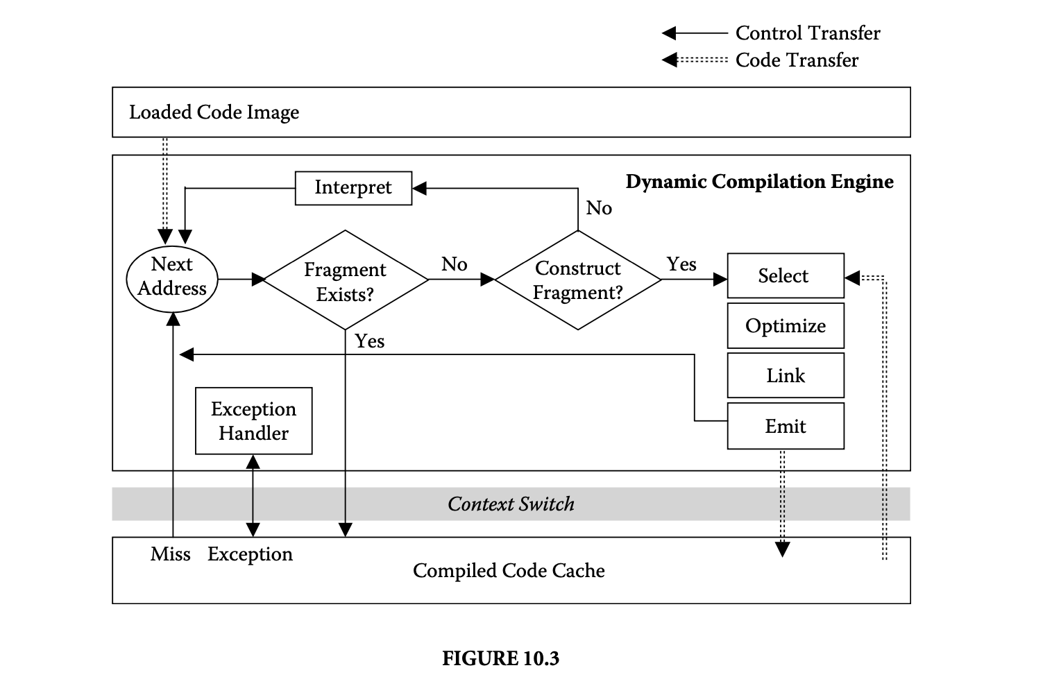 The dynamic compiler decides whether a new fragment should be compiled starting at the next address. If so, a code fragment is constructed based on certain fragment selection policies, which are discussed in the next section. The fragment may optionally be optimized and linked with other previously compiled fragments before it is emitted into the compiled code cache.
The dynamic compilation engine may include an instruction interpreter component. With an interpreter component, the dynamic compiler can choose to delay the compilation of a fragment and instead interpret the code until it has executed a number of times. During interpretation, the dynamic compiler can profile the code to focus its compilation efforts on only the most profitable code fragments [4]. Without an interpreter, every portion of the program that is executed during the current run can be compiled into the compiled code cache.
Figure 10.3 shows a code transfer arrow from the compiled code cache to the fragment selection component. This arrow indicates that the dynamic compiler may choose to select new code fragments from previously created code in the compiled code cache. Such fragment reformation may be performed to improve fragment shape and extent. For example, several existing code fragments may be combined to form a single new fragment. The dynamic compiler may also reselect an existing fragment for more aggressive optimization. Reoptimization of a fragment may be indicated if profiling of the compiled code reveals that it is a hot (i.e., frequently executing) fragment.
In the following sections, we discuss the major components of the dynamic compiler in detail: fragment selection, fragment optimization, fragment linking, management of the compiled code cache, and exception handling.
10.3.1 Fragment Selection
The fragment selector proceeds by extracting code regions and passing them to the fragment optimizer for optimization and eventual placement in the compiled code cache. The arrangement of the extracted code regions in the compiled code cache leads to a new code layout, which has the potential of improving the performance of dynamically compiled code. Furthermore, by passing isolated code regions to the optimizer, the fragment selector dictates the scope and kind of runtime optimization that may be performed. Thus, the goal of fragment selection is twofold: to produce an improved code layout and to expose dynamic optimization opportunities.
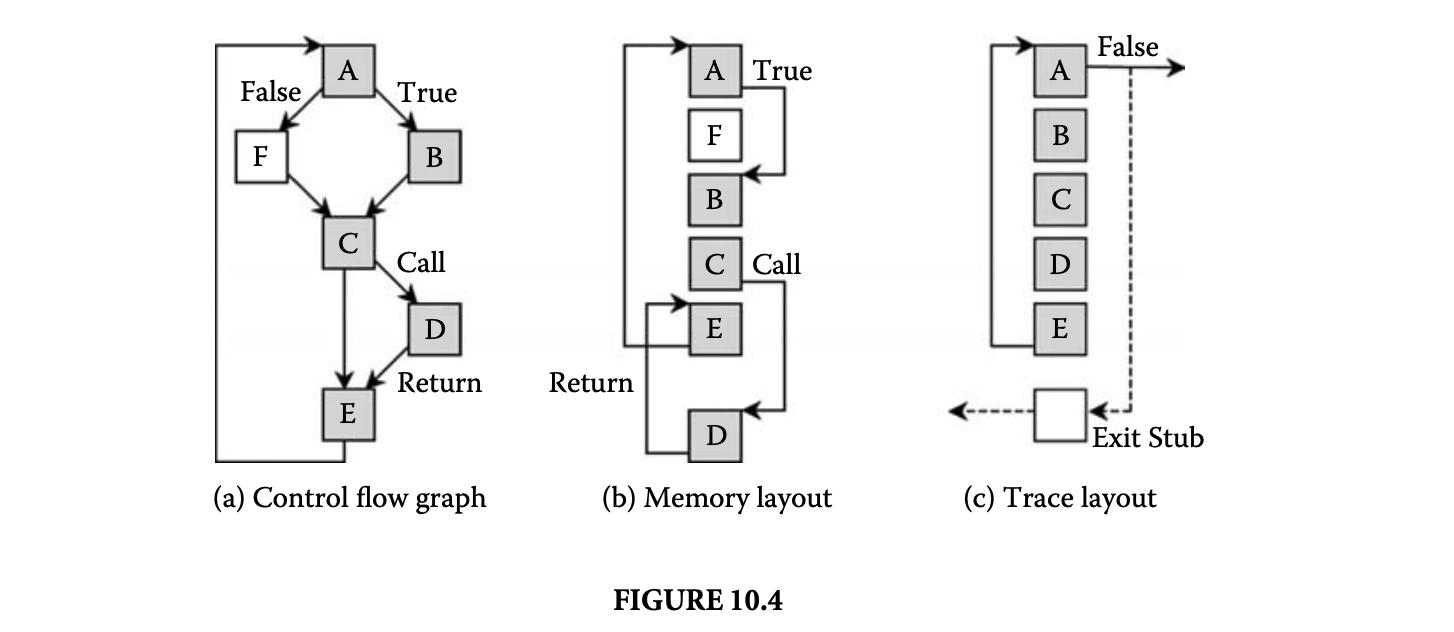 New optimization opportunities or improvements in code layout are unlikely if the fragment selector merely copies static regions from the loaded image into the code cache. Regions such as basic blocks or entire procedures are among the static regions of the original program and have been already exposed to, and possibly optimized by, the static compiler. New optimization opportunities are more likely to be found in the dynamic scope of the executing program. Thus, it is crucial to incorporate dynamic control flow into the selected code regions.
Because of the availability of dynamic information, the fragment selector has an advantage over a static compiler in selecting the most beneficial regions to optimize. At the same time, the fragment selector is more limited because high-level semantic information about code constructs is no longer available. For example, without information about procedure boundaries and the layout of switch statements, it is generally impossible to discover the complete control flow of a procedure body in a loaded binary image.
In the presence of these limitations, the units of code commonly used in a binary dynamic compilation system are a partial execution trace, or trace for short BD [4, 7]. A trace is a dynamic sequence of consecutively executing basic blocks. The sequence may not be contiguous in memory; it may even be interprocedural, spanning several procedure boundaries, including dynamically linked modules. Thus, traces are likely to offer opportunities for improved code layout and optimization. Furthermore, traces do not need to be computed; they can be inferred simply by observing the runtime behavior of the program.
Figure 10.4 illustrates the effects of selecting dynamic execution traces. The graph in Figure 10.4a shows a control flow graph representation of a trace, consisting of blocks A, B, C, D, and E that form a loop containing a procedure call. The graph in Figure 10.4b shows the same trace in a possible noncontiguous memory layout of the original loaded program image. The graph in Figure 10.4c shows a possible improved layout of the looping trace in the compiled code cache as a contiguous straight-line sequence of blocks. The straight-line layout reduces branching during execution and offers better code locality for the loop.
10.3.1.1 Adaptive Fragment Selection
The dynamic compiler may select fragments of varying shapes. It may also stage the fragment selection in a progressive fashion. For example, the fragment selector may initially select only basic block fragments. Larger composite fragments, such as traces, are selected as secondary fragments by stringing together frequently executing block fragments [4]. Progressively larger regions, such as tree regions, may then be constructed by combining individual traces [19]. Building composite code regions can result in potentially large amounts of code duplication because code that is common across several composite regionsis replicated in each region. Uncontrolled code duplication can quickly result in excessive cache size requirements, the so-called code explosion problem. Thus, a dynamic compiler has to employ some form of execution profiling to limit composite region construction to only the (potentially) most profitable candidates.
10.3.1.2 Online Profiling
Profiling the execution behavior of the loaded code image to identify the most frequently executing regions is an integral part of dynamic compilation. Information about the hot spots in the code is used in fragment selection and for managing the compiled code cache space. Hot spots must be detected online as they are becoming hot, which is in contrast to conventional profiling techniques that operate offline and do not establish relative execution frequencies until after execution. Furthermore, to be of use in a dynamic compiler, the profiling techniques must have very low space and time overheads.
A number of offline profiling techniques have been developed for use in feedback systems, such as profile-based optimization. A separate profile run of the program is conducted to accumulate profile information that is then fed back to the compiler. Two major approaches to offline profiling are statistical PC sampling and binary instrumentation for the purpose of branch or path profiling. Statistical PC sampling [1, 10, 40] is an inexpensive technique for identifying hot code blocks by recording program counter hits. Although PC sampling is efficient for detecting individual hot blocks, it provides little help in finding larger hot code regions. One could construct a hot trace by stringing together the hottest code blocks. However, such a trace may never execute from start to finish because the individual blocks may have been hot along disjoint execution paths. The problem is that individually collected branch frequencies do not account for branch correlations, which occur if the outcome of one branch can influence the outcome of a subsequent branch.
Another problem with statistical PC sampling is that it introduces nondeterminism into the dynamic compilation process. Nondeterministic behavior is undesirable because it greatly complicates development and debugging of the dynamic compiler.
Profiling techniques based on binary instrumentation record information at every execution instance. They are more costly than statistical sampling, but can also provide more fine-grained frequency information. Like statistical sampling, branch profiling techniques suffer the same problem of not adequately addressing branch correlations. Path-profiling techniques overcome the correlation problem by directly determining hot traces in the program [6]. The program binary is instrumented to collect entire path (i.e., trace) frequency information at runtime in an efficient manner.
A dynamic compiler could adopt these techniques by inserting instrumentation in first-level code fragments to build larger composite secondary fragments. The drawback of adapting offline techniques is the large amount of profile information that is collected and the overhead required to process it. Existing dynamic compilation systems have employed more efficient, but also more approximate, profiling schemes that collect a small amount of profiling information, either during interpretation [5] or by instrumenting first-level fragments [19]. Ephemeral instrumentation is a hybrid profiling technique [37] based on the ability to efficiently enable and disable instrumentation code.
10.3.1.3 Online Profiling in the Dynamo System
As an example of a profiling scheme used in a dynamic compiler, we consider the next executing tail (NET) scheme used in the Dynamo system [16]. The objective of the NET scheme is to significantly reduce profiling overhead while still providing effective hot path predictions. A path is divided into a path head (i.e., the path starting point) and a path tail, which is the remainder of the path following the starting point. For example, in path ABCDE in Figure 10.4a, block A is the path head and BCDE is the path tail. The NET scheme reduces profiling cost by using speculation to predict path tails, while maintaining full profiling support to predict hot path heads. The rationale behind this scheme is that a hot path head indicates that the program is currently executing in a hot region, and the next executing path tail is likely to be part of that region.
Accordingly, execution counts are maintained only for potential path heads, which are the targets of backward taken branches or the targets of cache exiting branches. For example, in Figure 10.4a, one profiling count is maintained for the entire loop at the single path head at the start of block A. Once the counter at block A has exceeded a certain threshold, the next executing path is selected as the hot path for the loop.
10.3.2 Fragment Optimization
After a fragment has been selected, it is translated into a self-contained location-independent intermediate representation (IR). The IR of a fragment serves as a temporary vehicle to transform the original instruction stream into an optimized form and to prepare it for placement and layout in the compiled code cache. To enable fast translation between the binary code and the IR, the abstraction level of the IR is kept close to the binary instruction level. Abstraction is introduced only when needed, such as to provide location independence through symbolic labels and to facilitate code motion and code transformations through the use of virtual registers.
After the fragment is translated into its intermediate form, it can be passed to the optimizer. A dynamic optimizer is not intended to duplicate or replace conventional static compiler optimization. On the contrary, a dynamic optimizer can complement a static compiler by exploiting optimization opportunities that present themselves only at runtime, such as value-based optimization or optimization across the boundaries of dynamically linked libraries. The dynamic optimizer can also apply path-specific optimization that would be too expensive to apply indiscriminately over all paths during static compilation. On a given path, any number of standard compiler optimizations may be performed, such as constant and copy propagation, dead code elimination, value numbering, and redundancy elimination [4, 15]. However, unlike in static compiler optimization, the optimization algorithm must be optimized for efficiency instead of generality and power. A traditional static optimizer performs an initial analysis phase over the code to collect all necessary data flow information that is followed by the actual optimization phase. The cost of performing multiple passes over the code is likely to be prohibitive in a runtime setting. Thus, a dynamic optimizer typically combines analysis and optimization into a single pass over the code [4]. During the combined pass all necessary data flow information is gathered on demand and discarded immediately if it is no longer relevant for current optimization [17].
10.3.2.1 Control Specialization
The dynamic compiler implicitly performs a form of control specialization of the code by producing a new layout of the running program inside the compiled code cache. Control specialization describes optimizations whose benefits are based on the execution taking specific control paths. Another example of control specialization is code sinking [4], also referred to as hot-cold optimization [13]. The objective of code sinking is to move instructions from the main fragment execution path into fragment exits to reduce the number of instructions executed on the path. An instruction can be sunk into a fragment exit block if it is not live within the fragment. Although an instruction appears dead on the fragment, it cannot be removed entirely because it is not known whether it is also dead after exiting the fragment.
An example of code sinking is illustrated in Figure 10.5. The assignment X: = Y in the first block in fragment 1 is not live within fragment 1 because it is overwritten by the read instruction in the next block. To avoid useless execution of the assignment when control remains within fragment 1, the assignment can be moved out of the fragment and into a so-called compensation block at every fragment exit at which the assigned variable may still be live, as shown in Figure 10.5. Once the exit block is linked to a target fragment (fragment 2 in Figure 10.5) the code inside the target fragment can be inspected to determine whether the moved assignment becomes dead after linking. If it does, the moved assignment in the compensation block can safely be removed, as shown in Figure 10.5.
Another optimization is prefetching, which involves the placement of prefetch instructions along execution paths prior to the actual usage of the respective data to improve the memory behavior of the dynamically compiled code. If the dynamic compiler can monitor data cache latency, it can easily identify candidates for prefetching. A suitable placement of the corresponding prefetch instructions can be determined by consulting collected profile information.
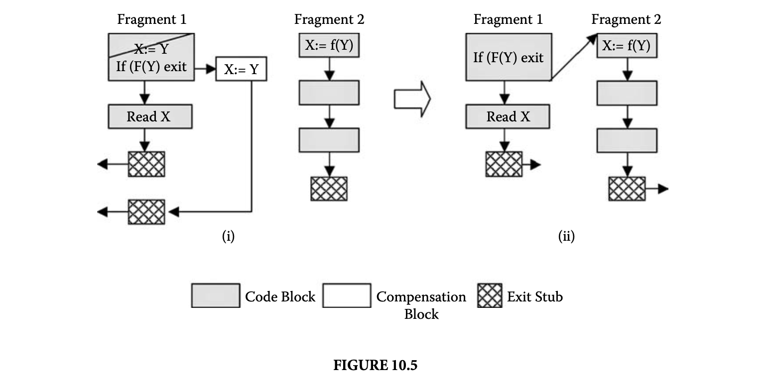
10.3.2.2 Value Specialization
Value specialization refers to an optimization that customizes the code according to specific runtime values of selected specialization variables. The specialization of a code fragment proceeds like a general form of constant propagation and attempts to simplify the code as much as possible.
Unless it can be established for certain that the specialization variable is always constant, the execution of the specialized code must be guarded by a runtime test. To handle specialization variables that take on multiple values at runtime, the same region of code may be specialized multiple times. Several techniques, such as polymorphic in-line caches [25], have been developed to efficiently select among multiple specialization versions at runtime.
A number of runtime techniques have been developed that automatically specialize code at runtime, given a specification of the specialization variables [9, 23, 31]. In code generated from object-oriented languages, virtual method calls can be specialized for a common receiver class [25]. In principle, any code region can be specialized with respect to any number of values. For example, traces may be specialized according to the entry values of certain registers. In the most extreme case, one can specialize individual instructions, such as complex floating point instructions, with respect to selected fixed-input register values [34].
The major challenge in value specialization is to decide when and what to specialize. Overspecialization of the code can quickly result in code explosion and may severely degrade performance. In techniques that specialize entire functions, the programmer typically indicates the functions to specialize through code annotations prior to execution [9, 23]. Once the specialization regions are determined, the dynamic specializer monitors the respective register values at runtime to trigger the specialization. Runtime specialization is the primary optimization technique employed by nontransparent dynamic compilation systems. We revisit runtime specialization in the context of nontransparent dynamic compilation in Section 10.6.
10.3.2.3 Binary Optimization
The tasks of code optimization and transformation are complicated by having to operate on executable binary code instead of a higher-level intermediate format. The input code to the dynamic optimizer has previously been exposed to register allocation and possibly also to static optimization. Valuable semantic information that is usually incorporated into compilation and optimization, such as type information and information about high-level constructs (i.e., data structures), is no longer available and is generally difficult to reconstruct.
An example of an optimization that is relatively easy to perform on intermediate code but difficult on the binary level is procedure inlining. To completely inline a procedure body, the dynamic compiler has toreverse engineer the implemented calling convention and stack frame layout. Doing this may be difficult, if not impossible, in the presence of memory references that cannot be disambiguated from stack frame references. Thus, the dynamic optimizer may not be able to recognize and entirely eliminate instructions for stack frame allocation and deallocation or instructions that implement caller and callee register saves and restores.
The limitations that result from operating on binary code can be partially lifted by making certain assumptions about compiler conventions. For example, assumptions about certain calling or register usage conventions help in the procedure inlining problem. Also, if it can be assumed that the stack is only accessed via a dedicated stack pointer register, stack references can be disambiguated from other memory references. Enhanced memory disambiguation may then in turn enable more aggressive optimization.
10.3.3 Fragment Linking
Fragment linking is the mechanism by which control is transferred among fragments without exiting the compiled code cache. An important performance benefit of linking is the elimination of unnecessary context switches that are needed to exit and reenter the code cache.
The fragment-linking mechanism may be implemented via exit stubs that are initially inserted at every fragment exiting branch, as illustrated in Figure 10.6. Prior to linking, the exit stubs direct control to the context switch routine to transfer control back to the dynamic compilation engine. If a target fragment for the original exit branch already exists in the code cache, the dynamic compiler can patch the exiting branch to jump directly to its target inside the cache. For example, in Figure 10.6, the branches A to E and G to A have been directly linked, leaving their original exit stubs inactive. To patch exiting branches, some information about the branch must be communicated to the dynamic compiler. For example, to determine the target fragment of a link, the dynamic compiler must know the original target address of the exiting branch. This kind of branch information may be stored in a link record data structure, and a pointer to it can be embedded in the exit stub associated with the branch [4].
The linking of an indirect computed branch is more complicated. If the fragment selector has collected a preferred target for the indirect branch, it can be inlined directly into the fragment code. The indirect target is inlined by converting the indirect branch into a conditional branch that tests whether the current target is equal to the preferred target. If the test succeeds, control falls through to the preferred target inside the fragment. Otherwise, control can be directed to a special lookup routine that is permanently resident in the compiled code cache. This routine implements a lookup to determine whether a fragment for the indirect branch target is currently resident in the cache. If so, control can be directed to the target fragment without having to exit the code cache [4].
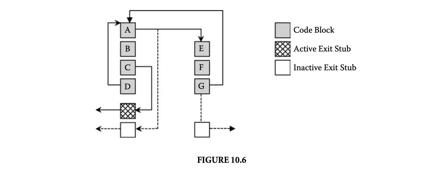 Although its advantages are obvious, linking also has some disadvantages that need to be kept in balance when designing the linker. For example, linking complicates the effective management of the code cache,which may require the periodic removal or relocation of individual fragments. The removal of a fragment may be necessary to make room for new fragments, and fragment relocation may be needed to periodically defragment the code cache. Linking complicates both the removal and relocation of individual fragments because all incoming fragment links have to be unlinked first. Another problem with linking is that it makes it more difficult to limit the latency of asynchronous exception handling. Asynchronous exceptions arise from events such as keyboard interrupts and timer expiration. Exception handling is discussed in more detail in Section 10.3.5.
Linking may be performed on either a demand basis or a preemptive basis. With on-demand linking, fragments are initially placed in the cache with all their exiting branches targeting an exit stub. Individual links are inserted as needed each time control exits the compiled code cache via an exit stub. With preemptive linking, all possible links are established when a fragment is first placed in the code cache. Preemptive linking may result in unnecessary work when links are introduced that are never executed. On the other hand, demand-based linking causes additional context switches and interruptions of cache execution each time a delayed link is established.
10.3.4 Code Cache Management
The code cache holds the dynamically compiled code and may be organized as one large contiguous area of memory, or it may be divided into a set of smaller partitions. Managing the cache space is a crucial task in the dynamic compilation system. Space consumption is primarily controlled by a cache allocation and deallocation strategy. However, it can also be influenced by the fragment selection strategy. Cache space requirements increase with the amount of code duplication among the fragments. In the most conservative case, the dynamic compiler selects only basic block fragments, which avoids code duplication altogether. However, the code quality and layout in the cache is likely to be unimproved over the original binary. A dynamic compiler may use an adaptive strategy that permits unlimited duplication if sufficient space is available but moves toward shorter, more conservatively selected fragments as the available space in the cache diminishes. Even with an adaptive strategy, the cache may eventually run out of space, and the deallocation of code fragments may be necessary to make room for future fragments.
10.3.4.1 Fragment Deallocation
A fragment deallocation strategy is characterized by three parameters: the granularity, the timing, and the replacement policy that triggers deallocation. The granularity of fragment deallocation may range from an individual fragment deallocation to an entire cache flush. Various performance tradeoffs are to be considered in choosing the deallocation granularity. Individual fragment deallocation is costly in the presence of linking because each fragment exit and entry has to be individually unlinked. To reduce the frequency of cache management events, one might choose to deallocate a group of fragments at a time. A complete flush of one of the cache partitions is considerably cheaper because individual exit and entry links do not have to be processed. Moreover, complete flushing does not incur fragmentation problems. However, uncontrolled flushing may result in loss of useful code fragments that may be costly to reacquire.
The timing of a deallocation can be demand or preemptive based. A demand-based deallocation occurs simply in reaction to an out-of-space condition of the cache space. A preemptive strategy is used in the Dynamo system for cache flushing [4]. The idea is to time a cache flush so that the likelihood of losing valuable cache contents is minimized. The Dynamo system triggers a cache flush when it detects a phase change in the program behavior. When a new program phase is entered, a new working set of fragments is built, and it is likely that most of the previously active code fragments are no longer relevant. Dynamo predicts phase changes by monitoring the fragment creation rate. A phase change is signaled if a sudden increase in the creation rate is detected.
Finally, the cache manager has to implement a replacement policy. A replacement policy is particularly important if individual fragments are deallocated. However, even if an entire cache partition is flushed, a decision has to be made as to which partition to free. The cache manager can borrow simple common replacement policies from memory paging systems, such as first-in, first-out (FIFO) or least recently used (LRU). Alternatively, more advanced garbage collection strategies, such as generational garbage collection strategies, can be adopted to manage the dynamic compilation cache.
Besides space allocation and deallocation, an important code cache service is the fast lookup of fragments that are currently resident in the code cache. Fragment lookups are needed throughout the dynamic compilation system and even during the execution of cached code fragments when it is necessary to look up an indirect branch target. Thus, fast implementation of fragment lookups, for example, via hash tables, is crucial.
10.3.4.2 Multiple Threads
The presence of multithreading can greatly complicate the cache manager. Most of the complication from multithreading can simply be avoided by using thread-private caches. With thread-private caches, each thread uses its own compiled code cache, and no dynamically compiled code is shared among threads. However, the lack of code sharing with thread-private caches has several disadvantages. The total code cache size requirements are increased by the need to replicate thread-shared code in each private cache. Besides additional space requirements, the lack of code sharing can also cause redundant work to be carried out when the same thread-shared code is repeatedly compiled.
To implement shared code caches, every code cache access that deletes or adds fragment code must be synchronized. Operating systems usually provide support for thread synchronization. To what extent threads actually share code and, correspondingly, to what extent shared code caches are beneficial are highly dependent on the application behavior.
Another requirement for handling multiple threads is the provision of thread-private state. Storage for thread-private state is needed for various tasks in the dynamic compiler. For example, during fragment selection a buffer is needed to hold the currently collected fragment code. This buffer must be thread private to avoid corrupting the fragment because multiple threads may be simultaneously in the process of creating fragments.
10.3.5 Handling Exceptions
The occurrence of exceptions while executing in the compiled code cache creates a difficult issue for a dynamic compiler. This is true for both user-level exceptions, such as those defined in the Java language, and system-level exceptions, such as memory faults. An exception has to be serviced as if the original program is executing natively. To ensure proper exception handling, the dynamic compiler has to intercept all exceptions delivered to the program. Otherwise, the appropriate exception handler may be directly invoked, and the dynamic compiler may lose control over the program. Losing control implies that the program has escaped and can run natively for the remainder of the execution.
The original program may have installed an exception handler that examines or even modifies the execution state passed to it. In binary dynamic compilation, the execution state includes the contents of machine registers and the program counter. In JIT compilation, the execution state depends on the underlying virtual machine. For example, in Java, the execution state includes the contents of the Java runtime stack.
If an exception is raised when control is inside the compiled code cache, the execution state may not correspond to any valid state in the original program. The exception handler may fail or operate inadequately when an execution state has been passed to it that was in some way modified through dynamic compilation. The situation is further complicated if the dynamic compiler has performed optimizations on the dynamically compiled code.
Exceptions can be classified as asynchronous or synchronous. Synchronous exceptions are associated with a specific faulting instruction and must be handled immediately before execution can proceed. Examples of synchronous exceptions are memory or hardware faults. Asynchronous exceptions do not require immediate handling, and their processing can be delayed. Examples of asynchronous exceptions include external interrupts (e.g., keyboard interrupts) and timer expiration.
A dynamic compiler can deal with asynchronous exceptions by delaying their handling until a safe execution point is reached. A safe point describes a state at which the precise execution state of the original program is known. In the absence of dynamic code optimization, a safe point is usually reached when control is inside the dynamic compilation engine. When control exits the code cache, the original execution state is saved by the context switch routine prior to reentering the dynamic compilation engine. Thus, the saved context state can be restored before executing the exception handler.
If control resides inside the code cache at the time of the exception, the dynamic compiler can delay handling the exception until the next code cache exit. Because the handling of the exception must not be delayed indefinitely, the dynamic compiler may have to force a code cache exit. To force a cache exit, the fragment that has control at the time of the exception is identified, and all its exit branches are unlinked. Unlinking the exit branches prevents control from spinning within the code cache for an arbitrarily long period of time before the dynamic compiler can process the pending exception.
10.3.5.1 Deoptimization
Unfortunately, postponing the handling of an exception until a safe point is reached is not an option for synchronous exceptions. Synchronous exceptions must be handled immediately, even if control is at a point in the compiled code cache. The original execution state must be recovered as if the original program had executed unmodified. Thus, at the very least, the program counter address, currently a cache address, has to be set to its corresponding address in the original code image.
The situation is more complicated if the dynamic compiler has applied optimizations that change the execution state. This includes optimizations that eliminate code, remap registers, or reorder instructions. In Java JIT compilation, this also includes the promotion of Java stack locations to machine registers. To reestablish the original execution state, the fragment code has to be deoptimized. This problem of deoptimization is similar to one that arises with debugging optimized code, where the original unoptimized user state has to be presented to the programmer when a break point is reached.
Deoptimization techniques for runtime compilation have previously been discussed for JIT compilation [26] and binary translation [24]. Each optimization requires its own deoptimization strategy, and not all optimizations are deoptimizable. For example, the reordering of two memory load operations cannot be undone once the reordered earlier load has executed and raised an exception. To deoptimize a transformation, such as dead code elimination, several approaches can be followed. The dynamic compiler can store sufficient information at every optimization point in the dynamically compiled code. When an exception arises, the stored information is consulted to determine the compensation code that is needed to undo the optimization and reproduce the original execution state. For dead code elimination, the compensation code may be as simple as executing the eliminated instruction. Although this approach enables fast state recovery at exception time, it can require substantial storage for deoptimization information.
An alternative approach, which is better suited if exceptions are rare events, is to retrieve the necessary deoptimization information by recompiling the fragment at exception time. During the initial dynamic compilation of a fragment, no deoptimization information is stored. This information is recorded only during a recompilation that takes place in response to an exception.
It may not always be feasible to determine and store appropriate deoptimization information, for example, for optimizations that exploit specific register values. To be exception-safe and to faithfully reproduce original program behavior, a dynamic compiler may have to suppress optimizations that cannot be deoptimized if an exception were to arise.
10.3.6 Challenges
The previous sections have discussed some of the challenges in designing a dynamic optimization system. A number of other difficult issues still must be dealt with in specific scenarios.
10.3.6.1 Self-Modifying and Self-Referential Code
One such issue is the presence of self-modifying or self-referential code. For example, self-referential code may be inserted for a program to compute a check sum on its binary image. To ensure that self-referential behavior is preserved, the loaded program image should remain untouched, which is the case if the dynamic compiler follows the design illustrated in Figure 10.3.
Self-modifying code is more difficult to handle properly. The major difficulty lies in the detection of code modification. Once code modification has been detected, the proper reaction is to invalidate all fragments currently resident in the cache that contain copies of the modified code. Architectural support can make the detection of self-modifying code easy. If the underlying machine architecture provides page-write protection, the pages that hold the loaded program image can simply be write protected. A page protection violation can then indicate the occurrence of code modification and can trigger the corresponding fragment invalidations in the compiled code cache. Without such architectural support, every store to memory must be intercepted to test for self-modifying stores.
10.3.6.2 Transparency
A truly transparent dynamic compilation system can handle any loaded executable. Thus, to qualify as transparent a dynamic compiler must not assume special preparation of the binary, such as explicit relinking or recompilation with dynamic compilation code. To operate fully transparently, a dynamic compiler should be able to handle even legacy code. In a more restrictive setting, a dynamic compiler may be allowed to make certain assumptions about the loaded code. For example, an assumption may be made that the loaded program was generated by a compiler that obeys certain software conventions. Another assumption could be that it is equipped with symbol table information or stack unwinding information, each of which may provide additional insights into the code that can be valuable during optimization.
10.3.6.3 Reliability
Reliability and robustness present another set of challenges. If the dynamic compiler acts as an optional transparent runtime stage, robust operation is of even greater importance than in static compilation stages. Ideally, the dynamic compilation system should reach hardware levels of robustness, though it is not clear how this can be achieved with a piece of software.
10.3.6.4 Real-Time Constraints
Handling real-time constraints in a dynamic compiler has not been sufficiently studied. The execution speed of a program that runs under the control of a dynamic compiler may experience large variations. Initially, when the code cache is nearly empty, dynamic compilation overhead is high and execution progress is correspondingly slow. Over time, as a program working set materializes in the code cache, the dynamic compilation overhead diminishes and execution speed picks up. In general, performance progress is highly unpredictable because it depends on the code reuse rate of the program. Thus, it is not clear how any kind of real-time guarantees can be provided if the program is dynamically compiled.
10.4 Dynamic Binary Translation
The previous sections have described dynamic compilation in the context of code transformation for performance optimization. Another motivation for employing a dynamic compiler is software migration. In this case, the loaded image is native to a guest architecture that is different from the host architecture, which runs the dynamic compiler. The binary translation model of dynamic compilation is illustrated in Figure 10.7. Caching instruction set simulators [8] and dynamic binary translation systems [19, 35, 39] are examples of systems that use dynamic compilation to translate nonnative guest code to a native host architecture.
An interesting aspect of dynamic binary translation is achieving separation of the running software from the underlying hardware. In principle, a dynamic compiler can provide a software implementationof an arbitrary guest architecture. With the dynamic compilation layer acting as a bridge, software and hardware may evolve independently. Architectural advances can be hidden and remain transparent to the user. This potential of dynamic binary translation has recently been commercially exploited by Transmeta's code morphing software [14] and Transitive's emulation software layer [38].
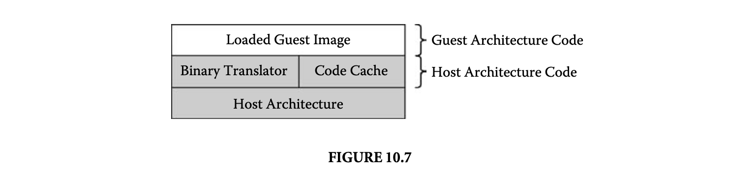
The high-level design of a dynamic compiler, if used for binary translation, remains the same as illustrated in Figure 10.3, with the addition of a translation module. This additional module translates fragments selected from guest architecture code into fragments for the host architecture, as illustrated in Figure 10.8.
To produce a translation from one native code format to another, the dynamic compiler may choose to first translate the guest architecture code into an intermediate format and then generate the final host architecture instructions. Going through an intermediate format is especially helpful if the differences in host and guest architecture are large. To facilitate the translation of instructions, it is useful to establish a fixed mapping between guest and host architecture resources, such as machine registers [19].
Although the functionality of the major components in the dynamic compilation stage, such as fragment selection and code cache management, is similar to the case of native dynamic optimization, a number of important challenges are unique to binary translation.
If the binary translation system translates code not only across different architectures but also across different operating systems, it is called full system translation. The Daisy binary translation system that translates from code for the PowerPC under IBM's UNIX system, AIX, to a customized very long instruction word (VLIW) architecture is an example of full system translation [19]. Full system translation may be further complicated by the presence of a virtual address space in the guest system. The entire virtual memory address translation mechanism has to be faithfully emulated during the translation, which includes the handling of such events as page faults. Furthermore, low-level boot code sequences must also be translated. Building a dynamic compiler for full system translation requires in-depth knowledge of both the guest and host architectures and operating systems.
10.5 Just-in-Time Compilation
JIT compilation refers to the runtime compilation of intermediate virtual machine code. Thus, unlike binary dynamic compilation, the process does not start out with already compiled executable code. JIT compilation was introduced for Smalltalk-80 [18] but has recently been widely popularized with the introduction of the Java programming language and its intermediate bytecode format [22].
The virtual machine environment for a loaded intermediate program is illustrated in Figure 10.9. As in binary dynamic compilation, the virtual machine includes a compilation module and a compiled code cache. Another core component of the virtual machine is the runtime system that provides various system services that are needed for the execution of the code.
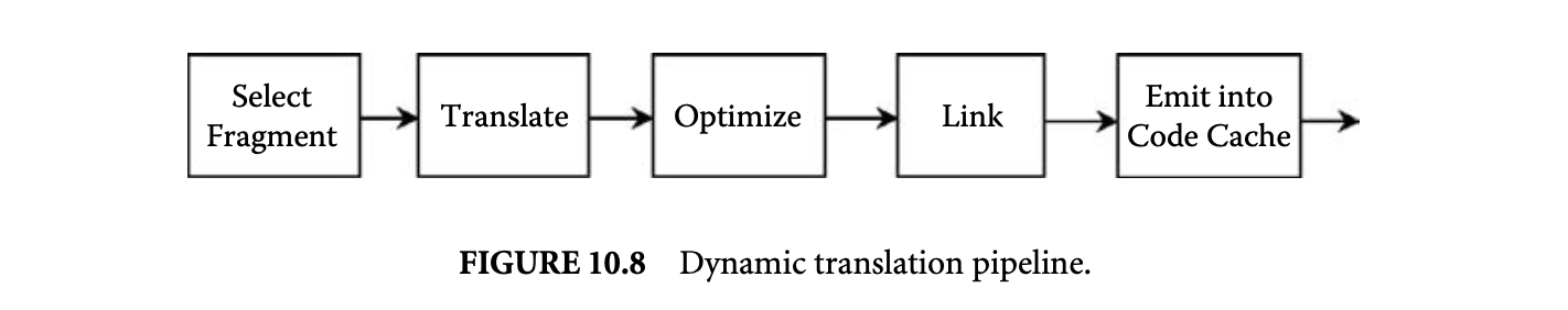

The loaded intermediate code image is inherently tied to, and does not execute outside, the virtual machine. Virtual machines are an attractive model to implement a "write-once-run-anywhere" programming paradigm. The program is statically compiled to the virtual machine language. In principle, the same statically compiled program may run on any hardware environment, as long as the environment provides an appropriate virtual machine. During execution in the virtual machine, the program may be further (JIT) compiled to the particular underlying machine architecture. A virtual machine with a JIT compiler may or may not include a virtual machine language interpreter.
JIT compilation and binary dynamic compilation share a number of important characteristics. In both cases, the management of the compiled code cache is crucial. Just like a binary dynamic compiler, the JIT compiler may employ profiling to stage the compilation and optimization effort into several modes, from a quick base compilation mode with no optimization to an aggressively optimized mode.
Some important differences between JIT and binary dynamic compilation are due to the different levels of abstraction in their input. To facilitate execution in the virtual machine, the intermediate code is typically equipped with semantic information, such as symbol tables or constant pools. A JIT compiler can take advantage of the available semantic information. Thus, JIT compilation more closely resembles the process of static compilation than does binary recompilation.
The virtual machine code that the JIT compiler operates on is typically location independent, and information about program components, such as procedures or methods, is available. In contrast, binary dynamic compilers operate on fully linked binary code and usually face a code recovery problem. To recognize control flow, code layout decisions that were made when producing the binary have to be reverse engineered, and full code recovery is in general not possible. Because of the code recovery problem, binary dynamic compilers are more limited in their choice of compilation unit. They typically choose simple code units, such as straight-line code blocks, traces, or tree-shaped regions. JIT compilers, on the other hand, can recognize higher-level code constructs and global control flow. They typically choose whole methods or procedures as the compilation unit, just as a static compiler would do. However, recently it has been recognized that there are other advantages to considering compilation units at a different granularity than whole procedures, such as reduced compiled code sizes [2].
The availability of semantic information in a JIT compiler also allows for a larger optimization repertoire. Except for overhead concerns, a JIT compiler is just as capable of optimizing the code as a static compiler. JIT compilers can even go beyond the capabilities of a static compiler by taking advantage of dynamic information about the code. In contrast, a binary dynamic optimizer is more constrained by the low-level representation and the lack of a global view of the program. The aliasing problem is worse in binary dynamic compilation because the higher-level-type information that may help disambiguate memory references is not available. Furthermore, the lack of a global view of the program forces the binary dynamic compiler to make worst-case assumptions at entry and exit points of the currently processed code fragment, which may preclude otherwise safe optimizations.
 The differences in JIT compilation and binary dynamic compilation are summarized in Table 1. A JIT compiler is clearly more able to produce highly optimized code than a binary compiler. However,consider a scenario where the objective is not code quality but compilation speed. Under these conditions, it is no longer clear that the JIT compiler has an advantage. A number of compilation and code generation decisions, such as register allocation and instruction selection, have already been made in the binary code and can often be reused during dynamic compilation. For example, binary translators typically construct a fixed mapping between guest and host system machine registers. Consider the situation where the guest architecture has fewer registers, for instance, 32, than the host architecture, for instance, 64, so that the 32 guest registers can be mapped to the first 32 host registers. When translating an instruction opcode, op1,op2, the translator can use the fixed mapping to directly translate the operands from guest to host machine registers. In this fashion, the translator can produce code with globally allocated registers without any analysis, simply by reusing register allocation decisions from the guest code.
In contrast, a JIT compiler that operates on intermediated code has to perform a potentially costly global analysis to achieve the same level of register allocation. Thus, what appears to be a limitation may prove to have its virtues depending on the compilation scenario.
10.6 Nontransparent Approach: Runtime Specialization
A common characteristic among the dynamic compilation systems discussed so far is transparency. The dynamic compiler operates in complete independence from static compilation stages and does not make assumptions about, or require changes to, the static compiler.
A different, nontransparent approach to dynamic compilation has been followed by staged runtime specialization techniques [9, 31, 33]. The objective of these techniques is to prepare for dynamic compilation as much as possible at static compilation time. One type of optimization that has been supported in this fashion is value-specific code specialization. Code specialization is an optimization that produces an optimized version by customizing the code to specific values of selected specialization variables.
Consider the code example shown in Figure 10.10. Figure 10.5i shows a dot product function that is called from within a loop in the main program, such that two parameters are fixed ( and , , ) and only a third parameter () may still vary. A more efficient implementation can be achieved by specializing the dot function for the two fixed parameters. The resulting function spec doc, which retains only the one varying parameter, is shown in Figure 10.10ii.
In principle, functions that are specialized at runtime, such as spec dot, could be produced in a JIT compiler. However, code specialization requires extensive analysis and is too costly to be performed fully at runtime. If the functions and the parameters for specialization are fixed at compile time, the static compiler can prepare the runtime specialization and perform all the required code analyses. Based on the analysis results, the compiler constructs code templates for the specialized procedure. The code templates for spec dot are shown in Figure 10.11ii in C notation. The templates may be parameterized with respect to missing runtime values. Parameterized templates contain holes that are filled in at runtime with the respective values. For example, template T2 in Figure 10.11ii contains two holes for the runtime parameters row[0]\ldotsrow[2] (hole h1) and the values (hole h2).
By moving most of the work to static compile time, the runtime overhead is reduced to initialization and linking of the prepared code templates. In the example from Figure 10.10, the program is statically compiled so that in place of the call to routine dot, a call to a specialized dynamic code generation agent is inserted. The specialized code generation agent for the example from Figure 10.10, make spec dot, is shown in Figure 10.11i. When invoked at runtime, the specialized dynamic compiler looks up the appropriate code templates for spec dot,
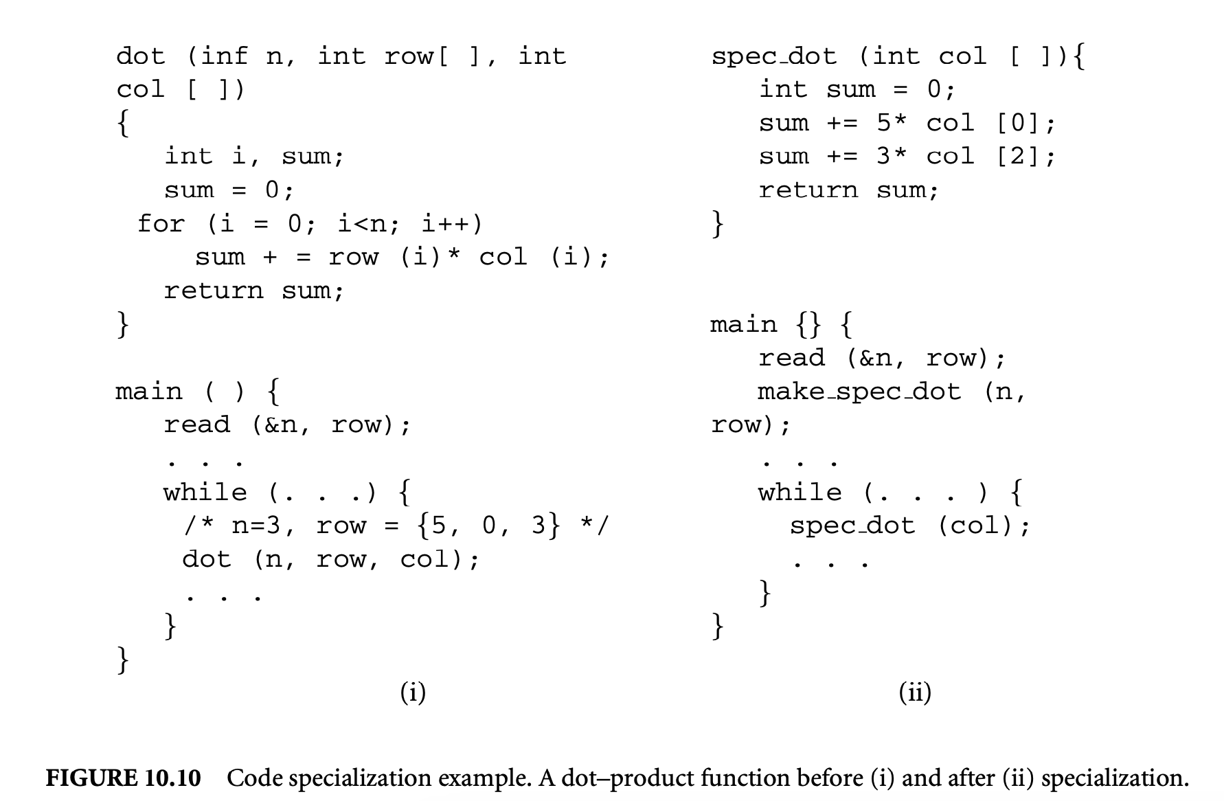
fills in the holes for parameters and row with their runtime values, and patches the original main routine to link in the new specialized code.
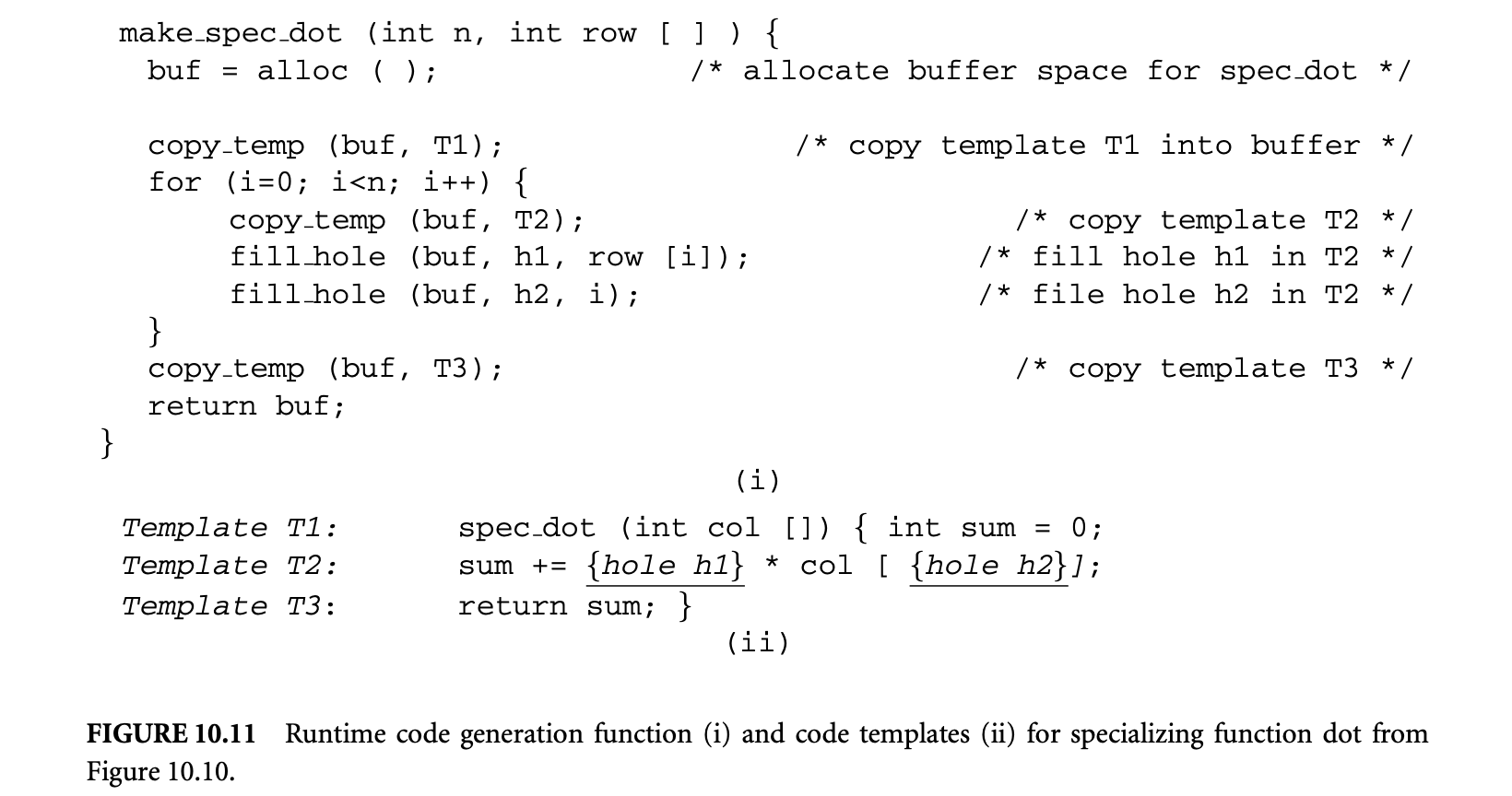 The required compiler support renders these runtime specialization techniques less flexible than transparent dynamic compilation systems. The kind, scope, and timing of dynamic code generation are fixed at compile time and hardwired into the code. Furthermore, runtime code specialization techniques usually require programmer assistance to choose the specialization regions and variables (e.g., via code annotations or compiler directives). Because overspecialization can easily result in code explosion and performance degradation, the selection of beneficial specialization candidates is likely to follow an interactive approach,
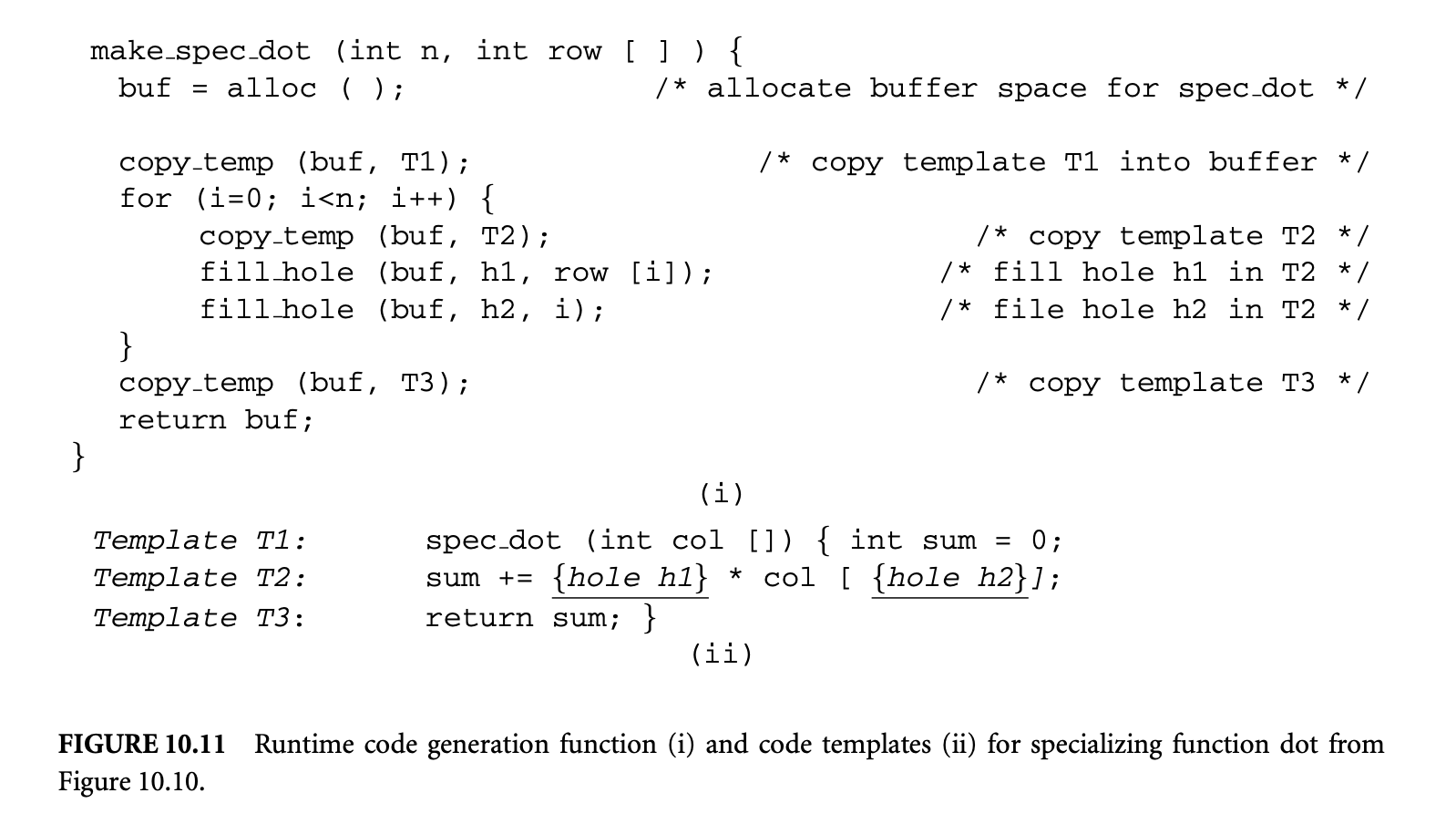 where the programmer explores various specialization opportunities. Recently, a system has been developed toward automating the placement of compiler directives for dynamic code specialization [32].
The preceding techniques for runtime specialization are classified as declarative. Based on the programmer declaration, templates are produced automatically by the static compiler. An alternative approach is imperative code specialization. In an imperative approach, the programmer explicitly encodes the runtime templates. C is an extension of the C languages that allows the programmer to specify dynamic code templates [33]. The static compiler compiles these programmer specifications into code templates that are initiated at runtime in a similar way to the declarative approach. Imperative runtime specialization is more general because it can support a broader range of runtime code generation techniques. However, it also requires deeper programmer involvement and is more error prone, because of the difficulty of specifying the dynamic code templates.
10.7 Summary
Dynamic compilation is a growing research field fueled by the desire to go beyond the traditional compilation model that views a compiled binary as a static immutable object. The ability to manipulate and transform code at runtime provides the necessary instruments to implement novel execution services. This chapter discussed the mechanisms of dynamic compilation systems in the context of two applications: dynamic performance optimization and transparent software migration. However, the capabilities of dynamic compilation systems can go further and enable such services as dynamic decompression and decryption or the implementation of security policies and safety checks.
Dynamic compilation should not be viewed as a technique that competes with static compilation. Dynamic compilation complements static compilation, and together they make it possible to move toward a truly write-once-run-anywhere paradigm of software implementation.
Although dynamic compilation research has advanced substantially in recent years, numerous challenges remain. Little progress has been made in providing effective development and debugging support for dynamic compilation systems. Developing and debugging a dynamic compilation system is particularly difficult because the source of program bugs may be inside transient dynamically generated code. Break points cannot be placed in code that has not yet materialized, and symbolic debugging of dynamically generated code is not an option. The lack of effective debugging support is one of the reasons the engineering of dynamic compilation systems is such a difficult task. Another area that needs further attention is code validation. Techniques are needed to assess the correctness of dynamically generated code. Unless dynamic compilation systems can guarantee high levels of robustness, they are not likely to achieve widespread adoption.
This chapter surveys and discusses the major approaches to dynamic compilation with a focus on transparent binary dynamic compilation. For more information on the dynamic compilation systems that have been discussed, we encourage the reader to explore the sources cited in the References section.
References
L. Anderson, M. Berc, J. Dean, M. Ghemawat, S. Henzinger, S. Leung, L. Sites, M. Vandervoorde, C. Waldspurger, and W. Weihl. 1977. Continuous profiling: Where have all the cycles gone? In Proceedings of the 16th ACM Symposium of Operating Systems Principles, 14. 2: D. Bruening and E. Duesterwald. 2000. Exploring optimal compilation unit shapes for an embedded just-in-time compiler. In Proceedings of the 3rd Workshop on Feedback-Directed and Dynamic Optimization. 3: D. Bruening, E. Duesterwald, and S. Amarasinghe. 2001. Design and implementation of a dynamic optimization framework for Windows. In Proceedings of the 4th Workshop on Feedback-Directed and Dynamic Optimization. 4: V. Bala, E. Duesterwald, and S. Banerjia. 1999. Transparent dynamic optimization: The design and implementation of Dynamo. Hewlett-Packard Laboratories Technical Report HPL-1999-78.
V. Bala, E. Duesterwald, and S. Banerjia. 2000. Dynamo: A transparent runtime optimization system. In Proceedings of the SIGPLAN '00 Conference on Programming Language Design and Implementation, 1-12. 6: T. Ball and J. Larus. 1996. Efficient path profiling. In Proceedings of the 29th Annual International Symposium on Microarchitecture (MICRO-29), 46-57. 7: W. Chen, S. Lerner, R. Chaiken, and D. Gillies. 2000. Mojo: A dynamic optimization system. In Proceedings of the 3rd Workshop on Feedback-Directed and Dynamic Optimization. 8: R. F. Cmelik and D. Keppel. 1993. Shade: A fast instruction set simulator for execution profiling. Technical Report UWCSE-93-06-06, Department of Computer Science and Engineering, University of Washington, Seattle. 9: C. Consel and F. Noel. 1996. A general approach for run-time specialization and its application to C. In Proceedings of the 23rd Annual Symposium on Principles of Programming Languages, 145-56. 10: T. Conte, B. Patel, K. Menezes, and J. Cox. 1996. Hardware-based profiling: an effective technique for profile-driven optimization. Int. J. Parallel Programming 24:187-206. 11: C. Chambers and D. Ungar. 1989. Customization: Optimizing compiler technology for SELF, a dynamically-typed object-oriented programming language. In Proceedings of the SIGPLAN '89 Conference on Programming Language Design and Implementation, 146-60. 12: Y. C. Chung and Y. Byung-Sun. The Latte Java Virtual Machine. Mass Laboratory, Seoul National University, Korea. latte.snu.ac.kr/manual/html mono/latte.html. 13: R. Cohn and G. Lowney. 1996. Hot cold optimization of large Windows/NT applications. In Proceedings of the 29th Annual International Symposium on Microarchitecture, 80-89. 14: D. Ditzel. 2000. Transmeta's Crusoe: Cool chips for mobile computing. In Proceedings of Hot Chips 12, Stanford University, Stanford, CA. 15: D. Deaver, R. Gorton, and N. Rubin. 1999. Wiggins/Redstone: An online program specializer. In Proceedings of Hot Chips 11, Palo Alto, CA. 16: E. Duesterwald and V. Bala. 2000. Software profiling for hot path prediction: Less is more. In Proceedings of 9th International Conference on Architectural Support for Programming Languages and Operating Systems, 202-211. 17: E. Duesterwald, R. Gupta, and M. L. Soffa. 1995. Demand-driven computation of interprocedural data flow. In Proceedings of the 22nd ACM Symposium on Principles on Programming Languages. 37-48. 18: L. P. Deutsch and A. M. Schiffman. 1994. Efficient implementation of the Smalltalk-80 system. In Conference Record of the 11th Annual ACM Symposium on Principles of Programming Languages, 297-302. 19: K. Ebcioglu and E. Altman. 1997. DAISY: Dynamic compilation for 100% architectural compatibility. In Proceedings of the 24th Annual International Symposium on Computer Architecture, 26-37. 20: D. R. Engler. 1996. VOODE: A retargetable, extensible, very fast dynamic code generation system. In Proceedings of the SIGPLAN '96 Conference on Programming Language Design and Implementation (PLDI '96), 160-70. 21: D. H. Friendly, S. J. Patel, and Y. N. Patt. 1998. Putting the fill unit to work: Dynamic optimizations for trace cache microprocessors. In Proceedings of the 31st Annual International Symposium on Microarchitecture (MICRO-31), 173-81. 22: J. Gosling, B. Joy, and G. Steele. 1999. The Java language specification. Reading, MA: Addison-Wesley. 23: B. Grant, M. Philipose, M. Mock, C. Chambers, and S. Eggers. 1999. An evaluation of staged run-time optimizations in DyC. In Proceedings of the SIGPLAN '99 Conference on Programming Language Design and Implementation, 293-303. 24: M. Gschwind and E. Altman. 2000. Optimization and precise exceptions in dynamic compilation. In Proceedings of Workshop on Binary Translation.
U. Hoelzle, C. Chambers, and D. Ungar. 1991. Optimizing dynamically-typed object-oriented languages with polymorphic inline caches. In Proceedings of ECOOP 4th European Conference on Object-Oriented Programming, 21-38. 26: U. Hoelzle, C. Chambers, and D. Ungar. 1992. Debugging optimized code with dynamic deoptimization. In Proceedings of the SIGPLAN '92 Conference on Programming Language Design and Implementation, 32-43. 27: R. J. Hookway and M. A. Herdeg. 1997. FXl32: Combining emulation and binary translation. Digital Tech. J. 0(1):3-12. 28: IBM Research. The IBM Jalapeno Project. <www.research.ibm.com/jalapeno/>. 29: Intel Microprocessor Research Lab. Open Runtime Platform. <www.intel.com/research/mrl/orp/>. 30: C. Krintz and B. Calder. 2001. Usingannotations to reduce dynamic optimization time. In Proceedings of the SIGPLAN '01 Conference on Programming Language Design and Implementation, 156-67. 31: M. Leone and P. Lee. 1996. Optimizing ML with run-time code generation. In Proceedings of the SIGPLAN '96 Conference on Programming Language Design and Implementation, 137-48. 32: M. Mock, M. Berryman, C. Chambers, and S. Eggers. 1999. Calpa: A tool for automatic dynamic compilation. In Proceedings of the 2nd Workshop on Feedback-Directed and Dynamic Optimization. 33: M. Poletta, D. R. Engler, and M. F. Kaashoek. 1997. TCC: A system for fast flexible, and high-level dynamic code generation. In Proceedings of the SIGPLAN '97 Conference on Programming Language Design and Implementation, 109-21. 34: S. Richardson. 1993. Exploiting trivial and redundant computation. In Proceedings of the 11th Symposium on Computer Arithmetic. 35: K. Scott and J. Davidson. 2001. Strata: A software dynamic translation infrastructure. In Proceedings of the 2001 Workshop on Binary Translation. 36: A. Srivastava, A. Edwards, and H. Vo. 2001. Vulcan: Binary translation in a distributed environment. Technical Report MSR-TR-2001-50, Microsoft Research. 37: O. Taub, S. Schechter, and M. D. Smith. 2000. Ephemeral instrumentation for lightweight program profiling. Technical report, Harvard University. 38: Transitive Technologies. <www.transitives.com/>. 39: D. Ung and C. Cifuentes. 2000. Machine-adaptable dynamic binary translation. ACM Sigplan Notices 35(7):41-51. 40: X. Zhang, Z. Wang, N. Gloy, J. Chen, and M. Smith. 1997. System support for automatic profiling and optimization. In Proceedings of the 16th ACM Symposium on Operating Systems Principles, 15-26.
Chapter 15 Computations on Iteration Spaces
15.1 Introduction
This chapter consists of two independent parts. The first deals with programs involving indexed data sets such as dense arrays and indexed computations such as loops. Our position is that high-level mathematical equations are the most natural way to express a large class of such computations, and furthermore, such equations are amenable to powerful static analyses that would enable a compiler to derive very efficient code, possibly significantly better than what a human would write. We illustrate this by describing a simple equational language and its semantic foundations and by illustrating the analyses we can perform, including one that allows the compiler to reduce the degree of the polynomial complexity of the algorithm embodied in the program.
The second part of this chapter deals with tiling, an important program reordering transformation applicable to imperative loop programs. It can be used for many different purposes. On sequential machines tiling can improve the locality of programs by exploiting reuse, so that the caches are used more effectively. On parallel machines it can also be used to improve the granularity of programs so that the communication and computation "units" are balanced.
We describe the tiling transformation, an optimization problem for selecting tile sizes, and how to generate tiled code for codes with regular or affine dependences between loop iterations. We also discuss approaches for reordering iterations, parallelizing loops, and tiling sparse computations that have irregular dependences.
15.2 The -Polyhedral Model and Some Static Analyses
It has been widely accepted that the single most important attribute of a programming language is programmer productivity. Moreover, the shift to multi-core consumer systems, with the number of cores expected to double every year, necessitates the shift to parallel programs. This emphasizes the need for productivity even further, since parallel programming is substantially harder than writing unithreadedcode. Even the field of high-end computing, typically focused exclusively on performance, is becoming concerned with the unacceptably high cost per megaflop of current high-end systems resulting from the required programming expertise. The current initiative is to increase programmability, portability, and robustness. DARPA's High Productivity Computing Systems (HPCSs) program aims to reevaluate and redesign the computing paradigms for high-performance applications from architectural models to programming abstractions.
We focus on compute- and data-intensive computations. Many data-parallel models and languages have been developed for the analysis and transformation of such computations. These models essentially abstract programs through (a) variables representing collections of values, (b) pointwise operations on the elements in the collections, and (c) collection-level operations. The parallelism may either be specified explicitly or derived automatically by the compiler. Parallelism detection involves analyzing the dependence between computations. Computations that are independent may be executed in parallel.
We present high-level mathematical equations to describe data-parallel computations succinctly and precisely. Equations describe the kernels of many applications. Moreover, most scientific and mathematical computations, for example, matrix multiplication, LU-decomposition, Cholesky factorization, Kalman filtering, as well as many algorithms arising in RNA secondary structure prediction, dynamic programming, and so on, are naturally expressed as equations.
It is also widely known that high-level programming languages increase programmer productivity and software life cycles. The cost of this convenience comes in the form of a performance penalty compared to lower-level implementations. With the subsequent improvement of compilation technology to accommodate these higher-level constructs, this performance gap narrows. For example, most programmers never use assembly language today. As a compilation challenge, the advantages of programmability offered by equations need to be supplemented by performance. After our presentation of an equational language, we will present automatic analyses and transformations to reduce the asymptotic complexity and to parallelize our specifications. Finally, we will present a brief description of the generation of imperative code from optimized equational specifications. The efficiency of the generated imperative code is comparable to hand-optimized implementations.
For an example of an equational specification and its automatic simplification, consider the following:
 Here, the variable is defined over a line segment, and the variables and , over a triangle and a square, respectively. These are the previously mentioned collections of values and are also called the domains of the respective variables. The dependence in the given computation is such that the value of at requires the value of at and the value of at for all valid values of and .
An imperative code segment that implements this equation is given in Figure 15.1. The triply nested loop (with linear bounds) indicates a asymptotic complexity for such an implementation. However, a implementation of Equation 15.1 exists and can be derived automatically. The code for this "simplified" specification is provided as well in Figure 15.1. The required sequence of transformations required to optimize the initial specification is given in Section 15.2.4. These transformations have been developed at the level of equations.
The equations presented so far have been of a very special form. It is primarily this special form that enables the development of sophisticated analyses and transformations. Analyses on general equations are often impossible. The class of equations that we consider consist of (a) variables defined on -polyhedral domains with (b) dependences in the form of affine functions. These restrictions enable us to use linear algebraic theory and techniques. In Section 15.2.1, we present -polyhedra and associated mathematical objects in detail that abstract the iteration domains of loop nests. Then we show the advantages of manipulating -polyhedra over integer polyhedra. A language to express equations over -polyhedral domains is presented in Section 15.2.3. The latter half of this section presents transformations to automatically simplify and parallelize equations. Finally, we provide a brief explanation of the transformations in the backend and code generation.
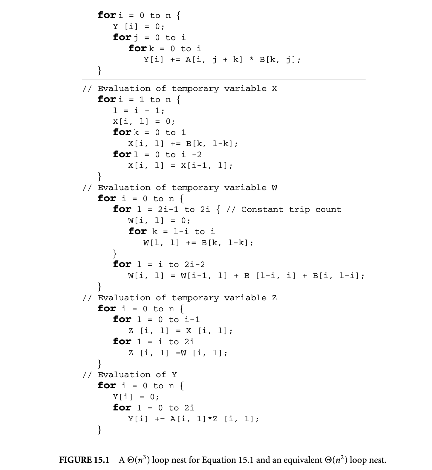
15.2.1 Mathematical Background1
Footnote 1: Parts of this section are adapted from [37], © 2007, Association for Computing Machinery, Inc., included by permission.
First, we review some mathematical background on matrices and decribe terminology. As a convention, we denote matrices with upper-case letters and vectors with lower-case. All our matrices and vectors have integer elements. We denote the identity matrix by . Syntactically, the different elements of a vector will be written as a list.
We use the following concepts and properties of matrices:
- The kernel of a matrix , written as , is the set of all vectors such that .
- The column (respectively row) rank of a matrix is the maximal number of linearly independent columns (respectively rows) of .
- A matrix is unimodular if it is square and its determinant is either or .
Figure 15: A loop nest for Equation 15.1 and an equivalent loop nest.
- Two matrices and are said to be column equivalent or right equivalent if there exists a unimodular matrix such that .
- A unique representative element in each set of matrices that are column equivalent is the one in Hermite normal form (HNF).
Definition 15.1:
An matrix with column rank is in HNF if:
-
For columns ,, , the first nonzero element is positive and is below the first positive element for the previous column.

-
In the first columns, all elements above the first positive element are zero.

-
The first positive entry in columns ,, is the maximal entry on its row. All elements are nonnegative in this row.

-
Columns are zero columns.

A template of a matrix in HNF is provided above. In the template, denotes the maximum element in the corresponding row, denotes elements that are not the maximum element, and denotes any integer. Both and are nonnegative elements.
For every matrix , there exists a unique matrix that is in HNF and column equivalent to , that is, there exists a unimodular matrix such that . Note that the provided definition of the HNF does not require the matrix to have full row rank.
15.2.1 Integer Polyhedra
An integer polyhedron, , is a subset of that can be defined by a finite number of affine inequalities (also called affine constraints or just constraints when there is no ambiguity) with integer coefficients. We follow the convention that the affine constraint is given as , where . The integer polyhedron, , satisfying the set of constraints , is often written as , where is an matrix and is a -vector.
Example 15.1:
Consider the equation
 The domains of the variables , , and are, respectively, the sets , , and . These sets are polyhedra, and deriving the aforementioned representation simply requires us to obtain, through elementary algebra, all affine constraints of the correct form, yielding , , and , respectively. Nevertheless, these are less intuitive, and in our presentation, we will not conform to the formalities of representation.
A subtle point to note here is that elements of polyhedral sets are tuples of integers. The index variables , , , and are simply place holders and can be substituted by other unused names. The domain of can also be specified by the set .
We shall use the following properties and notation of integer polyhedra and affine constraints:
- For any two coefficients and , where , and , is said to be a convex combination of and . If and are two iteration points in an integer polyhedron, , then any convex combination of and that has all integer elements is also in .
- The constraint of is said to be saturated iff.
- The lineality space of is defined as the linear part of the largest affine subspace contained in . It is given by .
- The context of is defined as the linear part of the smallest affine subspace that contains . If the saturated constraints in are the rows of , then the context of is .
15.2.1.1 Parameterized Integer Polyhedra
Recall Equation 15.1. The domain of is given by the set . Intuitively, the variable is seen as a size parameter that indicates the problem instance under consideration. If we associate every iteration point in the domain of with the appropriate problem instance, the domain of would be described by the set . Thus, a parameterized integer polyhedron is an integer polyhedron where some indices are interpreted as size parameters.
An equivalence relation is defined on the set of iteration points in a parameterized polyhedron such that two iteration points are equivalent if they have identical values of size parameters. By this relation, a parameterized polyhedron is partitioned into a set of equivalence classes, each of which is identified by the vector of size parameters. Equivalence classes correspond to program instances and are, thus, called instances of the parameterized polyhedron. We identify size parameters by omitting them from the index list in the set notation of a domain.
15.2.1.2 Affine Images of Integer Polyhedra
An (standard) affine function, , is a function from iteration points to iteration points. It is of the form , where is an matrix and is an -vector.
Consider the integer polyhedron and the standard affine function given above. The image of under is of the form . These are the so-called linearly bound lattices (LBLs). The family of LBLs is a strict superset of the family of integer polyhedra. Clearly, every integer polyhedra is an LBL with and . However, for an example of an LBL that is not an integer polyhedron refer to Figure 15.2.

Figure 15.2: The LBL corresponding to the image of the polyhedron by the affine function does not contain the iteration point 8 but contains 7 and 9. Since 8 is a convex combination of 7 and 9, the set is not an integer polyhedron. Adapted from [37], © 2007, Association for Computing Machinery, Inc., included by permission.
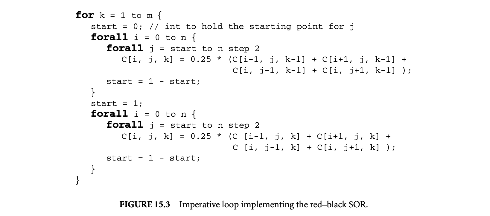
15.2.1.3 Affine Lattices
Often, the domain over which an equation is specified, or the iteration space of a loop program, does not contain every integer point that satisfies a set of affine constraints.
Example 15.2: Consider the red-black SOR for the iterative computation of partial differential equations. Iterations in the plane are divided into "red" points and "black" points, similar to the layout of squares in a chess board. First, black points (at even ) are computed using the four neighboring red points (at odd ), and then the red points are computed using its four neighboring black points. These two phases are repeated until convergence. Introducing an additional dimension, to denote the iterative application of the two phases, we get the following equation:
 where the domain of is , and are size parameters, and is given as input. The imperative loop nest that implements this equation is given in Figure 15.3.
We see that the first (respectively second) branch of the equation is not defined over all iteration points that satisfy a set of affine constraints, namely, , but over points that additionally satisfy (respectively ). This additional constraint in the first branch of the equation is satisfied precisely by the iteration points that can be expressed as an integer linear combination of the vectors . The vectors and are the generators of the lattice on which these iteration points lie.
The additional constraint in the second branch of the equation is satisfied precisely by iteration points that can be expressed as the following affine combination:
 Formally, the lattice generated by a matrix is the set of all integer linear combinations of the columns of . If the columns of a matrix are linearly independent, they constitute a basis of the generated lattice. The lattices generated by two-dimensionally identical matrices are equal iff the matrices are column equivalent. In general, the lattices generated by two arbitrary matrices are equal iff the submatrices corresponding to the nonzero columns in their HNF are equal.
As seen in the previous example, we need a generalization of the lattices generated by a matrix, additionally allowing offsets by constant vectors. These are called affine lattices. An affine lattice is a subset of of the form , where and are an matrix and -vector, respectively. We call the coordinates of the affine lattice.
The affine lattices and are equal iff the lattices generated by and are equal and for some constant vector . The latter requirement basically enforces that the offset of one lattice lies on the other lattice.
15.2.1.4 -Polyhedra
-polyhedron is the intersection of an integer polyhedron and an affine lattice. Recall the set of iteration points defined by either branch of the equation for the red-black SOR. As we saw above, these iteration points lie on an affine lattice in addition to satisfying a set of affine constraints. Thus, the set of these iteration points is precisely a -polyhedron. When the affine lattice is the canonical lattice, , a -polyhedron is also an integer polyhedron. We adopt the following representation for -polyhedra:
 where has full column rank, and the polyhedron has a context that is the universe, . is called the coordinate polyhedron of the -polyhedron. The -polyhedron for which has no columns has a coordinate polyhedron in .
We see that every -polyhedron is an LBL simply by observing that the representation for a -polyhedron is in the form of an affine image of an integer polyhedron. However, the LBL in Figure 15.2 is clearly not a -polyhedron. There does not exist any lattice with which we can intersect the integer polyhedron to get the set of iteration points of the LBL. Thus, the family of LBLs is a strict superset of the family of -polyhedra.
Our representation for -polyhedra as affine images of integer polyhedra is specialized through the restriction to and . We may interpret the -polyhedral representation in Equation 15.3 as follows. It is said to be based on the affine lattice given by . Iteration points of the -polyhedral domain are points of the affine lattice corresponding to valid coordinates. The set of valid coordinates is given by the coordinate polyhedron.
15.2.1.4.1 Parameterized -Polyhedra
parameterized -polyhedron is a -polyhedron where some rows of its corresponding affine lattice are interpreted as size parameters. An equivalence relation is defined on the set of iteration points in a parameterized -polyhedron such that two iteration points are equivalent if they have identical value of size parameters. By this relation, a parameterized -polyhedron is partitioned into a set of equivalence classes, each of which is identified by the vector of size parameters. Equivalence classes correspond to program instances and are, thus, called instances of the parameterized -polyhedron.
For the sake of explanation, and without loss of generality, we may impose that the rows that denote size parameters are before all non-parameter rows. The equivalent -polyhedron based on the HNF of such a lattice has the important property that all points of the coordinate polyhedron with identical values of the first few indices belong to the same instance of the parameterized -polyhedron.
Example 15.3
Consider the -polyhedron given by the intersection of the polyhedron and the lattice .1 It may be written as

For both the polyhedron and the affine lattice, the specification of the coordinate space is redundant. It can be derived from the number of indices and is therefore dropped for the sake of brevity.
Now, suppose the first index, , in the polyhedron is the size parameter. As a result, the first row in the lattice corresponding to the -polyhedron is the size parameter. The HNF of this lattice is . The equivalent -polyhedron is

The iterations of this -polyhedron belong to the same program instance iff they have the same coordinate index . Note that valid values of the parameter row trivially have a one-to-one correspondence with values of , identity being the required bijection. In the general case, however, this is not the case. Nevertheless, the required property remains invariant. For example, consider the following -polyhedron with the first two rows considered as size parameters:
 Here, valid values of the parameter rows have a one-to-one correspondence with the values of and , but it is impossible to obtain identity as the required bijection.
15.2.1.5 Affine Lattice Functions
Affine lattice functions are of the form , where has full column rank. Such functions provide a mapping from the iteration to the iteration . We have imposed that have full column rank to guarantee that be a function and not a relation, mapping any point in its domain to a unique point in its range. All standard affine functions are also affine lattice functions.
The mathematical objects introduced here are used to abstract the iteration domains and dependences between computations. In the next two sections, we will show the advantages of manipulating equations with -polyhedral domains instead of polyhedral domains and present a language for the specification of such equations.
15.2.2 The -Polyhedral Model
We will now develop the -polyhedral model that enables the specification, analysis, and transformation of equations described over -polyhedral domains. It has its origins in the polyhedral model that has been developed for over a quarter century. The polyhedral model has been used in a variety of contexts, namely, automatic parallelization of loop programs, locality, hardware generation, verification, and, more recently, automatic reduction of asymptotic computational complexity. However, the prime limitation of the polyhedral model lay in its requirement for dense iteration domains. This motivated the extension to -polyhedral domains. As we have seen in the red-black SOR, -polyhedral domains describe the iterations of a regular loop with non-unit stride.
In addition to allowing more general specifications, the -polyhedral model enables more sophisticated analyses and transformations by providing greater information in the specifications, namely, pertaining to lattices. The example below demonstrates the advantages of manipulating -polyhedral domains. The variable is defined over the domain .2
Code fragments in this section are adapted from [37], © 2007, Association for Computing Machinery, Inc., included by permission.
 In the loop, only iteration points that are a multiple of 2 or 3 execute the statement . The iteration at may be excluded from the loop nest. Generalizing, any iteration that can be written in the form may be excluded from the loop nest. The same argument applies to iterations that can be written in the form . As result of these "holes," all iterations at may be executed in parallel at the first time step. The iterations at may also be executed in parallel at the first time step. At the next time step, we may execute iterations at and finally at iterations . The length of the longest dependence chain is 3. Thus, the loop nest can be parallelized to execute in constant time as follows:
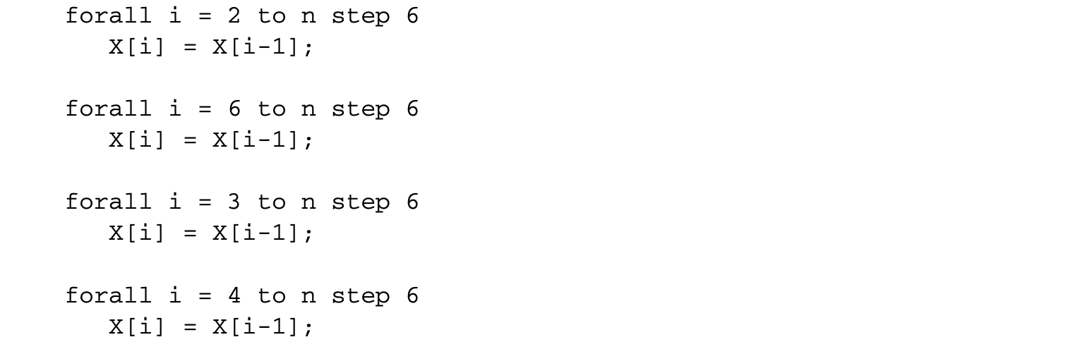 However, our derivation of parallel code requires to manipulate -polyhedral domains. A polyhedral approximation of the problem would be unable to result in such a parallelization.
Finally, the -polyhedral model allows specifications with a more general dependence pattern than the specifications in the polyhedral model. Consider the following equation that cannot be expressed in the polyhedral model.
 where and the corresponding loop is
 This program exhibits a dependence pattern that is richer than the affine dependences of the polyhedral model. In other words, it is impossible to write an equivalent program in the polyhedral model, that is, without the use of the mod operator or non-unit stride loops, that can perform the required computation. One may consider replacing the variable with two variables and corresponding to the even and odd points of such that and . However, the definition of now requires the mod operator, because and .
Thus, the -polyhedral model is a strict generalization of the polyhedral model and enables more powerful optimizations.
15.2.3 Equational Language
In our presentation of the red-black SOR in Section 15.2.1.3, we studied the domains of the two branches of Equation 15.2. More specifically, these are the branches of the case expression in the right-hand side (rhs) of the equation. In general, our techniques require the analysis and transformation of the subexpressions that constitute the rhs of equations, treating expressions as first-class objects.
For example, consider the simplification of Equation 15.1. As written, the simplification transforms the accumulation expression in the rhs of the equation. However, one would expect the technique to be able to decrease the asymptotic complexity of the following equation as well.
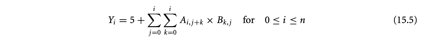 Generalizing, one would reasonably expect the existence of a technique to reduce the complexity of evaluation of the accumulation subexpression (), irrespective of its "level." This motivates a homogeneous treatment of the subexpression at any level. At the lowest level of specification,a subexpression is a variable (or a constant) associated with a domain. Generalizing, we associate domains to arbitrary subexpressions.
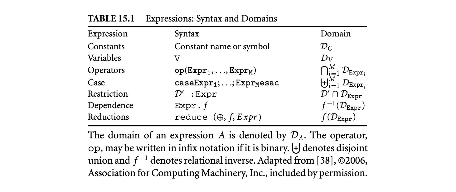 The treatment of expressions as first-class objects leads to the design of a functional language where programs are a finite list of (mutually recursive) equations of the form , where both Var and Expr denote mappings from their respective domains to a set of values (similar to multidimensional arrays). A variable is defined by at most one equation. Expressions are constructed by the rules given in Table 15.1, column 2. The domains of all variables are declared, the domains of constants are either declared or defined over by default, and the domains of expressions are derived by the rules given in Table 15.1, column 3. The function specified in a dependence expression is called the dependence function (or simply a dependence), and the function specified in a reduction is called the projection function (or simply a projection).
In this language, Equation 15.5 would be a syntactically sugared version of the following concrete problem.
 In the equation above, 5 is a constant expression defined over and Y, A, and B are variables. In addition to the equation, the domains of Y, A, and B would be declared as the sets , , and , respectively. The reduction expression is the accumulation in Equation 15.5. Summation is expressed by the reduction operator + (other possible reduction operators are *, max, min, or, and, etc.). The projection function (i,j,k->i) specifies that the accumulation is over the space spanned by and resulting in values in the one-dimensional space spanned by . A subtle and important detail is that the expression that is accumulated is defined over a domain in three-dimensional space spanned by , , and (this information is implicit in standard mathematical specifications as in Equation 15.5). This is an operator expression equal to the product of the value of at and at . In the space spanned by , , and , the required dependences on and are expressed through dependence expressions A.(i,j,k->i,j+k) and B.(i,j,k->k,j), respectively. The equation does not contain any case or restrict constructs. For an example of these two constructs, refer back to Equation 15.4. In our equational specification, the equation would be written as
 where the domains of and the constant are and , respectively. There are two branches of the case expression, each of which is a restriction expression. We have not provided domains of any of the subexpressions mentioned above for the sake of brevity. These can be computed using the rules given in Table 15.1, column 3.
15.2.3.1
Parts of this section are adapted from [38], © 2006, Association for Computing Machinery, Inc., included by permission.
At this point3, we intuitively understand the semantics of expressions. Here, we provide the formal semantics of expressions over their domains of definition. At the iteration point in its domain, the value of:
- A constant expression is the associated constant.
- A variable is either provided as input or given by an equation; in the latter case, it is the value, at , of the expression on its rhs.
- An operator expression is the result of applying on the values, at , of its expression arguments. is an arbitrary, iteration-wise, single valued function.
- A case expression is the value at of that alternative, to whose domain belongs. Alternatives of a case expression are defined over disjoint domains to ensure that the case expression is not under- or overdefined.
- A restriction over is the value of at .
- The dependence expression is the value of at . For the affine lattice function , the value of the (sub)expression at equals the value of at .
- is the application of on the values of at all iteration points in that map to by . Since is an associative and commutative binary operator, we may choose any order of its application.
It is often convenient to have a variable defined either entirely as input or only by an equation. The former is called an input variable and the latter is a computed variable. So far, all our variables have been of these two kinds only. Computed variables are just names for valid expressions.
15.2.3.2 The Family of Domains
Variables (and expressions) are defined over -polyhedral domains. Let us study the compositional constructs in Table 15.1 to get a more precise understanding of the family of -polyhedral domains.
For compound expressions to be defined over the same family of domains as their subexpressions, the family should be closed under intersection (operator expressions, restrictions), union (case expression), and preimage (dependence expressions) and image (reduction expressions) by the family of functions. With closure, we mean that a (valid) domain operation on two elements of the family of domains should result in an element that also belongs to the family. For example, the family of integer polyhedra is closed under intersection but not under images, as demonstrated by the LBL in Figure 15.2. The family of integer polyhedra is closed under intersection since the intersection of two integer polyhedra that lie in the same dimensional space results in an integer polyhedron that satisfies the constraints of both the integer polyhedra.
In addition to intersection, union, and preimage and image by the family of functions, most analyses and transformations (e.g., simplification, code generation, etc.) require closure under the difference of two domains. With closure under the difference of domains, we may always transform any specification to have only input and computed variables.
The family of -polyhedral domains should be closed under the domain operations mentioned above. This constraint is unsatisfied if the elements of this family are -polyhedra. For example, the union of two -polyhedra is not a -polyhedron. Also, the LBL in Figure 15.2 shows that the image of a -polyhedron is not a -polyhedron. However, if the elements of the family of -polyhedral domains are unions of -polyhedra, then all the domain operations mentioned above maintain closure.
15.2.3.3 Parameterized Specifications
Extending the concept of parameterized -polyhedra, it is possible to parameterize the domains of variables and expressions with size parameters. This leads to parameterized equational specifications. Instances of the parameterized -polyhedra correspond to program instances.
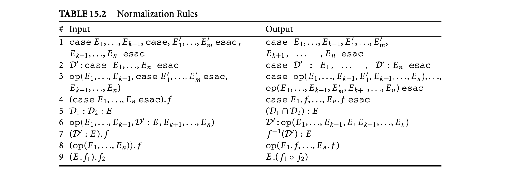 Every program instance in a parameterized specification is independent, so all functions should map consumer iterations to producer iterations within the same program instance.
15.2.3.4 Normalization
For most analyses and transformations (e.g., the simplification of reductions, scheduling, etc.), we need equations in a special normal form. Normalization is a transformation of an equational specification to obtain an equivalent specification containing only equations of the canonic forms or , where the expression is of the form
 and is a variable or a constant.
Such a normalization transformation4 first introduces an equation for every reduce expression, replacing its occurrence with the corresponding local variable. As a result, we get equations of the forms or , where the expression does not contain any reduce subexpressions. Subsequently, these expressions are processed by a rewrite engine to obtain equivalent expressions of the form specified in Equation 15.6. The rules for the rewrite engine are given in Table 15.2. Rules 1 to 4 "bubble" a single case expression to the outermost level, rules 5 to 7 then "bubble" a single restrict subexpression to the second level, rule 8 gets the operator to the penultimate level, and rule 9 is a dependence composition to obtain a single dependence at the innermost level.
and is a variable or a constant.
Such a normalization transformation4 first introduces an equation for every reduce expression, replacing its occurrence with the corresponding local variable. As a result, we get equations of the forms or , where the expression does not contain any reduce subexpressions. Subsequently, these expressions are processed by a rewrite engine to obtain equivalent expressions of the form specified in Equation 15.6. The rules for the rewrite engine are given in Table 15.2. Rules 1 to 4 "bubble" a single case expression to the outermost level, rules 5 to 7 then "bubble" a single restrict subexpression to the second level, rule 8 gets the operator to the penultimate level, and rule 9 is a dependence composition to obtain a single dependence at the innermost level.
More sophisticated normalization rules may be applied, expressing the interaction of reduce expressions with other subexpressions. However, these are unnecessary in the scope of this chapter.
The validity of these rules, in the context of obtaining a valid specification of the language, relies on the closure properties of the family of unions of -polyhedra.
15.2.4 Simplification of Reductions
Parts of this section are adapted from [38], © 2006, Association for Computing Machinery, Inc., included by permission.
We now provide a deeper study of reductions5. Reductions, commonly called accumulations, are the application of an associative and commutative operator to a collection of values to produce a collection of results.
Our use of equations was motivated by the simplification of asymptotic complexity of an equation involving reductions. We first present the required steps for the simplification. Then we will provide an intuitive explanation of the algorithm for simplification. For the sake of intuition, we use the standard mathematical notation for accumulations rather than the reduce expression.
Our initial specification was
 The loop nest corresponding to this equation has a complexity. The cubic complexity for this equation can also be directly deduced from the equational specification. Parameterized by , there are three independent7 indices within the summation. The following steps are involved in the derivation of the equivalent specification.
Footnote 7: With independent, we mean that there are no equalities between indices.
-
Introduce the index variable and replace every occurrence of with . This is a change of basis of the three-dimensional space containing the domain of the expression that is reduced.

The change in the order of summation is legal under our assumption that the reduction operator is associative and commutative.
-
Distribute multiplication over the summation since is independent of , the index of the inner summation.

-
Introduce variable to hold the result of the inner summation
 Note that the complexity of evaluating is now quadratic. However, we still have an equational specification that has cubic complexity (for the evaluation of ).
 -
Separate the summation over to remove min and max operators in the equation for .

-
Introduce variables and for each branch of the equation defining .
 Both the equations given above have cubic complexity.
 -
Reuse. The complexity for the evaluation of can be decreased by identifying that the expression on the rhs is independent of . We may evaluate each result once (for instance, at a boundary) and then pipeline along as follows.
 The initialization takes quadratic time since there are a linear number of results to evaluate and each evaluation takes linear time. Then the pipelining of results over an area requires quadratic time. This decreases the overall complexity of evaluating to quadratic time.
 -
Scan detection. The simplification of occurs when we identify
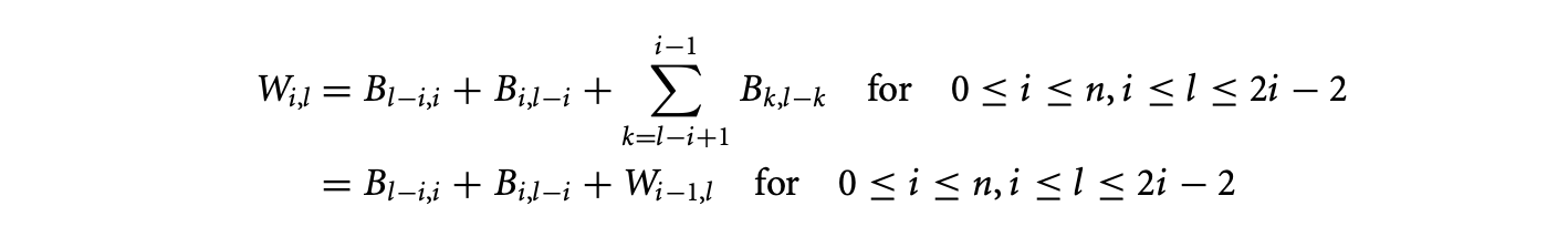 The values are, once again, initialized in quadratic time at a boundary (here, ). The scan takes constant time per iteration over an area and can be performed in quadratic time as well, thereby decreasing the complexity for the evaluation of to quadratic time.
 -
Summarizing, we have the following system of equations:
 These equations directly correspond to the optimized loop nest given in Figure 15. We have not optimized these equations or the loop nest any further for the sake for clarity, and moreso, because we only want to show an asymptotic decrease in complexity. However, a constant-fold improvement in the asymptotic complexity (as well as the memory requirement) can be obtained by eliminating the variable (or, alternatively, the two variables and ).
We now provide an intuitive explanation of the algorithm for simplification. Consider the reduction
 where is defined over the domain . The accumulation space of the above equation is characterized by . Any two points and that contribute to the same element of the result, , satisfy . To aid intuition, we may also write this reduction as
 is the "accumulation," using the operator, of the values of at all points that have the same image . Now, if has a distinct value at all points in its domain, they must all be computed, and no optimization is possible. However, consider the case where the expression exhibits reuse: its value is the same at many points in . Reuse is characterized by , the kernel of a many-to-one affine function, ;
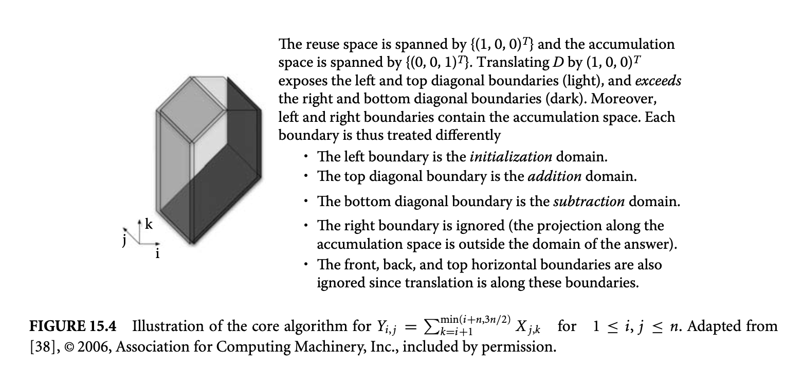 the value of at any two points in is the same if their difference belongs to . We can denote this reuse by , where is a variable with domain . In our language, this would be expressed by the dependence expression . The canonical equation that we analyze is
 Its nominal complexity is the cardinality of the domain of . The main idea behind our method is based on analyzing (a) , the domain of the expression inside the reduction, (b) its reuse space, and (c) the accumulation space.
15.2.4.1 Core Algorithm
Consider two adjacent instances of the answer variable, and along , where is a vector in the reuse space of . The set of values that contribute to and overlap. This would enable us to express in terms of . Of course, there would be residual accumulations on values outside the intersection that must be "added" or "subtracted" accordingly. We may repeat this for other values of along . The simplification results from replacing the original accumulation by a recurrence on and residual accumulations. For example, in the simple scan, , the expression inside the summation has reuse along . Taking , we get .
The geometric interpretation of the above reasoning is that we translate by a vector in the reuse space of . Let us call the translated domain . The intersection of and is precisely the domain of values, the accumulation over which can be avoided. Their differences account for the residual accumulations. In the simple scan explained above, the residual domain to be added is , and the domain to be subtracted is empty. The residual accumulations to be added or subtracted are determined only by and .
This leads to Algorithm 15.1 (also see Figure 15.4).
Algorithm 15.1 Intuition of the Core Algorithm6
Adapted from [38], © 2006, Association for Computing Machinery, Inc., included by permission.
- Choose , a vector in , along which the reuse of is to be exploited. In general, is multidimensional and therefore there may be infinitely many choices.
- Determine the domains , and corresponding to the domain of initialization, and the residual domains to subtract and to add, respectively. The choice of is made such that the cardinalities of these three domains are polynomials whose degree is strictly less than that for the original accumulation. This leads to simplification of the complexity.
Figure 15.4: Illustration of the core algorithm for for . Adapted from [38], © 2006, Association for Computing Machinery, Inc., included by permission.
- For these three domains, , , and , define the three expressions, , , and , consisting of the original expression , restricted to the appropriate subdomain.
- Replace the original equation by the following recurrence:

- Apply steps 1 to 4 recursively on the residual reductions over , , or if they exhibit further reuse.
Note that Algorithm 15.1 assumes that the reduction operation admits an inverse; that is, "subtraction" is defined. If this is not the case, we need to impose constraints on the direction of reuse to exploit: essentially, we require that the domain is empty. This leads to a feasible space of exploitable reuse.
15.2.4.2 Multidimensional Reuse
When the reuse space as well as the accumulation space are multidimensional, there are some interesting interactions. Consider the equation for . It has two-dimensional reuse (in the plane), and the accumulation is also two-dimensional (in the plane). Note that the two subspaces intersect, and this means that in the direction, not only do all points have identical values, but they also all contribute to the same answer. From the bounds on the summation we see that there are exactly such values, so the inner summation is just , because multiplication is a higher-order operator for repeated addition of identical values (similar situations arise with other operators, e.g., power for multiplication, identity for the idempotent operator max, etc.). We have thus optimized the computation to . However, our original equation had two dimensions of reuse, and we may wonder whether further optimization is possible. In the new equation , the body is the product of two subexpressions, and . They both have one dimension of reuse, in the and directions, respectively, but their product does not. No further optimization is possible for this equation.
However, if we had first exploited reuse along , we would have obtained the simplified equation , initialized with . The residual reduction here is itself a scan, and we may recurse the algorithm to obtain and initialized with . Thus, our equation can be computed in linear time. This shows how the choice of reuse vectors to exploit, and their order, affects the final simplification.
15.2.4.3 Decomposition of Accumulation
Consider the equation for . The one-dimensional reuse space is along , and is the two-dimensional accumulation space. The set of points that contribute to the th result lie in an rectangle of the two-dimensional input array . Comparing successive rectangles, we see that as the width decreases from one to the other, the height increases (Figure 15.5). If the operator does not have an inverse, it seems that we may not be able to simplify this equation. This is not true: we can see that for each we have an independent scan. The inner reduction is just a family of scans, which can be done in quadratic time with initialized with . The outer reduction just accumulates columns of , which is also quadratic.
What we did in this example was to decompose the original reduction that was along the space into two reductions, the inner along the space yielding partial answers along the plane and the outer that combined these partial answers along the space. Although the default choice of the decomposition -- the innermost accumulation direction -- of the space worked for this example, in general this is not the case. It is possible that the optimal solution may require a nonobvious decomposition, for instance,along some diagonal. We encourage the reader to simplify7 the following equation:
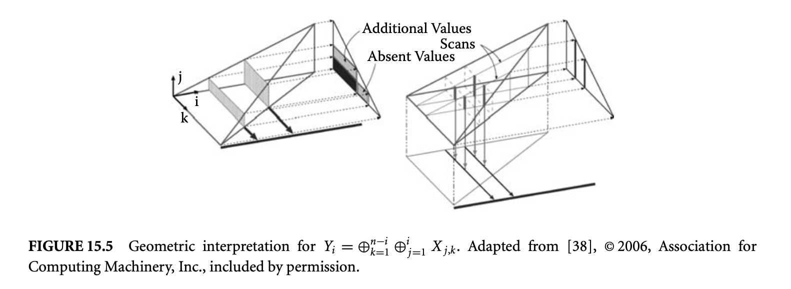
Solution: The inner reduction would map all points for which , for a given constant , to the same partial answer.

15.2.4.4 Distributivity and Accumulation Decomposition
Returning to the simplification of Equation 15.7, we see that the methods presented so far do not apply, since the body of the summation, , has no reuse. The expression has a distinct value at each point in the three-dimensional space spanned by , , and . However, the expression is composed of two subexpressions, which individually have reuse and are combined with the multiplication operator that distributes over the reduction operator, addition.
We may be able to distribute a subexpression outside a reduction if it has a constant value at all the points that map to the same answer. This was ensured by a change in basis of the three-dimensional space to , , and , followed by a decomposition to summations over and then . Values of were constant for different iterations of the accumulation over . After distribution, the body of the inner summation exhibited reuse that was exploited for the simplification of complexity.
15.2.5 Scheduling8
Adapted from [36] © 2007 IEEE, included by permission.
Scheduling is assigning an execution time to each computation so that precedence constraints are satisfied. It is one of the most important and widely studied problems. We present the scheduling analysis for programs in the -polyhedral model. The resultant schedule can be subsequently used to construct a space-time transformation leading to the generation of sequential or parallel code. The application of this schedule is made possible as a result of closure of the family of -polyhedral domains under image by the constructed transformation. We showed the advantages of scheduling programs in the -polyhedral model in Section 15.2.2. The general problem of scheduling programs with reductions is beyond the scope of this chapter. We will restrict our analysis to -polyhedral programs without reductions.
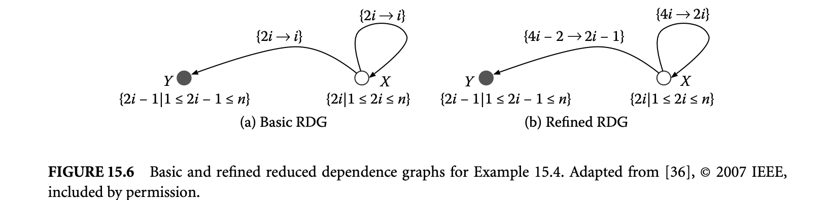
The steps involved in the scheduling analysis are (a) deriving precedence (causality) constraints for programs written in the -polyhedral model and (b) formulation of an integer linear program to obtain the schedule.
The precedence constraints between variables are derived from the reduced dependence graph (RDG). We will now provide some refinements of the RDG.
15.2.5.1 Basic and Refined RDG
Equations in the -polyhedral model can be defined over an infinite iteration domain. For any dependence analysis on an infinite graph, we need a compact representation. A directed multi-graph, the RDG precisely describes the dependences between iterations of variables. It is based on the normalized form of a specification and defined as follows:
- For every variable in the normalized specification, there is a vertex in the RDG labeled by the variable name and annotated by its domain. We will refer to vertices and variables interchangeably.
- For every dependence of the variable on , there is an edge from to , annotated by the corresponding dependence function. We will refer to edges and dependences interchangeably.
At a finer granularity, every branch of an equation in a normalized specification dictates the dependences between computations. A precise analysis requires that dependences be expressed separately for every branch. Again, for reasons of precision, we may express dependences of a variable separately for every -polyhedron in the -polyhedral domain of the corresponding branch of its equation. To enable these, we replace a variable by a set of new variables as elaborated below. Remember, our equations are of the form
 Let be written as a disjoint union of -polyhedra given by . The variable in the domain is replaced by a new variable, for instance, . Similarly, let be replaced by new variables given as . The dependence of in on is replaced by dependences from all on all . An edge from to may be omitted if there are no iterations in that map to (mathematically, if the preimage of by the dependence function does not intersect with ). A naive construction following these rules results in the basic reduced dependence graph.
Figure 15.6a gives the basic RDG for Equation 15.4, which is repeated here for convenience.
 The domains of and the constant are and , respectively. Next, we will study a refinement on this RDG.
In the RDG for the generic equation given in Equation 15.10, let be a variable derived from and defined on , and let be a variable derived from defined on , where and are given as follows:

A dependence of the form is directed from to . at cannot be evaluated before at . The affine lattice may contain points that do not lie in the affine lattice . Similarly, the affine lattice may contain points that do not lie in the affine lattice . As a result, the dependence may be specified on a finer lattice than necessary and may safely be replaced by a dependence of the form , where
 where and are matrices and and are integer vectors. The refined RDG is a refinement of the basic RDG where every dependence has been replaced by a dependence satisfying Equation 15.11. Figure 15.6b gives the refined RDG for Equation 15.4.
15.2.5.2 Causality Constraints
Dependences between the different iterations of variables impose an ordering on their evaluation. A valid schedule of the evaluation of these iterations is the assignment of an execution time to each computation so that precedence (causality) constraints are satisfied.
Let and be two variables in the refined RDG defined on and , respectively. We seek to find schedules on and of the following form:
 where and are affine functions on and , respectively. Our motivation for such schedules is that all vectors and matrices are composed of integer scalars. If we seek schedules of the form , where is an affine function and is an iteration in the domain of a variable, then we may potentially assign execution times to "holes," or computations that do not exist.
We will now formulate causality constraints using the refined RDG. Consider dependences from to . All such dependences can be written as
 where and are matrices and and are vectors. The execution time for at should precede the execution time for at . With the nature of the schedules presented in Equation 15.12, our causality constraint becomes
 with the assumption that op is atomic and takes a single time step to evaluate.
From these constraints, we may derive an integer linear program to obtain schedules of the form , where is the lattice corresponding to the -polyhedron and is the affine function (composed of integer scalars) on the coordinates of this lattice. An important feature of this formulation is that the resultant schedule can then be used to construct a space-time transformation.
15.2.6 Backend
After optimization of the equational specification and obtaining a schedule, the following steps are performed to generate (parallel) imperative code.
Analogous to the schedule that assigns a date to every operation, a second key aspect of the parallelization is to assign a processor to each operation. This is done by means of a processor allocation function. As with schedules, we confine ourselves to affine lattice functions. Since there are no causality constraints for choosing an allocation function, there is considerable freedom in choosing it. However, in the search for processor allocation functions, we need to ensure that two iteration points that are scheduled at the same time are not mapped to the same processing element.
The final key aspect in the static analysis of our equations is the allocation of operations to memory locations. As with the schedule and processor allocation function, the memory allocation is also an affine lattice function. The memory allocation function is, in general, a many-to-one mapping with most values overwritten as the computation proceeds. The validity condition for memory allocation functions is that no value is overwritten before all the computations that depend on it are themselves executed.
Once we have the three sets of functions, namely, schedule, processor allocation, and memory allocation, we are left with the problem of code generation. Given the above three functions, how do we produce parallel code that "implements" these choices? Code generation may produce either sequential or parallel code for programmable processors, or even descriptions of application-specific or nonprogrammable hardware (in appropriate hardware description language) that implements the computation specified by the equation.
Current techniques in code generation produce extremely efficient implementations comparable to hand-optimized imperative programs. With this knowledge, we return to our motivation for the use of equations to specify computations. An imperative loop nest that corresponds to an equation contains more information than required to specify the computation. There is an order (corresponding to the schedule) in the evaluation of values of a variable at different iteration points, namely, the lexicographic order of the loop indices. A loop nest also specifies the order of evaluation of the partial results of accumulations. A memory mapping has been chosen to associate values to memory locations. Finally, in the case of parallel code, a loop nest also specifies a processor allocation. Any analysis or transformation of loop nests that is equivalent to analysis or transformations on equations has to deconstruct these attributes and, thus, becomes unnecessarily complex.
15.2.7 Bibliographic Notes9
Parts of this section are adapted from [36] © 2007 IEEE and [37, 38], © 2007, 2006 Association for Computing Machinery, Inc., included by permission.
Our presentation of the equational language and the various analyses and transformations is based on the the ALPHA language [59, 69] and the MMALPHA framework for manipulating ALPHA programs, which relies on a library for manipulating polyhedra [107].
Although the presentation in this section has focused on equational specifications, the impact of the presented work is equally directed toward loop optimizations. In fact, many advances in the development of the polyhedral model were motivated by the loop parallelization and hardware synthesis communities.
To overcome the limitations of the polyhedral model in its requirement of dense iteration spaces, Teich and Thiele proposed LBLs [104]. -polyhedra were originally proposed by Ancourt [6]. Le Verge [60] argued for the extension of the polyhedral model to -polyhedral domains. Le Verge also developed normalization rules for programs with reductions [59].
The first work that proposed the extension to a language based on unions of -polyhedra was by Quinton and Van Dongen [81]. However, they did not have a unique canonic representation. Also, they could not establish the equivalence between identical -polyhedra nor provide the difference of two -polyhedra or their image under affine functions. Closure of unions of -polyhedra under all the required domain operations was proved in [37] as a result of a novel representation for -polyhedra and the associated family of dependences. One of the consequences of their results on closure was the equivalence of the family of -polyhedral domains and unions of LBLs.
Liu et al. [67] described how incrementalization can be used to optimize polyhedral loop computations involving reductions, possibly improving asymptotic complexity. However, they did not have a cost model and, therefore, could not claim optimality. They exploited reuse only along the indices of the accumulation loops and would not be able to simplify an equation like . Other limitations were the requirement of an inverse operator. Also, they did not consider reduction decompositions and algebraic transformations and do not handle the case when there is reuse of values that contribute to the same answer. These limitations were resolved in [38], which presented a precise characterization of the complexity of equations in the polyhedral model and an algorithm for the automatic and optimal application of program simplifications.
The scheduling problem on recurrence equations with uniform (constant-sized) dependences was originally presented by Karp et al. [52]. A similar problem was posed by Lamport [56] for programs with uniform dependences. Shang and Fortes [97] and Lisper [66] presented optimal linear schedules for uniform dependence algorithms. Rao [87] first presented affine by variable schedules for uniform dependences (Darte et al. [21] showed that these results could have been interpreted from [52]). The first result of scheduling programs with affine dependences was solved by Rajopadhye et al. [83] and independently by Quinton and Van Dongen [82]. These results were generalized to variable dependent schedules by Mauras et al. [70]. Feautrier [31] and Darte and Robert [23] independently presented the optimal solution to the affine scheduling problem (by variable). Feautrier also provided the extension to multidimensional time [32]. The extension of these techniques to programs in the -polyhedral model was presented in [36]. Their problem formulation searched for schedules that could directly be used to perform appropriate program transformations. The problem of scheduling reductions was initially solved by Redon and Feautrier [90]. They had assumed a Concurrent Read, Concurrent Write Parallel Random Access Machine (CRCW PRAM) such that each reduction took constant time. The problem of scheduling reductions on a Concurrent Read, Exclusive Write (CREW) PRAM was presented in [39]. The scheduling problem was studied along with the objective for minimizing communication by Lim et al. [63]. The problem of memory optimization, too, has been studied extensively [22, 26, 57, 64, 79, 105].
The generation of efficient imperative code for programs in the polyhedral model was presented by Quillere et al. [80] and later extended by Bastoul [9]. Algorithms to generate code, both sequential and parallel, after applying nonunimodular transformations to nested loop programs has been studied extensively [33, 62, 85, 111]. However, these results were all restricted to single, perfectly nested loop nests, with the same transformation applied to all the statements in the loop body. The code generation problem thus reduced to scanning the image, by a nonunimodular function, of a single polyhedron. The general problem of generating loop nests for a union of -polyhedra was solved by Bastoul in [11].
Lenders and Rajopadhye [58] proposed a technique for designing multirate VLSI arrays, which are regular arrays of processing elements, but where different registers are clocked at different rates. Their formulation was based on equations defined over -polyhedral domains.
Feautrier [30] showed that an important class of conventional imperative loop programs called affincontrol loops (ACLs) can be transformed to programs in the polyhedral model. Pugh [78] extended Feautrier's results. The detection of scans in imperative loop programs was presented by Redon and Feautrier in [89]. Bastoul et al. [10] showed that significant parts of the SpecFP and PerfectClub benchmarks are ACLs.
15.3 Iteration Space Tiling
This section describes an important class of reordering transformations called tiling. Tiling is crucial to exploit locality on a single processor, as well as for adapting the granularity of a parallel program. We first describe tiling for dense iteration spaces and data sets and then consider irregular iteration spaces and sparse data sets. Next, we briefly summarize the steps involved in tiling and conclude with bibliographic notes.
15.3.1 Tiling for Dense Iteration Spaces
Tiling is a loop transformation used for adjusting the granularity of the computation so that its characteristics match those of the execution environment. Intuitively, tiling partitions the iterations of a loop into groups called tiles. The tile sizes determine the granularity.
In this section, we will study three aspects related to tiling. First, we will introduce tiling as a loop transformation and derive conditions under which it can be applied. Second, we present a constrained optimization approach for formulating and finding the optimal tile sizes. We then discuss techniques for generating tiled code.
15.3.1.1 Tiling as a Loop Transformation
Stencil computations occur frequently in many numerical solvers, and we use them to illustrate the concepts and techniques related to tiling. Consider the typical Gauss-Seidel style stencil computation shown in Figure 15.7 as a running example. The loop specifies a particular order in which the values are computed. An iteration reordering transformation specifies a new order for computation. Obviously not every reordering of the iterations is legal, that is, semantics preserving. The notion of semantics preserving can be formalized using the concept of dependence. A dependence is a relation between a producer and consumer of a value. A dependence is said to be preserved after the reordering transformation if the iteration that produces a value is computed before the consumer iteration. Legal iteration reorderings are those that preserve all the dependences in a given computation.
Array data dependence analyses determine data dependences between values stored in arrays. The relationship can be either memory-based or value-based. Memory-based dependencies are induced by write to and read from the same memory location. Value-based dependencies are induced by production and consumption of values. Once can view memory-based dependences as a relation between memory locations and valued-based dependences as a relation between values produced and consumed. For computations represented by loop nests, the values produced and consumed can be uniquely associated with an iteration. Hence, dependences can be viewed as a relation between iterations.
Dependence analyses summarize these dependence relationships with a suitable representation. Different dependence representations can be used. Here, we introduce and use distance vectors that can represent a particular kind of dependence and discuss legality of tiling with respect to them. More general representations such as direction vectors, dependence polyhedra, and cones can be used to capture general dependence relationships. Legality of tiling transformations can be naturally extended to these representations, and a discussion of them is beyond the scope of this article.
We consider perfect loop nests. Since, through array expansion, memory-based dependences can be automatically transformed to value-based dependences, we consider only the later. For an -deep perfect loop nest, the iterations can be represented as integer -vectors.
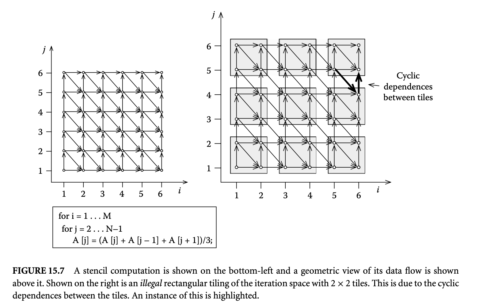 A dependence vector for an -dimensional perfect loop nest is an -vector , where the th component corresponds to the th loop (counted from outermost to innermost). A distance vector is a dependence vector , that is, every component is an integer. A dependence distance is the distance between the iteration that produces a value and the iteration that consumes a value. Distance vectors represent this information. The dependence distance vector for a value produced at iteration and consumed at a later iteration is . The stencil computation given in Figure 15.7 has three dependences. The values consumed at an iteration are produced at iterations , , and . The corresponding three dependence vectors are and .
Tiling is an iteration reordering transformation. Tiling reorders the iterations to be executed in a block-by-block or tile-by-tile fashion. Consider the tiled iteration space shown in Figure 15.7 and the following execution order. Both the tiles and the points within a tile are executed in the lexicographic order. The tiles are also executed in an atomic fashion, that is, all the iterations in a tile are executed before any iteration of another tile. It is very instructive to pause for a moment and ask whether this tiled execution order preserves all the dependences of the original computation. One can observe that the dependence is not preserved, and hence the tiling is illegal. There exists a nice geometric way of checking the legality of a tiling. A given tiling is illegal if there exist cyclic dependences between tiles. An instance of this cyclic dependence is highlighted in Figure 15.7.
The legality of tiling is determined not by the dependences alone, but also by the shape of the tiles.10 We saw (Figure 15.7) that tiling the stencil computation with rectangles is illegal. However, one might wonder whether there are other tile shapes for which tiling is legal. Yes, tiling with parallelograms is legal as shown in Figure 15.8. Note how the change in the tile shape has avoided the cyclic dependences that were present in the rectangular tiling. Instead of considering nonrectangular shapes that make tiling legal, one could also consider transforming the data dependences so that rectangular tiling becomes legal. Often, one can easily find such transformations. A commonly used transformation is skewing. The skewed iteration space is shown in Figure 15.8 together with a rectangular tiling. Compare the dependences between tiles in this tiling with those in the illegal rectangular tiling shown in Figure 15.7. One could also think of more complicated tile shapes, such as hexagons or octagons. Because of complexity of tiled code generation such tile shapes are not used.
Legality of tiling also depends on the shape of the iteration space. However, for practical applications, we can check the legality with the shape of the tiles and dependence information alone.
A given tiling can be characterized by the shape and size of the tiles, both of which can be concisely specified with a matrix. Two matrices, clustering and tiling, are used to characterize a given tiling. The clustering matrix has a straightforward geometric interpretation, and the tiling matrix is its inverse and is useful in defining legality conditions. A parallelogram (or a rectangle) has four vertices and four edges. Let us pick one of the vertices to be the origin. Now we have two edges or two vertices adjoining the origin. The shape and size of the tiles can be specified by characterizing these edges or vertices. We can easily generalize these concepts to higher dimensions. In general, an -dimensional parallelepiped has vertices and facets (higher-dimensional edges), out of which facets and vertices adjoin the origin. A clustering matrix is an square matrix whose columns correspond to the facets that determine a tile. The clustering matrix has the property that the absolute value of its determinant is equal to the tile volume.
The clustering matrices of the parallelogram and rectangular tilings shown in Figure 15.8 are

the first column represents the horizontal edge, and the second represents the oblique edge. In , the first column represents the horizontal edge, and the second represents the vertical edge.
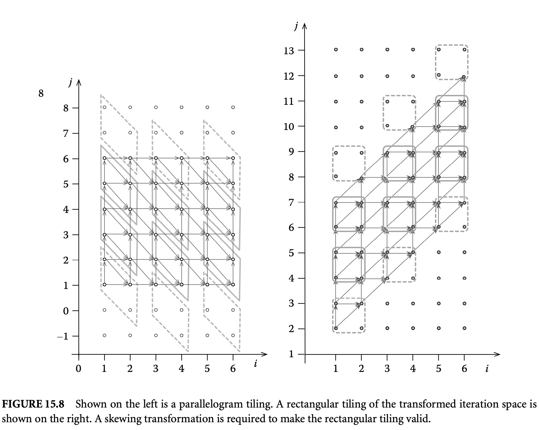
The tiling matrix is the inverse of the clustering matrix. The tiling matrices of the parallelogram and the rectangular tilings shown in Figure 15.8 are
 For rectangular tiling the edges are always along the canonical axes, and hence, there is no loss of generality in assuming that the tiling and clustering matrices are diagonal. The tiling is completely described by just the so-called tile size vector, , where each denotes the tile size along the th dimension. The clustering and tiling matrices are simply and , where denotes the diagonal matrix with as the diagonal entries.
A geometric way of checking the legality of a given tiling was discussed earlier. One can derive formal legality conditions based on the shape and size of the tiles and the dependences. Let be the set of dependence distance vectors. A vector is lexicographically nonnegative if the leading nonzero component of the is positive, that is, or both and . The floor operator when used on vectors is applied component-wise, that is, . The legality condition for a given (rectangular or parallelepiped) tiling specified by the tiling matrix and dependence set is
 The above condition formally captures the presence or absence of cycles between tiles.
We can now apply this legality condition to the stencil computation example. Let , the set of dependence vectors from the original or given stencil computation, and , the dependence vectors obtained after applying the skewing transformation to the original dependences. Earlier we showed that rectangular tiling of the original iteration space is not legal based on the existence of cycles between tiles (cf. Figure 15.7). This can also be verified by observing that the condition for validity, , is not satisfied, since, for the dependence vector in , we have . However, for the same dependences, , as shown in Figure 15.8, a parallelogram tiling is valid. This validity is confirmed by the satisfaction of the constraint . We also showed that a skewing transformation of the iteration space can make rectangular tiling valid. This can also be verified by observing the satisfaction of . In the case of rectangular tiling the legality condition can be simplified by using the fact that the tiling can be completely specified by the tile size vector . The legality condition for rectangular tiling specified by the tile size vector for a loop nest with a set of dependences is
 A rectangular tiling can also be viewed as a sequence of two transformations: strip mining and loop interchange. This view is presented by Raman and August in this text [84].
15.3.1.2 Optimal Tiling
Selecting the tile shape and selecting the sizes are two important tasks in using loop tiling. If rectangular tiling is valid or could be made valid by appropriate loop transformation, then it should be preferred over parallelepipeds. This preference is motivated by the simplicity and efficiency in tiled code generation as well as tile size selection methods. For many practical applications we can transform the loop so that rectangular tiling is valid. We discuss rectangular tiling only. Having fixed the shape of tiles to (hyper-)rectangles, we address the problem of choosing the "best" tile sizes.
Tile size selection methods vary widely depending on the purpose of tiling. For example, when tiling for multi-processor parallelism, analytical models are often used to pick the best tile sizes. However, when tiling for caches or registers, empirical search is often the best choice. Though the methods vary widely, they can be treated in the single unifying formulation of constrained optimization problems. This approach is used in the next section to formulate the optimal tile size selection problem.
Optimal Tile Size Selection ProblemThe optimal tile size selection problem involves selecting the best tile sizes from a set of valid tile sizes. What makes a tile size valid and what makes it the best can be specified in a number of ways. Constrained optimization provides this unified approach. Validity is specified with a set of constraints, and an objective function is used to pick the best tile sizes. A constrained optimization problem has the following form:

where is the variable, is the objective function, and are constraints on . The solution to such an optimization problem has two components: (a) the minimum value of over all valid and (b) a minimizer, which is a value of at which attains the minimum value.
All the optimal tile size selection problems can be formulated as a constrained optimization problem with appropriate choice of the and s. Furthermore, the structure of and s determines the techniques that can be used to solve the optimization problem. For example, consider the problem of tiling for data locality, where we seek to pick a tile size that minimizes the number of cache misses. This can be cast into an optimization problem, where the objective function is the number of misses, and the constraints are the positivity constraints on the tile sizes and possibly upper bounds on the tile sizes based on program size parameters as well as cache capacity. In the next two sections, we will present an optimization-based approach to optimal tile size selection in the context of two problems: (a) tiling for data locality and (b) tiling for parallelism. The optimization problems resulting from optimal tiling formulations can be cast into a particular form of numerical convex optimization problems called geometric programs, for which powerful and efficient tools are widely available. We first introduce this class of convex optimization problems in the next section and use them in the later sections.
15.3.1.2.2 Geometric Programs
In this section we introduce the class of numerical optimization problems called geometric programs, which will be used in later sections to formulate optimal tile size selection problems.
Let denote the vector of real, positive variables. A function is called a posynomial function of if it has the form
 where and . Note that the coefficients must be nonnegative, but the exponents can be arbitrary real numbers, including negative or fractional. When there is exactly one nonzero term in the sum, that is, and , we call a monomial function. For example, is a posynomial (but not monomial), is a monomial (and, hence, a posynomial), while is neither. Note that posynomials are closed under addition, multiplication, and nonnegative scaling. Monomials are closed under multiplication and division.
A geometric program (GP) is an optimization problem of the form
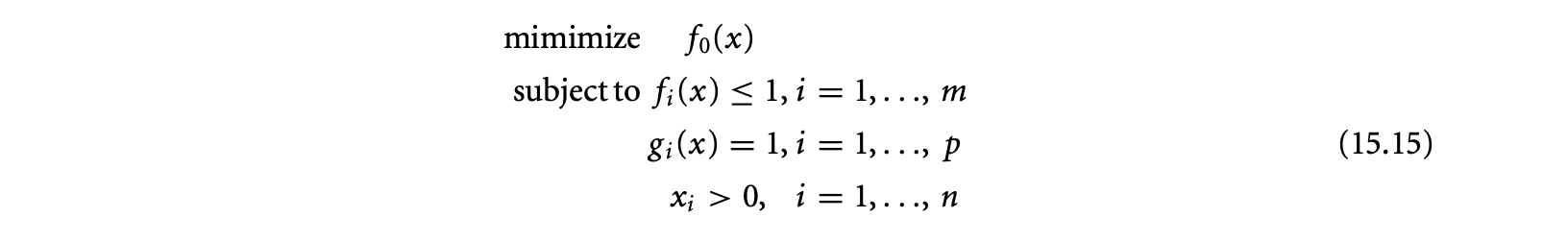
where are posynomial functions and are monomial functions. If, we call the GP an integer geometric program (IGP).
15.3.1.2.2.1 Solving IGPs
GPs can be transformed into convex optimization problems using a variable substitution and solved efficiently using polynomial time interior point methods. Integer solutions can be found by using a branch-and-bound algorithm. Tools such as YALMIP provide a high-level symbolic interface (in MATLAB) that can be used to define and solve IGPs. The number of (tile) variables of our IGPs are related to number of dimensions tiled and hence are often small. In our experience with solving IGPs related to tiling, the integer solutions were found in a few (fewer than 10) iterations of the branch-and-bound algorithm. The (wall clock) running time of this algorithm was just a few seconds, even with the overhead of using the symbolic MATLAB interface.
15.3.1.2.3 Tiling for Parallelism
We consider a distributed memory parallel machine as the execution target. Message passing is a widely used interprocess communication mechanism for such parallel machines. The cost of communication in such systems is significant. Programs with fine-grained parallelism require frequent communications and are not suited for message-passing-style parallel execution. We need to increase the granularity of parallel computation and make the communications less frequent. Tiling can be used to increase the granularity of parallelism from fine to coarse. Instead of executing individual iterations in parallel, we can execute tiles in parallel, and instead of communicating after every iteration, we communicate between tiles. The tile sizes determine how much computation is done between communications.
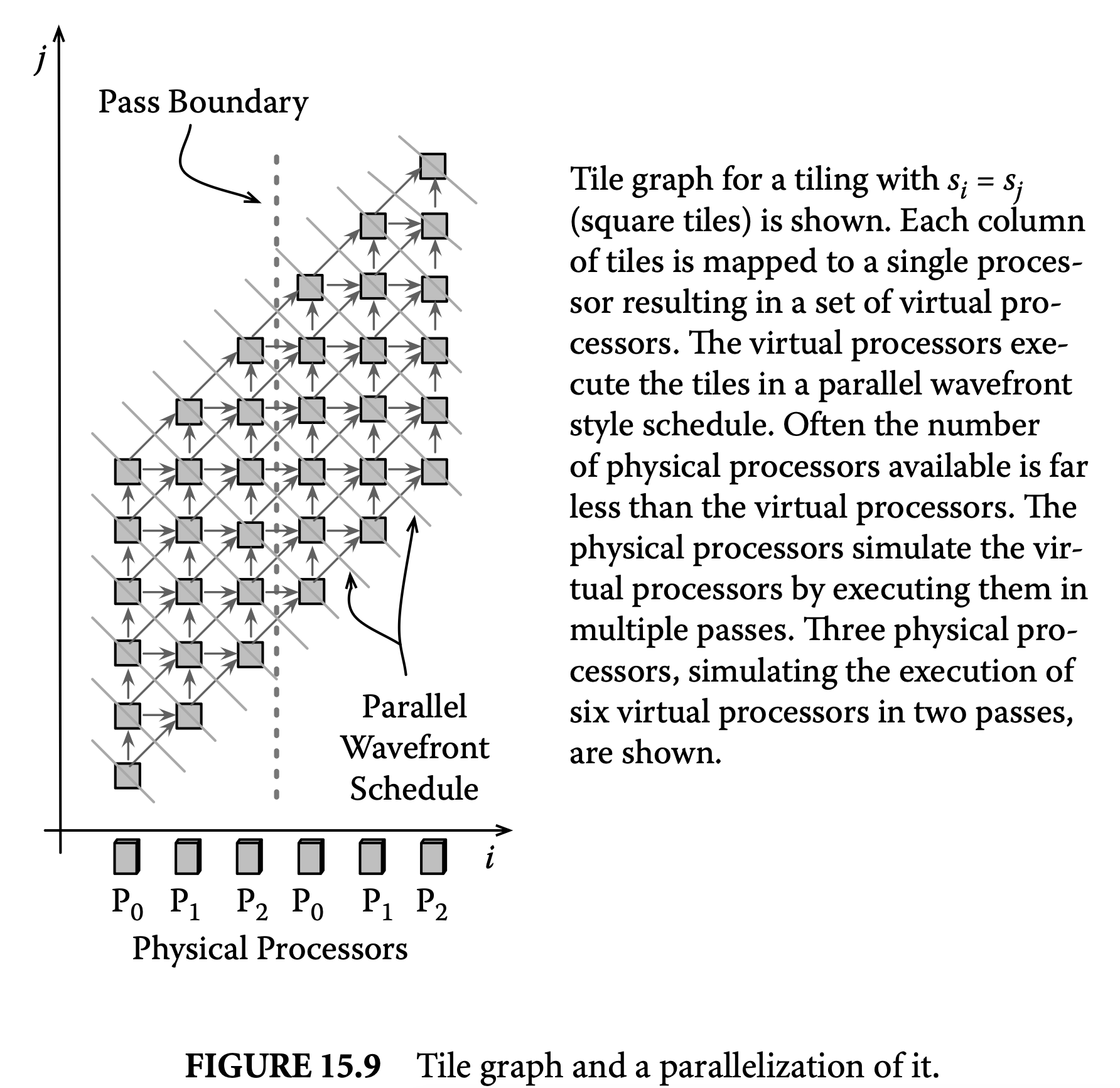
Consider the rectangular tiling shown in Figure 15.8. We seek to execute the tiles in parallel. To do this we need (a) a processor mapping that maps tiles to processors and (b) a schedule that specifies a (parallel) time stamp for each tile. A parallelization of a tiled iteration space involves derivation of a processor mapping and a schedule. A better abstraction of the tiled iteration space useful in comparing and analyzing different parallelizations is the tile graph. A tile graph consists of nodes that are tiles and edges representing dependences between them. Figure 15.9 shows the tile graph of the tiling shown in Figure 15.8. The dependences between tiles are induced by the dependences between the iterations and the tiles they are grouped into. The shape of the tile graph is determined by the shape of the tiled iteration space as well as the tile sizes. The shapes of the tile graph (Figure 15.9) and the rectangular tiled iteration space (Figure 15.8) are the same because the tile sizes are the same. It is useful to pause for a moment and think of the tile graph shape when and .
To parallelize the tile graph we need to find a parallel schedule and a processor mapping. As shown in Figure 15.9, the wavefronts corresponding to the lines define a parallel schedule -- all the tiles on a wavefront can be executed in parallel. We can verify that this schedule is valid by observing that any given tile is scheduled after all the tiles it depends on are executed. A processor mapping is valid if it does not map two tiles scheduled to execute at the same time to the same processor. There are many valid processor mappings possible for this schedule. For example, one can easily verify that the following three mappings are valid: (a) map each column of tiles to a processor, (b) map each row of tiles to a processor, and (c) map all the tiles along the diagonal line to a single processor. Though all of them are valid, they have very different properties: the first (column-wise) and the last (diagonal) map the same number of tiles to each processor, whereas the second (row-wise) maps a different number of tiles to different processors. For a load-balanced allocation one would prefer the column-wise or the diagonal mappings. However, for simplicity of the resulting parallel program, one would prefer the column-wise over the diagonal mapping.
Typically the number of processors that results from a processor mapping is far greater than the number of available processors. We call the former the virtual processors and the latter the physical processors. Fewer physical processors simulate the execution of the virtual processors in multiple passes. For example, the column-wise mapping in Figure 15.9 results in six virtual processors, and they are simulated by three physical processors in two passes. Tiles are executed in an atomic fashion; all the iterations in a tile are executed before any iteration of another tile. The parallel execution proceeds in a wavefront style.
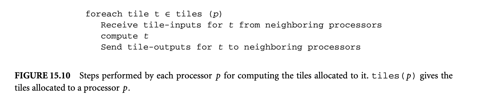 We call a parallelization idle-free if it has the property that once a processor starts execution it will never be idle until it finishes all the computations assigned to it. We call a parallelization load-balanced if it has the property that all the processors are assigned an (almost) equal amount of work. For example, the column-wise and diagonal mappings are load-balanced, whereas the row-wise mapping is not. Furthermore, within a given pass, the wavefront schedule is idle-free. Across multiple passes, it will be idle-free if by the time the first processor finishes its first column of tiles the last processor finishes at least one tile. This will be true whenever the number of tiles in a column is more than the number of physical processors.
15.3.1.2.4 An Execution Time Model
After selecting a schedule and a processor mapping, the next step is to pick the tile size. We want to pick the tile size that minimizes the execution time. We will develop an analytical model for the total running time of the parallel program and then use it to formulate a constrained optimization problem, whose solution will yield the optimal tile sizes.
We choose the wave front schedule and the column-wise processor mapping discussed earlier. Recall that the column-wise mapping is load-balanced, and within a pass the wave front schedule is idle-free. To ensure that the schedule is also idle-free across passes, we will characterize and enforce the constraint that the number of tiles in a column is greater than the number of physical processors. Furthermore, we consider the following receive-compute-send execution pattern (shown in Figure 10): every processor first receives all the inputs it needs to execute a tile and then executes the tiles and then sends the tile outputs to other processors. The total execution time is the time elapsed between the start of the first tile and the completion of the last tile. Let us assume that all the passes are full, that is, in each pass all the processors have a column of tiles to execute. Now, the last tile will be executed by the last processor, and its completion time will give the total execution time. Given that the parallelization is idle-free, the total time taken by any processor is equal to the initial latency (time it waits to get started) and the time it takes to compute all the tiles allocated to it. Hence, the sum of the latency and the computation time of the last processor is equal to the total execution time. Based on this reasoning, the total execution time is

where denotes the latency last processor to start, denotes the number of tiles allocated per processor, and is the time to execute a tile (sequentially) by a single processor. Here, the term denotes the time any processor takes to execute all the tiles allocated to it. Given that we have a load-balanced processor mapping, this term is same for all processors. In the following derivations, is the number of physical processors, and denote the size of the iteration space along and , respectively, and and are the tile sizes along and , respectively.
Let us now derive closed-form expressions for the terms discussed above. The time to execute a tile, , is the sum of the computation and communication time. The computation time is proportional to the area of the rectangular tile and is given by . The constant denotes the average time to execute one iteration. The communication time is modeled as an affine function of the message size. Every processor receives the left edge of the tile from its left neighbor and sends its right edge to the right neighbor. This results in two communications with messages of size , the length of the vertical edge of
a tile. The cost of sending a message of size is modeled by , where and are constants that denote the transmission cost per byte and the start-up cost of a communication call, respectively. The cost of the two communications performed for each tile is . The total time to execute a tile is now .
The number of tiles allocated to a processor is equal to the number of columns allocated to a processor times the number of tiles per column. The number of columns is equal to the number of passes, which is . The tiles per column is equal to , which makes .
The dependences in the tile graph induce the delay between the start of the processors. The slope , known as the rise, plays a fundamental role in determining the latency. The last processor can start as soon as the processor before it completes the execution of its first two tiles. Formally, the last processor can start its first tile only after . For example, in Figure 15.9 the last processor can start only after four time steps since and , yielding . Since at each time step a processor computes a tile, gives the time after which the last processor can start, that is, .
To ensure that there is no idle time between passes, we need to constrain the tile sizes such that by the time the first processor finishes its column of tiles, the last processor must have finished its first tile. The time the first processor takes to complete a column of tiles is equal to , and the time by which the last processor would finish its first tile is . The no idle time between passes constraint is .
Using the terms derived above we can now formulate an optimization problem to pick the optimal tile size.
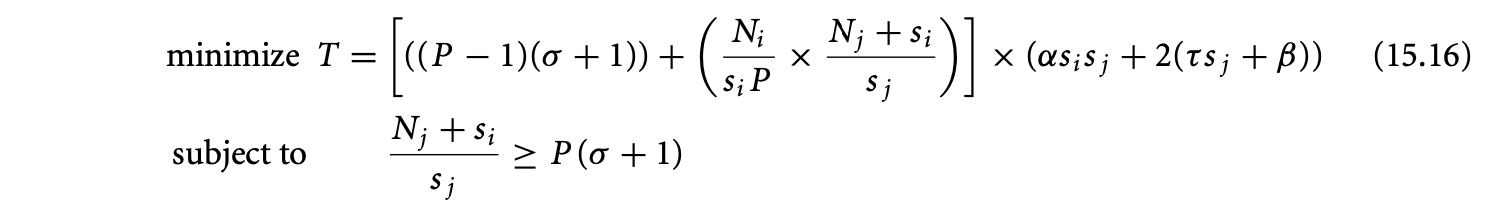 The solution to the above optimization problem yields the optimal tile sizes, that is, the tile sizes that minimize the total execution time of the parallel program, subject to the constraint that there is no idle time between passes.
The optimization problem in Equation 15.16 can be transformed into a GP. The objective function is directly a posynomial. With the approximation of , the constraint transforms into

which is the required form for a GP constraint. Adding to it the obvious constraints that tile sizes are integers and positive, that is, , and , we get an IGP that can be solved efficiently as discussed above. The solution to this IGP will yield the optimal tile sizes.
15.3.1.2.4.1 Generality of Approach
The analysis techniques presented above can be directly extended to higher-dimensional rectangular or parallelepiped iteration spaces. For example, stencil computations with two-dimensional or three-dimensional data grids, after skewing to make rectangular tiling valid, have parallelepiped iteration spaces, and the techniques described above can be directly applied to them. The GP-based modeling approach is quite general. Because of the fundamental positivity property of tile sizes, often the functions used in modeling parallel execution time or communication or computation volumes are posynomials. This naturally leads to optimization problems that are GPs.
15.3.1.2.5 Tiling for Data Locality
Consider the stencil computation shown in Figure 15.7. Every value, , computed at an iteration is used by three other computations as illustrated in the geometric view shown in Figure 15.7 (left).
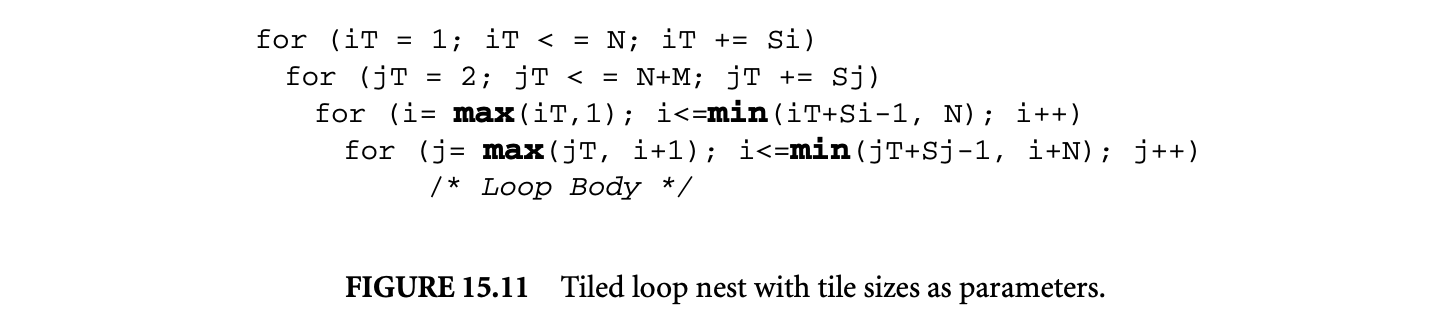 The three uses are in iterations and . Consider the case when the size of A is much larger than the cache size. On the first use at iteration , the value will be cache. However, for the other two uses, and , the value may not be in cache, resulting in a cache miss. This cache miss can be avoided if we can keep the computed values in the cache until their last use. One way to achieve this is by changing the order of the computations such that the iterations that use a value are computed "as soon as" the value itself is computed. Tiling is widely used to achieve such reorderings that improve data locality. Furthermore, the question of how soon the iterations that use a value should be computed is dependent on the size of the cache and processor architecture. This aspect can be captured by appropriately picking the tile sizes.
Consider the rectangular tiling of the skewed iteration space shown in Figure 15.8 (right). Figure 15.11 shows the tiled loop nest of the skewed iteration space, with tile sizes as parameters. The new execution order after tiling is as follows: both the tiles and the points within a tile are executed in column-major order. Observe how the new execution order brings the consumers of a value closer to the producer, thereby decreasing the chances of a cache miss. Figure 15.8 (right) shows a tiling with tiles of sizes . In general, the sizes are picked so that the volume data touched by a tile, known as its footprint, fits in the cache, and some metric such as number of misses or total execution time is minimized. A discussion of other loop transformations (e.g., loop fusion, fission, etc.) aimed at memory hierarchy optimization can be found in the chapter by Raman and August [84] in the same text.
15.3.1.2.5.1 Tile Size Selection Approaches
A straightforward approach for picking the best tile size is empirical search. The tiled loop nest is executed for a range of tile sizes, and the one that has the minimum execution time is selected. This search method has the advantage of being accurate, that is, the minimum execution time tile is the best for the machine on which it is obtained. However, such a search may not be feasible because of the huge space of tile sizes that needs to be explored. Often, some heuristic model is used to narrow down this space. In spite of the disadvantages, such an empirical search is the popular and widely used approach for picking the best tile sizes. For the obvious reason of huge search time, such an approach is not suitable for a compiler.
Compilers trade off accuracy for search time required to find the best tile size. They use approximate cache behavior models and high-level execution time models. Efficiency is achieved by specializing the tile size search algorithm to the chosen cache and execution time models. However, such specialization of search algorithms makes it difficult to change or refine the models.
Designing a good model for the cache behavior of loop programs is hard, but even harder is the task of designing a model that would keep up with the advancements in processor and cache architectures. Thus, cache models used by compilers are often outdated and inaccurate. In fact, the performance of a tiled loop nest generated by a state-of-the-art optimizing compiler could be a few factors poorer than the one hand-tuned with an empirical search for best tile sizes. This has led to the development of the so-called auto-tuners, which automatically generate loop kernels that are highly tuned to a given architecture. Tile sizes are an important parameter tuned by auto-tuners. They use a model-driven empirical search to pick the tile sizes. Essentially they do an empirical search for the best tile size over a space of tile sizes and use an approximate model to prune the search space.
15.3.1.2.5.2 Constrained Optimization Approach
Instead of discussing specialized algorithms, we present a GP-based framework that can be used to develop models, formulate optimal tile size selection problems, and obtain the best tile sizes by using the efficient numerical solvers. We illustrate the use of the GP framework by developing an execution time model for the tiled stencil computation and formulating a GP whose solution will yield the optimal tile sizes. Though we restrict our discussion to this illustration-based presentation, the GP framework is quite general and can be used with several other models. For example, the models used in the IBM production compiler or the one used by the auto-tuner ATLAS can be transformed into the GP framework.
The generality and wide applicability of the GP framework stems from a fundamental property of the models used for optimal tile size selection. The key property is based on the following: tile sizes are always positive and all these models use metrics and constraints that are functions of the tile sizes. These functions of tile size variables often turn out to be posynomials. Furthermore, the closure properties of posynomials provide the ability to compose models. We illustrate these in the following sections.
15.3.1.2.5.3 An Analytical Model
We will first derive closed-form characterizations of several basic components related to the execution of a tiled loop and then use them to develop an analytical model for the total execution time. We will use the following parameters in the modeling. Some of them are features of processor memory hierarchy and others are a combination of processor and loop body features:
- : The average cost (in cycles) of computing an iteration assuming that the accessed data values are in the lowest level of cache. This can be determined by executing the loop for a small number of iterations, such that the data arrays fit in the cache, and taking the average.
- : The cost (in cycles) for moving a word from main memory to the lowest level of cache. This can be determined by the miss penalties associated with caches, translation look aside buffers, and so on.
- : The average cost (in cycles) to compute and check loop bounds. This can be determined by executing the loops without any body and taking the average.
- and : The capacity and line size, in words, of the lowest level of cache. These two can be directly determined from the architecture manual.
15.3.1.2.5.4 Computation Cost
The number of iterations computed by a tile is given by the tile area . If the data values are present in the lowest level of cache, then the cost of computing the iterations of a tile, denoted by , is , where is the average cost to compute an iteration.
15.3.1.2.5.5 Loop Overhead Cost
Tiling (all the loops of) a loop nest of depth results in loops of which the outer loops enumerate the tiles and the inner loops enumerate points in a tile. We refer to the cost for computing and testing loop bounds as the loop overhead cost. In general, the loop overhead is significant for tiled loops and needs to be accounted for in modeling the execution time. The loop overhead cost of a given loop is proportional to the number of iterations it enumerates. In general, , the loops bounds check cost, is dependent on the complexity of the loop bounds of a given loop. However, for notational and modeling simplicity we will use the same for all the loops. Now the product of with the number iterations of a loop gives the loop overhead of that loop.
Consider the tiled loop nest of the skewed iteration space shown in Figure 15.11. The total number of iterations enumerated by the tile-loops (iT and jT loops) is . The loop overhead of the tile-loops is . With the small overapproximation of partial tiles by full tiles, the number of iterations enumerated by the point-loops (i and j loops), for any given iteration of the outer tile-loops,is . The loop overhead of the point-loops is . The total loop overhead of the tiled loop nest is denoted by .
15.3.1.2.5.6 Footprint of a Tile
The footprint of a tile is the number of distinct array elements touched by a tile. Let us denote the footprint of a tile of size s by F(s). Deriving closed-form descriptions of F(s) for loop nests with an arbitrary loop body is hard. However, for the case when the loop body consists of references to arrays and the dependences are distance vectors, we can derive closed-form descriptions of F(s). However, for the case when the loop body contains affine references, deriving closed-form expressions for F(s) is complicated. We illustrate the steps involved in deriving F(s) for dependence distance vectors with our stencil computation example.
Consider the tiled stencil computation. Let s= be the tile size vector, where represents the tile size along i and along j. Each (nonboundary, full) tile executes iterations updating the values of the one-dimensional array A. The number of distinct values of A touched by a tile is proportional to one of its edges, namely, . One might have to store some intermediate values during the tiled execution, and these require an additional array of size . Adding these two together, we get . Note that F(s) takes into account the reuse of values. Loops with good data locality (i.e., with at least one dimension of reuse) have the following property: the footprint is proportional to the (weighted) sum of the facets of the tile. Note that our stencil computation has this property, and hence F(s) is the sum of the facets (here just edges) and . To maximize the benefits of data locality, we should make sure that the footprint F(s) fits in the cache.
15.3.1.2.5.7 Load Store Cost of a Tile
Earlier during the calculation of the computation cost, we assumed that the values are available in the lowest level of the cache. Now we will model the cost of moving the values between main memory and the lowest level of cache. To derive this cost we need a model of the cache. We will assume a fully associative cache of capacity C words with cache lines of size L words. is the cost of getting a word from the main memory to the cache. Ignoring the reuse of cache lines across tiles, F(s) provides a good estimated number of values accessed by a tile during its execution. Let be the number of cache lines needed for F(s). We have , where L is the cache line size. Then the load store cost of a tile, denoted by , is
15.3.1.2.5.8 Total Execution Time of a Tiled Loop Nest
The total execution time of the tiled loop nest is the sum of the time it takes to execute the tiles and the loop overhead. The time to execute the tiles can be modeled as the product of time to execute a tile times the number of tiles. For our stencil computation the iteration space is a parallelogram, and calculating the number of rectangles that cover it is a hard problem. However, we can use the reasonable approximation of to model the number of tiles, denoted by ntiles (s). The total execution time T is given by
 where ntiles (s) is the number of tiles, is the cost of executing a tile, is the load store cost, and is the loop overhead.
15.3.1.2.5.9 Optimal Tile Size Selection Problem Formulation
Using the quantities derived above, we can now formulate an optimization problem whose solution will yield the optimal tile size - one that minimizes the total execution time. Recall that the function T (Equation 15.17) derived above models the execution time under the assumption that the data accessed by a tile fits in the cache. We model this assumption by translating it into a constraint in the optimization problem. Recall that F(s) measures the data accessed by a tile, and gives the number of cache lines needed for F(s). The constraint , where C is the cache capacity, ensures that all the data touched by a tile fits in the cache. Now we can formulate the optimization problem to find the tile size that minimizes as follows:
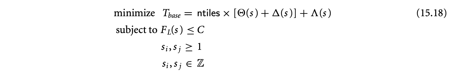 where the last two constraints ensure that and are positive and are integers.
15.3.1.2.5.10 Optimal Tiling Problem Is an IGP
The constrained optimization problem formulated above (Equation 15.18) can be directly cast into an IGP (integer geometric program) of the form of Equation 15.15. The constraints are already in the required form. The objective function is a posynomial. This can be easily verified by observing that the terms used in the construction of , namely, , and , are all posynomials, and posynomials are closed under addition -- the sum of posynomials is a posynomial. Based on the above reasoning, the optimization problem Equation 15.18 is an IGP.
15.3.1.2.5.11 A Sophisticated Execution Time Model
One can also consider a sophisticated execution time model that captures several hardware and compiler optimizations. For example, modern processor architectures support nonblocking caches, out-of-order issue, hardware prefetching, and so on, and compilers can also do latency hiding optimizations such as software prefetching and instruction reordering. As a result of these hardware and compiler optimizations, one can almost completely hide the load-store cost. In such a case, the cost of a tile is not the sum of the computation and communication cost, but the maximum of them. We model this sophisticated execution time with the function as follows:

Thanks to our unified view of the optimization problem approach, we can substitute with in the optimization problem Equation 15.18 and solve for the optimal tile sizes. However, must be a posynomial for this substitution to yield a GP. We can easily transform to a posynomial by introducing new variables to eliminate the operator.
15.3.1.3 Tiled Code Generation
An important step in applying the tiling transformation is the generation of the tiled code. This step involves generation of tiled loops and the transformed loop body. Since tiling can be used for a variety of purposes, depending on the purpose, the loop body generation can be simple and straightforward to complicated. For example, loop body generation is simple when tiling is used to improve data cache locality, whereas, in the context of register tiling, loop body generation involves loop unrolling followed by scalar replacement, and in the context of tiling for parallelism, loop body generation involves generation of communication and synchronization. There exist a variety of techniques for loop body generation, and a discussion of them is beyond the scope of this article. We will present techniques that can be used for tiled loop generation both when the tile sizes are fixed and when they are left as symbolic parameters.
15.3.1.3 Tiled Loop Generation
We will first introduce the structure of tiled loops and develop an intuition for the concepts involved in generating them. Consider the iteration space of a two-dimensional parallelogram such as the one shown in Figure 15.12, which is the skewed version of the stencil computation. Figure 15.13 shows a geometric view of the iteration space superimposed with a rectangular tiling. There are three types of tiles: full (which are completely contained in the iteration space), partial (which are not completely contained but have a nonempty intersection with the iteration space), and empty (which do not intersect the iteration space).
 The lexicographically earliest point in a tile is called its origin. The goal is to generate a set of loops that scans (i.e., visits) each integer point in the original iteration space based on the tiling transformation, where the tiles are visited lexicographically and then the points within each tile are visited lexicographically. We can view the four loops that scan the tiled iteration space as two sets of two loops each, where the first set of two loops enumerate the tile origins and the next set of two loops visit every point within a tile. We call the loops that enumerate the tile origins the tile-loops and those that enumerate the points within a tile the point-loops.
15.3.1.3.2 Bounding Box Method
One solution for generating the tile-loops is to have them enumerate every tile origin in the bounding box of the iteration space and push the responsibility of checking whether a tile contains a valid iteration to the point-loops. The tiled loop nest generated with this bounding box scheme is shown in Figure 15.11. The first two loops (iT and jT) enumerate all the tile origins in the bounding box of size , and the two inner loops (i and j) scan the points within a tile. A closer look at the point-loop bounds reveals its simple structure. One set of bounds is from what we refer to as the tile box bounds, which restrict the loop variable to points within a tile. The other set of bounds restricts the loop variable to points within
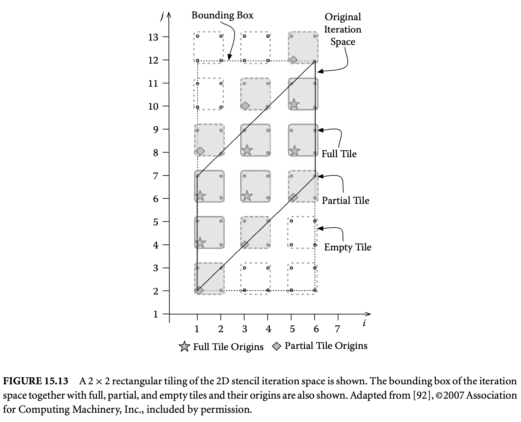
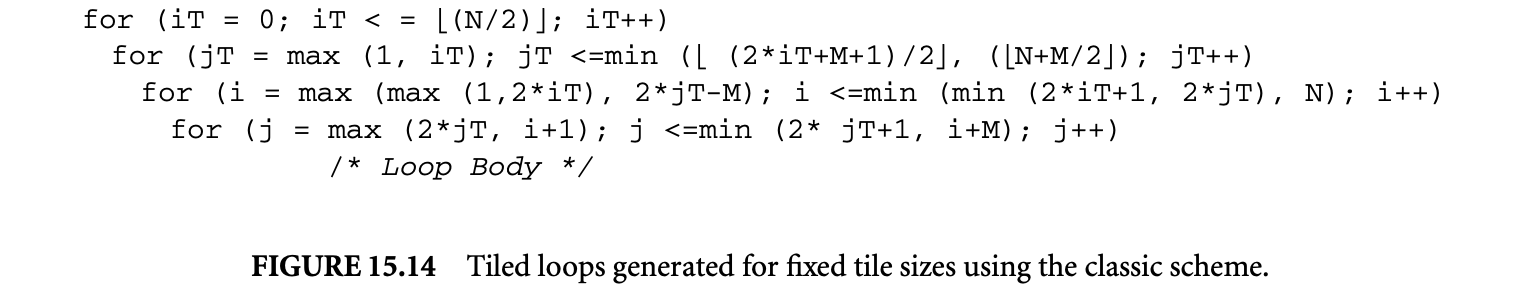
the iteration space. Combining these two sets of bounds, we get the point-loops that scan points within the iteration space and tiles. Geometrically, the point-loop bounds correspond to the intersection of the tile box (or rectangle) and the iteration space, here the parallelogram in Figure 15.13.
The bounding box scheme provides a couple of important insights into the tiled-loop generation problem. First, the problem can be decomposed into the generation of tile-loops and the generation of point-loops. Such a decomposition leads to efficient loop generation, since the time and space complexity of loop generation techniques is a doubly exponential function of the number of bounds. The second insight is the scheme of combining the tile box bounds and iteration space bounds to generate point-loops. An important feature of the bounding box scheme is that tile sizes need not be fixed at loop generation time, but can be left as symbolic parameters. This feature enables generation of parameterized tiled loops, which is useful in iterative compilation, auto-tuners, and runtime tile size adaptation. However, the empty tiles enumerated by tile-loops can become a source of inefficiency, particularly for small tile sizes.
15.3.1.3.3 When Tile Sizes Are Fixed
When the tile sizes can be fixed at the loop generation time, an exact tiled loop nest can be generated. The tile-loops are exact in the sense that they do not enumerate any empty tile origins. When the tile sizes are fixed, the tiled iteration space can be described as a set of linear constraints. Tools such as OMEGA and CLOOG provide standard techniques to generate loops that scan the integer points in sets described by linear constraints. These tools can be used to generate the tiled loop nest. The exact tiled loop nest for the two-dimensional stencil example is shown in Figure 15.14. Note that the efficiency due to the exactness of the tile-loops has come at the cost of fixing the tile sizes at generation time. Such loops are called fixed tiled loops.
The classic schemes for tiled loop generation take as input all the constraints that describe the bounds of the loops of the tiled iteration space, where is the depth of the original loop nest. Since the time-space complexity of the method is doubly exponential on the number of constraints, an increase in the number (from to ) of constraints might lead to situations where the loop generation time becomes prohibitively expensive. Similar to the bounding box technique, tiled loop generation for fixed tile sizes can also be decomposed into generating tile-loops and point-loops separately. Such a decomposition will reduce the number of constraints considered into each step by half and will improve the scalability of the tiled loop generation method.
15.3.2 Tiling Irregular Applications
Applications that make heavy use of sparse data structures are difficult to parallelize and reschedule for improved data locality. Examples of such applications include mesh-quality optimization, nonlinear equation solvers, linear equation solvers, finite element analysis, N-body problems, and molecular dynamics simulations. Sparse data structures introduce irregular memory references in the form of indirect array accesses (e.g., A[B[i]]), which inhibit compile-time, performance-improving transformations such as tiling. For example, in Figure 15.15, the array A is referenced with two different indirect array accesses, p[i] and q[i].
The flow, memory-based data dependences within the loop in Figure 15.15 can be described with the dependence relation (), where iteration depends on the value generated in iteration .


The uninterpreted functions and are static place holders for quantities that are unknown until runtime. It is not possible to parallelize or tile the loop in Figure 15.15 without moving some of the required analysis to the runtime.
To address this problem, inspector and executor strategies have been developed where the inspector dynamically analyzes memory reference patterns and reorganizes computation and data, and the executor executes the irregular computation in a different order to improve data locality or exploit parallelism. The ideal role for the compiler in applying inspector and executor strategies is performing program analysis to determine where such techniques are applicable and inserting inspector code and transforming the original code to form the executor. This section summarizes how inspector and executor strategies are currently applied to various loop patterns. The section culminates with the description of a technique called full sparse tiling being applied to irregular Gauss-Seidel.
15.3.2.1 Terminology
Irregular memory references are those that cannot be described with a closed-form, static function. Irregular array references often occur as a result of indirect array references where an access to an index array is used to reference a data array (e.g., A[p[i]] and A[q[i]] in Figure 15.15). A data array is an array that holds data for the computation. An index array is an array of integers, where the integers indicate indices into a data array or another index array.
This section assumes that data dependence analysis has been performed on the loops under consideration. The dependences are represented as relations between integer tuples with contraints specified using Presburger arithmetic including uninterpreted function symbols. Presburger arithmetic includes the universal operator , existential operator , conjunction , disjunction , negation , integer addition , and multiplication by a constant.
The dependence relations are divided into flow dependences, anti dependences, and output dependences. Flow dependence relations are specified as a set of iteration pairs where the iteration in which a read occurs depends on the iteration where a write occurs. The flow dependence relation for Figure 15.15 is as follows:

An anti dependence is when a write must happen after a read because of variable reuse. The anti dependence relation for the example in Figure 15.15 is
 An output dependence is a dependence between two writes to the same memory location. The output dependence relation for the example in Figure 15.15 is

A reduction loop has no loop-carried dependences except for statements of the form
 where X is a reference to a scalar or an array that is the same on the left- and right-hand side of the assignment, there are no references to the variable being referenced by X in the expression on the right-hand side, and op is an associative operator (e.g., addition, max, min). Since associative statements
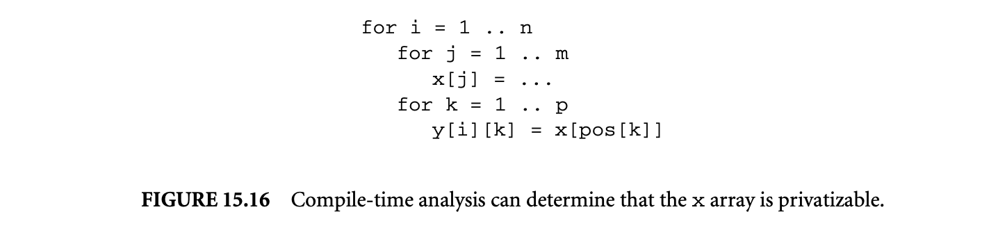 may be executed in any order, the loop may be parallelized as long as accesses to X are surrounded with a lock.
15.3.2.2 Detecting Parallelism
In some situations, static analysis algorithms are capable of detecting when array privatization and loop parallelization are possible in loops involving indirect array accesses. Figure 15.16 shows an example where compile-time program analysis can determine that the array x can be privatized, and therefore the i loop can be parallelized. The approach is to analyze the possible range of values that pos[k] might have and verify that it is a subset of the range [l..m], which is the portion of x being defined in the j loop.
If compile-time parallelism detection is not possible, then it is sometimes possible to detect parallelism at runtime. Figures 15.17 and 15.19 show loops where runtime tests might prove that the loop is in fact parallelizable. For the example in Figure 15.17, there are possible sets of flow and anti dependences between the write to A[p[i]] and the read of A[i]. If a runtime inspector determines that for all , is greater than , then the loop is parallelizable. Figure 15.18 shows an inspector that implements the runtime check and an executor that selects between the original loop and a parallel version of the loop.
To show an overall performance improvement, the overhead of the runtime inspector must be amortized over multiple executions of the loop. Therefore, one underlying assumption is that an outer loop encloses the loop to be parallelized. Another assumption needed for correctness is that the indirection arrays p and q are not modified within the loops. Figure 15.19 has an example where the inspection required might be overly cumbersome. In Figure 15.19, there are possible sets of flow and anti dependences between the write to A[p[i]] and the read of A[q[i]]. If it can be shown that for all and such that , is not equal to , then there are no dependences in the loop. Notice in Figure 15.20 that for this example, the inspector that determines whether there is a dependence requires time, thus making it quite difficult to amortize such parallelization detection for this example.
15.3.2.3 Runtime Reordering for Data Locality and Parallelism
Many runtime data reordering and iteration reordering heuristics for loops with no dependences or only reduction dependences have been developed. Such runtime reordering transformations inspect data mappings (the mapping of iterations to data) to determine the best data and iteration reordering within a parallelizable loop.
In molecular dynamics simulations there is typically a list of interactions between molecules, and each interaction is visited to modify the position, velocity, and acceleration of each molecule. Figure 15.21 outlines the main loop within the molecular dynamics benchmark moldyn. An outer time-stepping loop makes amortization of inspector overhead possible. The j loop calculates the forces on the molecules using the left and right index arrays, which indicate interaction pairs. In the j loop are two reduction
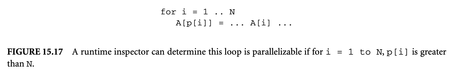
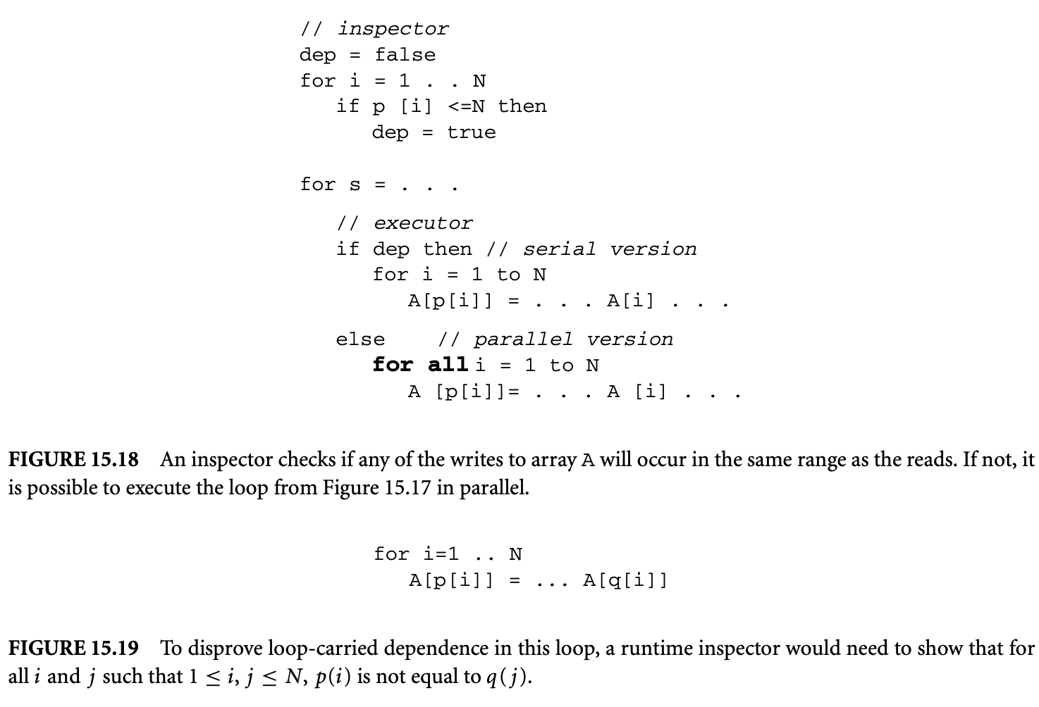
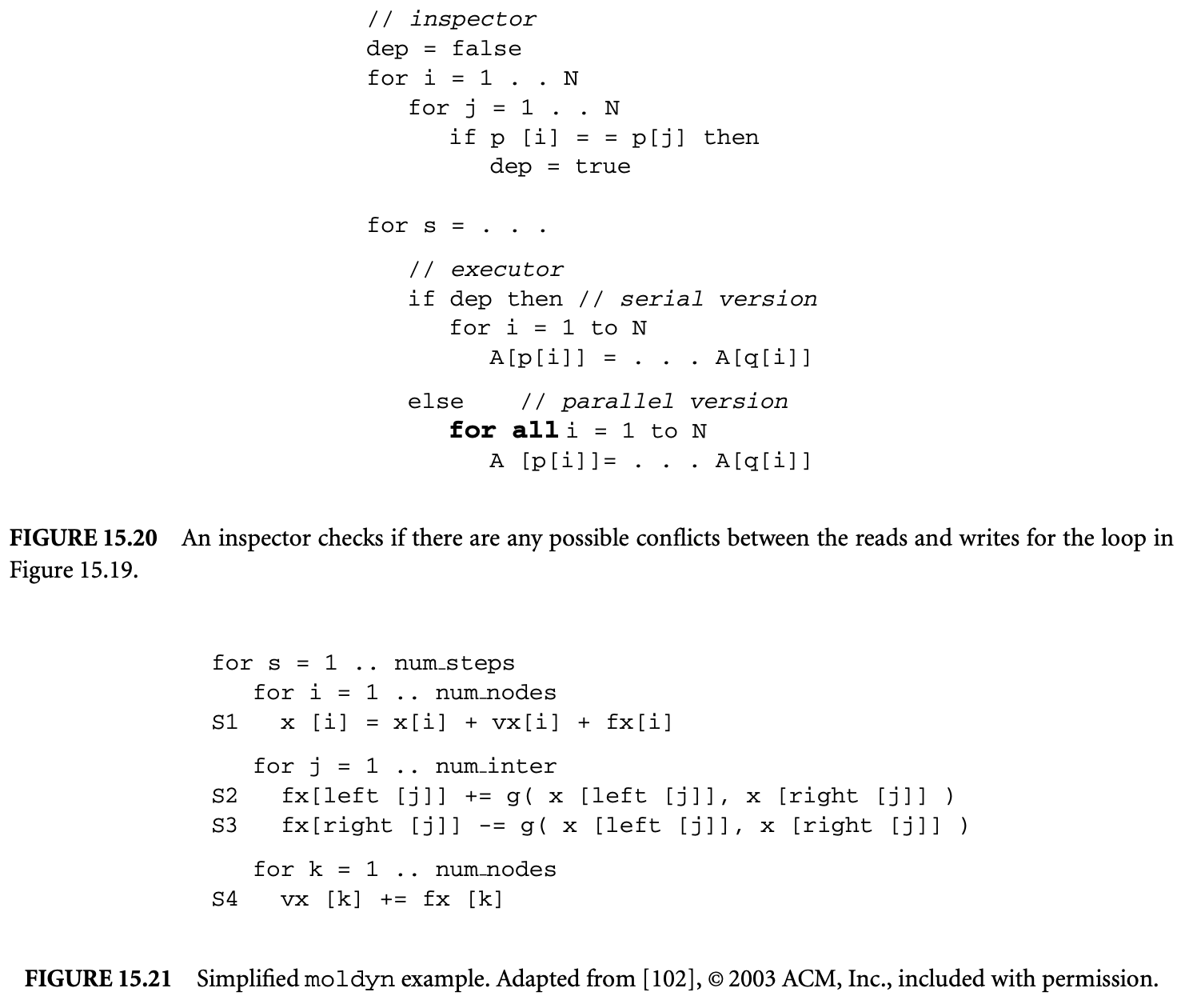
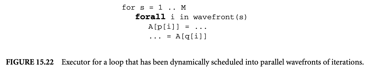
statements where the x-coordinate of the force fx for a molecule is updated as a function of the original x position for that molecule and the x position of some neighboring molecule right[i]. The j loop indirectly accesses the data arrays x and fx with the index arrays left and right.
Runtime data and iteration reorderings are legal for the j loop, because it only involves loop-carried dependences due to reductions. The data and iteration reordering inspectors can be inserted before the s loop, because the index arrays left and right are not modified within s (in some implementations of moldyn the index arrays are modified every 10 to 20 iterations, at which point the reorderings would need to be updated as well). The inspector can use various heuristics to inspect the index arrays and reorder the data arrays x and fx including: packing data items in the order they will be accessed in the loop, ordering data items based on graph partitioning, and sorting iterations based on the indices of the data items accessed. As part of the data reordering, the index arrays should be updated using a technique called pointer update. Iteration reordering is implemented through a reordering of the entries in the index array. Of course in this example, the left and right arrays must be reordered identically since entries left[i] and right[i] indicate an interacting pair of molecules. The executor is the original computation, which uses the reordered data and index arrays.
A significant amount of work has been done to parallelize irregular reduction loops on distributed memory machines. The data and computations are distributed among the processors in some fashion. Often the data is distributed using graph partitioning, where the graph arises from a physical mesh or list of interactions between entities. A common way to distribute the computations is called "owner computes," where all updates to a data element are performed by the processor where the data is allocated. Inspector and executor strategies were originally developed to determine a communication schedule for each processor so that data that is read in the loop is gathered before executing the loop, and at the end of the loop results that other processors will need in the next iteration are scattered. In iterative computations, an owner-computes approach typically involves communication between processors with neighboring data at each outermost iteration of the computation. The inspector must be inserted into the code after the index arrays have been initialized, but preferably outside of a loop enclosing the target loop. The executor is the original loop with gather and scatter sections inserted before and after.
For irregular loops with loop-carried dependences, an inspector must determine the dependences at runtime before rescheduling the loop. The goal is to dynamically schedule iterations into wavefronts such that all of the iterations within one wavefront may be executed in parallel. As an example, consider the loop in Figure 15.15. The flow, anti, and output dependences for the loop are given in Section 15.3.2.1. An inspector for detecting partial parallelism inspects all the dependences for a loop and places iterations into wavefronts. The original loop is transformed into an executor similar to the one in Figure 15.22, where the newly inserted s loop iterates over wavefronts, and all iterations within a wavefront can be executed in parallel.
15.3.2.4 Tiling Irregular Loops with Dependences11
Parts of this section are adapted from [102], ©ACM, Inc., included with permission, and from [101], with kind permission of Springer Science and Business Media © 2002.
The partial parallelism techniques described in Section 15.3.2.3 dynamically discover fine-grained parallelism within a loop. Sparse tiling techniques can dynamically schedule between loops or across outermost loops and can create course-grain parallel schedules. Two application domains where sparse tiling techniques have been found useful are iterative computations over interaction lists (e.g., molecular dynamics simulations) and iterative computations over sparse matrices. This section describes full sparse tiling, which
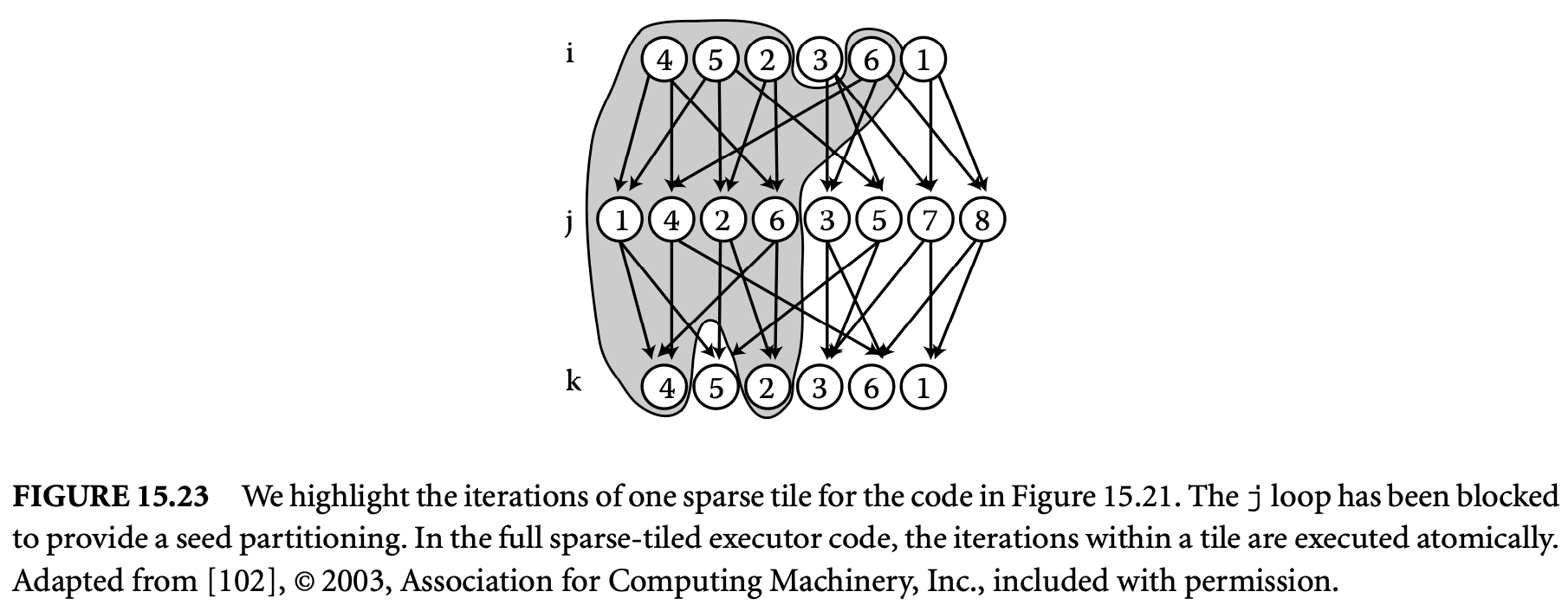 has been used to tile sparse computations across loops in a molecular dynamics benchmark and across the outermost loop of iterative computations.
15.3.2.4.1 Full Sparse Tiling for Molecular Dynamics Simulations
The runtime data and iteration reordering transformations described in Section 15.3.2 may be applied to the loop in the molecular dynamics code shown in Figure 15.21. Reordering the data and iterations within the loop is legal since the loop is a reduction. Full sparse tiling is capable of scheduling subsets of iterations across the , , and loops in the same example. The full sparse tiling inspector starts with a seed partitioning of iterations in one of the loops (or in one iteration of an outer loop). If other data and iteration reordering transformations have been applied to the loop being partitioned, then consecutive iterations in the loop have good locality, and a simple block partitioning of the iterations is sufficient to obtain an effective seed partitioning. Tiles are grown from the seed partitioning to the other loops involved in the sparse tiling by a traversal of the data dependences between loops (or between iterations of an outer loop). Growing from the seed partition to an earlier loop entails including in the tile all iterations in the previous loop that are sources for data dependences ending in the current seed partition and that have not yet been placed in a tile. Growth to a later loop is limited to iterations in the later loop whose dependences have been satisfied by the current seed partition and any previously scheduled tiles.
For the simplified example, Figure 15.23 shows one possible instance of the data dependences between iterations of the , , and loops after applying various data and iteration reorderings to each of the loops. A full sparse tiling iteration reordering causes subsets of all three loops to be executed atomically as sparse tiles. Figure 15.23 highlights one such sparse tile where the loop has been blocked to create a seed partitioning. The highlighted iterations that make up the first tile execute in the following order: iterations 4, 5, 2, and 6 in loop ; iterations 1, 4, 2, and 6 in loop ; and iterations 4 and 2 in loop . The second tile executes the remaining iterations. Figure 15.24 shows the executor that maintains the outer loop over time steps, iterates over tiles, and then within the , , and loops executes the iterations belonging
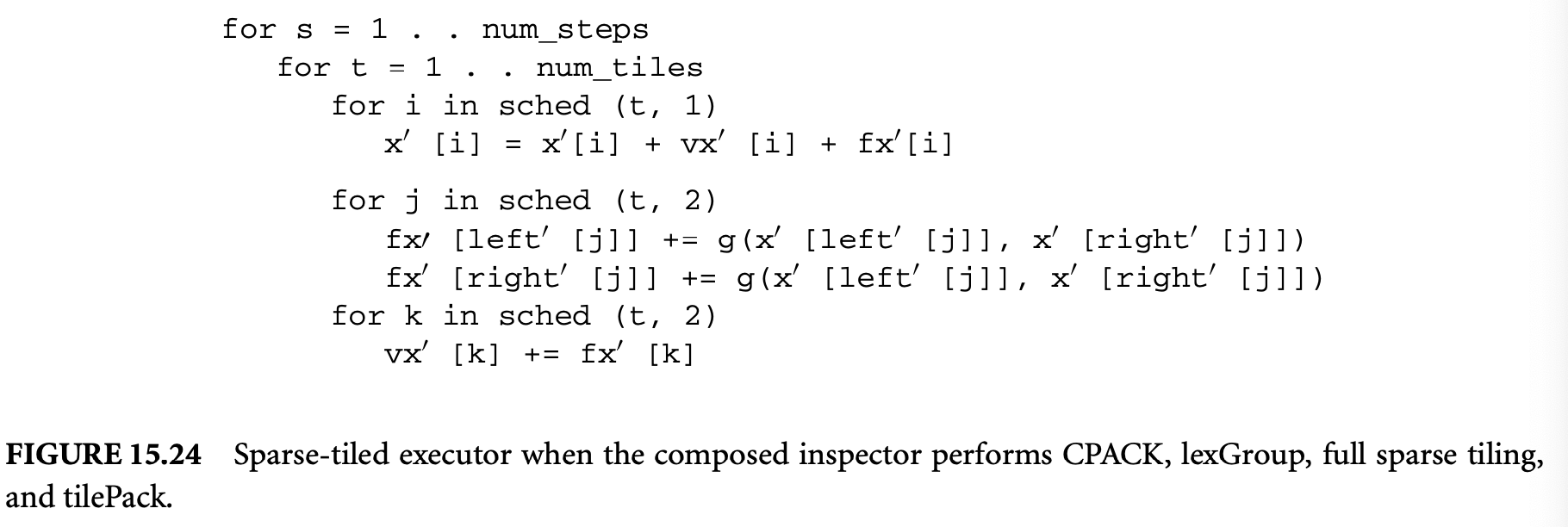
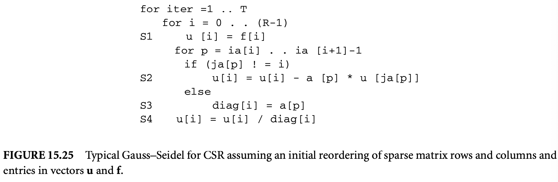
to each tile as specified by the schedule data structure. Since iterations within all three loops touch the same or adjacent data locations, locality between the loops is improved in the new schedule.
Full sparse tiling can dynamically parallelize irregular loops by executing the directed, acyclic dependence graph between the sparse tiles in parallel using a master-worker strategy. The small example shown in Figure 15.23 only contains two tiles, where one tile must be executed before the other to satisfy dependences between the , , and loops. In a typical computation where the seed partitions are ordered via a graph coloring, more parallelism between tiles is possible.
15.3.2.4.2 Full Sparse Tiling for Iterative Computations Over Sparse Matrices
Full Sparse tiling can also be used to improve the temporal locality and parallelize the Gauss-Seidel computation. Gauss-Seidel is an iterative computation commonly used alone or as a smoother within multigrid methods for solving systems of linear equations of the form , where is a matrix, is a vector of unknowns, and is a known right-hand side. Figure 15.25 contains a linear Gauss-Seidel computation written for the compressed sparse row (CSR) sparse matrix format. We refer to iterations of the outer loop as convergence iterations. The iteration space graph in Figure 15.26 visually represents an instance of the linear Gauss-Seidel computation. Each iteration point in the iteration space represents all the computation for the unknown at convergence iteration (one instance of S1 and S4 and multiple instances of S2 and S3). The iter axis shows three convergence iterations. The dark arrows show the data dependences between iteration points for one unknown in the three convergence iterations. The unknowns are indexed by a single variable , but the computations are displayed in a two-dimensional plane parallel to the and axes to exhibit the relationships between iterations. At each convergence iteration the relationships between the unknowns are shown by the lightly shaded matrix graph. Specifically, for each nonzero in the sparse matrix , , there is an edge in the matrix graph. The original
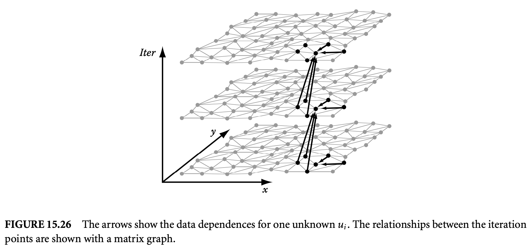
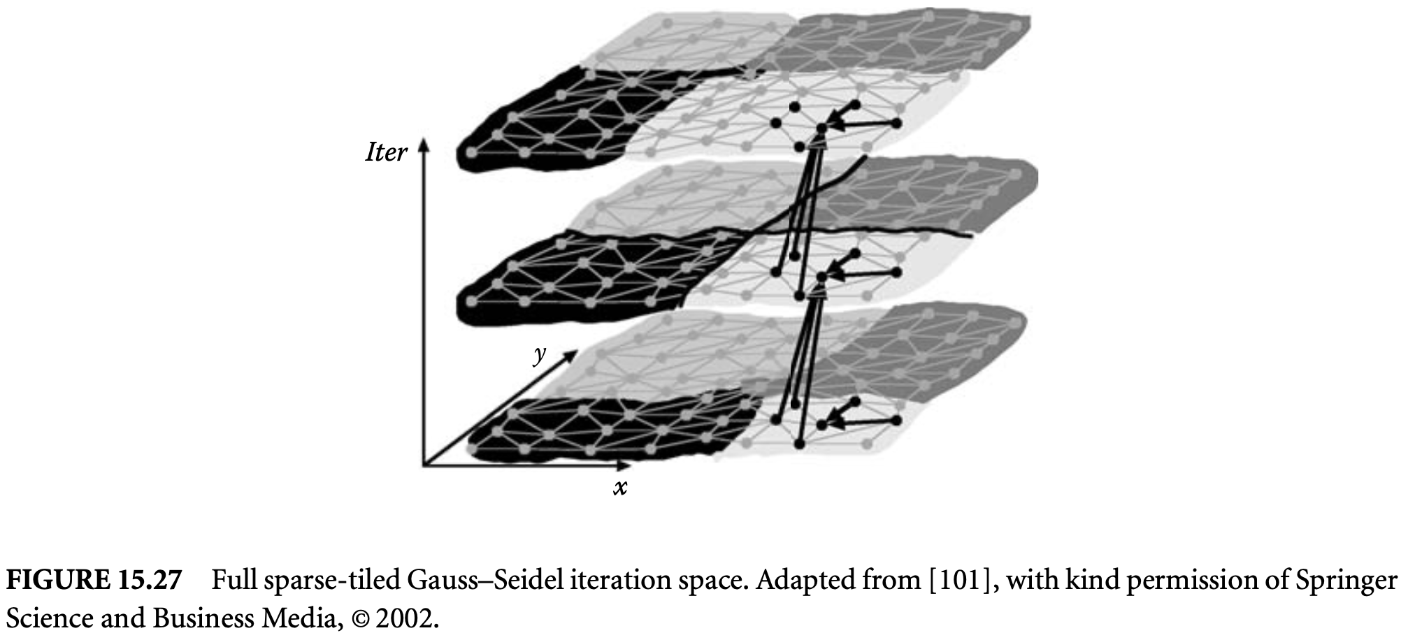
order, , given to the unknowns and corresponding matrix rows and columns is often arbitrary and can be changed without affecting the convergence properties of Gauss-Seidel. Therefore, if the unknowns are mapped to another order before performing Gauss-Seidel, the final numerical result will vary somewhat, but the convergence properties still hold.
In linear Gauss-Seidel, the data dependences arise from the nonzero structure of the sparse matrix . Each iteration point depends on the iteration points of its neighbors in the matrix graph from either the current or the previous convergence iteration, depending on whether the neighbor's index is ordered before or after . The dependences between iteration points within the same convergence iteration make parallelization of Gauss-Seidel especially difficult. Approaches to parallelizing Gauss-Seidel that maintain the same pattern of Gauss-Seidel data dependences use the fact that it is possible to apply an a priori reordering to the unknowns and the corresponding rows of the sparse matrix . This domain-specific knowledge is impossible to analyze with a compiler, so while automating full sparse tiling, it is necessary to provide some mechanism for a domain expert to communicate such information to the program analysis tool.
Figure 15.27 illustrates how the full sparse tiling inspector divides the Gauss-Seidel iteration space into tiles. The process starts by performing a seed partitioning on the matrix graph. In Figure 15.27, the seed-partitioned matrix graph logically sits at the second convergence iteration, and tiles are grown to the first and third convergence iterations.14 The tile growth must satisfy the dependences. For Gauss-Seidel, that involves creating and maintaining a new data order during tile growth. The full sparse tiling executor is a transformed version of the original Gauss-Seidel computation that executes each tile atomically (see Figure 15.28).
Footnote 14: The number of iterations for tile growth is usually small (i.e., two to five), and the full sparse tiling pattern can be repeated multiple times if necessary. The tile growth is started from a middle iteration to keep the size of the tiles as small as possible.
At runtime, the full sparse tiling inspector generates a data reordering function for reordering the rows and columns in the matrix, , and a tiling function, x . The tiling function maps iteration points to tiles. From this tiling function, the inspector creates a schedule function, x . The schedule function specifies for each tile and convergence iteration the subset of the reordered unknowns that must be updated. The transformed code shown in Figure 15.28 performs a tile-by-tile execution of the iteration points using the schedule function, which is created by the inspector to satisfy the following:

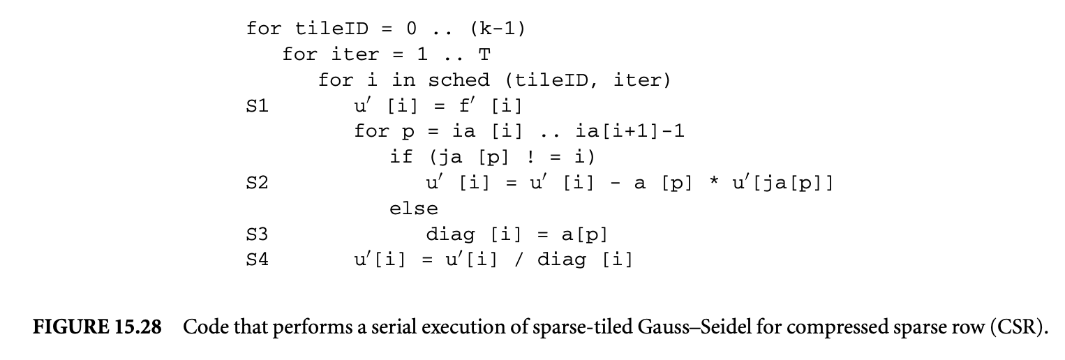
A matrix graph partitioning serves as a seed partitioning from which tiles can be grown. The seed partitioning determines the tiling at a particular convergence iteration, . Specifically at , where , the tiling function is set to the partition function, . To determine the tiling at other convergence iterations, the tile growth algorithm adds or deletes nodes from the seed partition as needed to ensure that atomic execution of each tile does not violate any data dependences.
The FullSparseNaive_GSCSR algorithm, shown in Figure 15.29, generates the tiling function for the Gauss-Seidel computation in Figure 15.25. While generating the tiling function, ordering constraints between nodes in the matrix graph are maintained in the relation NodeOrd. The first two statements in
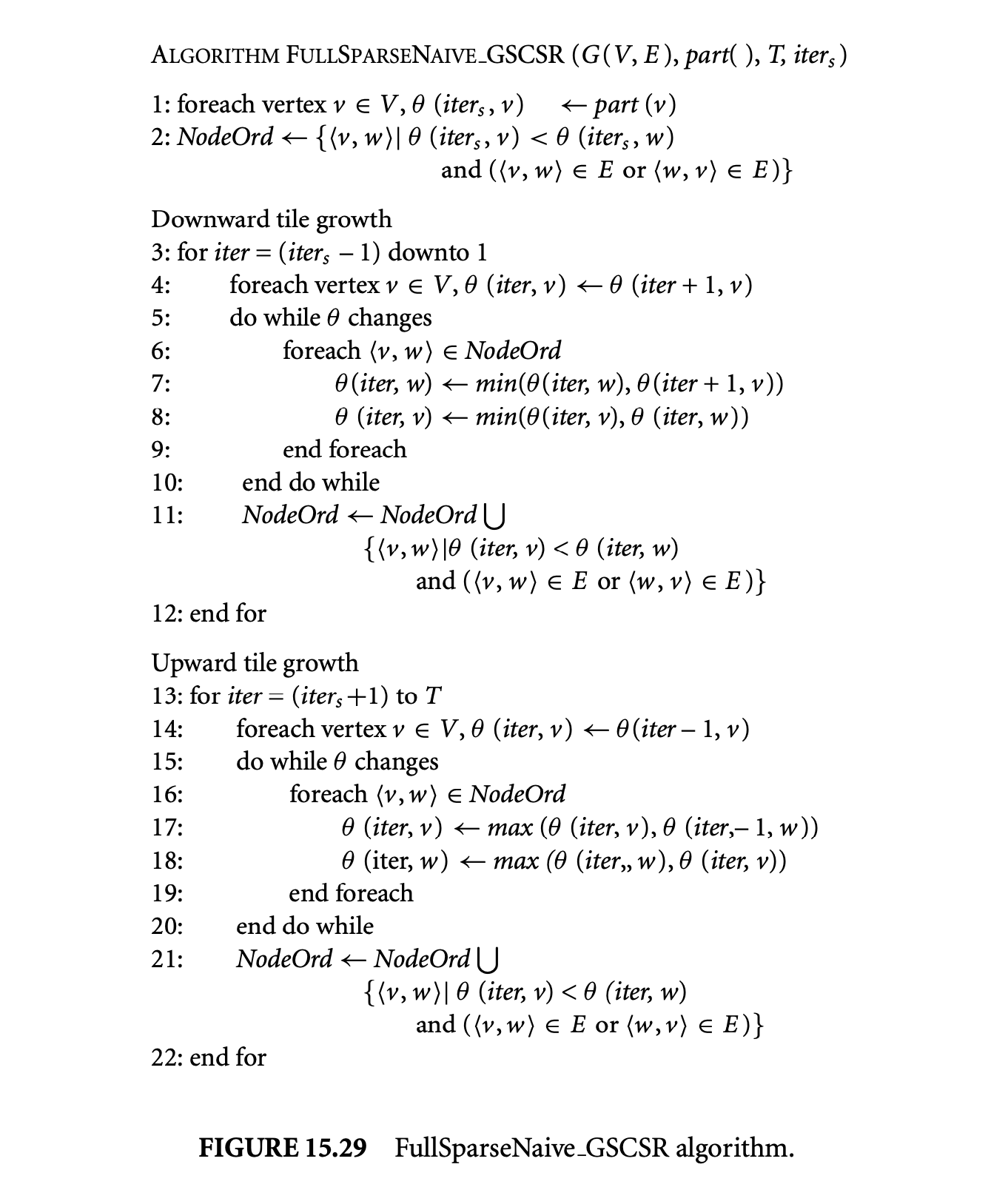 the algorithm initialize the NodeOrd relation and all of the tiling function values for the convergence iteration . The algorithm then loops through the convergence iterations such that , setting at each iteration point to . Finally, it visits the edges that have endpoints in two different partition cells, adjusting the tiling function to ensure that the data dependences are satisfied. The process is repeated for the convergence iterations between and in the upward tile growth. Once neighboring nodes, , are put into two different tiles at any iteration , the relative order between these two nodes must be maintained. The NodeOrd relation maintains that relative order. For example, if , then .
The running time of this algorithm is , where is the number of convergence iterations, is the number of tiles, is the number of nodes in the matrix graph, and is the number of edges in the matrix graph. The term is due to the while loops that begin at lines 5 and 15. In the worst case, the while loop will execute times, with only one value decreasing (or increasing in the forward tile growth) each time through the while loop. Each can take on values between 1 and , where is the number of tiles. In practice, the algorithm runs much faster than this bound.
To exploit parallelism, the inspector creates a tile dependence graph, and the executor for the full sparse-tiled computation executes sets of independent tiles in parallel. The tile dependence graph is used by a master-worker implementation that is part of the executor. The master puts tiles whose data dependences are satisfied on a ready queue. The workers execute tiles from the ready queue and notify the master upon completion. The following is an outline of the full sparse tiling process for parallelism:
- Partition the matrix graph to create the seed partitioning.
- Choose a numbering on the cells of the seed partition. The numbering dictates the order in which tiles are grown and affects the resulting parallelism in the tile dependence graph (TDG). A numbering that is based on a coloring of a partition interaction graph results in much improved TDG parallelism.
- Grow tiles from each cell of the seed partitioning in turn, based on the numbering, to create the tiling function that assigns each iteration point to a tile. The tile growth algorithm will also generate constraints on the data reordering function.
- Reorder the data using a reordering function that satisfies the constraints generated during tile growth.
- Reschedule by creating a schedule function based on the tiling function . The schedule function provides a list of iteration points to execute for each tile at each convergence iteration.
- Generate a TDG identifying which tiles may be executed in parallel.
15.3.3 Bibliographic Notes
As early as 1969, McKellar and Coffman [71] studied how to match the organization of matrices and their operations to paged memory systems. Early studies of such matching, in the context of program transformation, were done by Abu-Sufah et al. [2] and Wolfe and coworkers [55, 109]. Irigoin and Triolet [49] in their seminal work give validity conditions for arbitrary parallelepiped tiling. These conditions were further refined by Xue [113].
Tiling for memory hierarchy is a well-studied problem, and so is the problem of modeling the cache behavior of a loop nest. Several analytical models measure the number of cache misses for a given class of loop nests. These models can be classified into precise models that use sophisticated (computationally costly) methods and approximate models that provide a closed form with simple analysis. In the precise category, we have the cache miss equations [40] and the refinement by Chatterjee et al. [17], which use Ehrhart polynomials [18] and Presburger formulae to describe the number of cache misses. Harper et al. [44] propose an analytical model of set-associative caches and Cascaval and Padua [15] give a compile-time technique to estimate cache misses using stack distances. In the approximate category, Ferrante et al. [34] present techniques to estimate the number of distinct cache lines touched by a given loop nest.
Sarkar [94] presents a refinement of this model. Although the precise models can be used for selecting the optimal tile sizes, only Abella et al. [1] have proposed a near-optimal loop tiling using cache miss equations and genetic algorithms. Sarkar and Megiddo [95] have proposed an algorithm that uses an approximate model [34] and finds the optimal tile sizes for loops of depth up to three.
Several algorithms [16, 19, 47, 54] have been proposed for single-level tile size selection (see Hsu and Kremer [47] for a good comparison). The majority of them use an indirect cost function such as the number of capacity misses or conflict misses, and not a direct metric such as overall execution time. Mitchell et al. [74] illustrate how such local cost functions may not lead to globally optimal performance.
Mitchell et al. [74] were the first to quantify the multilevel interactions of tiling. They clearly point out the importance of using a global metric such as execution time rather than local metrics such as number of misses. Furthermore, they also show, through examples, the interactions between different levels of tiling and hence the need for a framework in which the tile sizes at all the levels are chosen simultaneously with respect to a global cost function. Other results that show the application and importance of multilevel tiling include [14, 50, 75]. Auto-tuners such as PHiPHAC [12] and ATLAS [106] use a model-driven empirical approach to choose the optimal tile sizes.
The description of optimal tiling literature presented above and the GP-based approach presented in this chapter is based on the work of Renganarayanan and Rajopadhye [91]12, who present a general technique for optimal multilevel tiling of rectangular iteration spaces with uniform dependences. YALMIP [68] is a tool that provides a symbolic interface to many optimization solvers. In particular, it provides an interface for defining and solving IGPs.
Portions reprinted, with permission, from [91], © 2004 IEEE.
15.3.3.1 Tiled Loop Generation13
16: Parts of this section are based on [92], © 2007, Association for Computing Machinery, Inc., included with permission.
Ancourt and Irigoin proposed a technique [6] for scanning a single polyhedron, based on Fourier-Motzkin elimination over inequality constraints. Le Verge et al. [61] proposed an algorithm that exploits the dual representation of polyhedra with vertices and rays in addition to constraints. The general code generation problem for affine control loops requires scanning unions of polyhedra. Kelley et al. [53] solved this by extending the Ancourt-Irigoin technique, and together with a number of sophisticated optimizations, developed the widely distributed Omega library [78]. The SUIF [108] tool has a similar algorithm. Quillere et al. proposed a dual-representation algorithm [80] for scanning the union of polyhedra, and this algorithm is implemented in the CLooG code generator [11] and its derivative Wloop used in the WRaP-IT project.
Code generation for fixed tile sizes can also benefit from the above techniques, thanks to Irigoin and Triolet's proof that the tiled iteration space is a polyhedron if the tile sizes are constants [49]. Either of the above tools may be used (in fact, most of them can generate such tiled code). However, it is well known that since the worst-case complexity of Fourier-Motzkin elimination is doubly exponential in the number of dimensions, this may be inefficient. Goumas et al. [41] decompose the generation into two subproblems, one to scan the tile origins, and the other to scan points within a tile, thus obtaining significant reduction of the worst-case complexity. They propose a technique to generate code for fixed-sized, parallelogram tiles.
There has been relatively little work for the case when tile sizes are symbolic parameters, except for the very simple case of orthogonal tiling: either rectangular loops tiled with rectangular tiles or loops that can be easily transformed to this. For the more general case, the standard solution, as described in Xue's text [114], has been to simply extend the iteration space to a rectangular one (i.e., to consider its bounding box) and apply the orthogonal technique with appropriate guards to avoid computations outside the original iteration space.
Amarasinghe and Lam [4, 5] implemented, in the SUIF tool set, a version of Fourier-Motzkin Elimination (FME) that can deal with a limited class of symbolic coefficients (parameters and block sizes), but the full details have not been made available. Grosslinger et al. [42] have proposed an extension to the polyhedral model, in which they allow arbitrary rational polynomials as coefficients in the linear constraints that define the iteration space. Their generosity comes at the price of requiring computationally very expensive machinery such as quantifier elimination in polynomials over the real algebra to simplify constraints that arise during loop generations. Because of this their method does not scale with the number of dimensions and the number of nonlinear parameters.
Jimenez et al. [51] develop code generation techniques for register tiling of nonrectangular iteration spaces. They generate code that traverses the bounding box of the tile iteration space to enable parameterized tile sizes. They apply index-set splitting to tiled code to traverse parts of the tile space that include only full tiles. Their approach involves less overhead in the loop nest that visits the full tiles; however, the resulting code experiences significant code expansion.
15.3.3.2 Tiling for Parallelism
Communication-minimal tiling refers to the problem of choosing the tile sizes such that the communication volume is minimized. Schriber and Dongarra [96] are perhaps the first to study communication-minimal tilings. Boulet et al. [13] are the first to solve the communication-minimal tiling optimally. Xue [112] gives a detailed comparison of various communication-minimal tilings.
Hogstedt et al. [45] studied the idle time associated with parallelepiped tiling. They characterize the time processor's wait for data from other processors. Desprez et al. [27] present simpler proofs to the solution presented by Hogstedt et al.
Several researchers [115, 46, 76, 86] have studied the problem of picking the tile sizes that minimize the parallel execution time. Andonov et al. [8, 7] have proposed optimal tile size selection algorithms for -dimensional rectangular and two-dimensional parallelogram iteration spaces. Our formulation of the optimal tiling problem for parallelism is very similar to theirs. They derive closed-form optimal solutions for both cases. We presented a GP-based framework that can be used to solve their formulation directly. Xue [114] gives a good overview of loop tiling for parallelism.
15.3.3.3 Tiling for Sparse Computations
Irregular memory references are also prevalent in popular games such as Unreal, which was analyzed as having 90% of its integer variables within index arrays such as B[103].
In Section 15.3.2.2, the static analysis techniques described were developed by Lin and Padua [65]. Pugh and Wonnacott [77] and Rus et al. [92] have developed techniques for extending static data dependence analysis with runtime checks, as discussed in Section 15.3.2.2. In [77] constraints for disproving dependences are generated at compile time, with the possibility of evaluating such constraints at runtime. Rus et al. [92] developed an interprocedural hybrid (static and dynamic) analysis framework, where it is possible to disprove all data dependences at runtime, if necessary.
Examples of runtime reordering transformation for data locality include [3, 20, 24, 28, 35, 43, 48, 72, 73, 99]. The pointer update optimization was presented by Ding and Kennedy [28].
Saltz et al. [93] originally developed inspector-executor strategies for the parallelization of irregular programs. Initially such transformations were incorporated into applications manually for parallelism [24]. Next, libraries with runtime transformation primitives were developed so that a programmer or compiler could insert calls to such primitives [25, 98].
Rauchwerger [88] surveys various techniques for dynamically scheduling iterations into wavefronts such that all of the iterations within one wavefront may be executed in parallel. Rauchwerger also discusses many issues such as load balancing, parallelizing the inspector, finding the optimal schedule, and removing anti and output dependences.
Strout et al. developed full sparse tiling [100, 101, 102]. Cache blocking of unstructured grids is another sparse tiling transformation, which was developed by Douglas et al. [29]. Wu [110] shows that reordering the unknowns in Gauss-Seidel does not affect the convergence properties.
References
[1] J. Abella, A. Gonzalez, J. Llosa, and X. Vera. 2002. Near-optimal loop tiling by mean of cache miss equations and genetic algorithms. In Proceedings of International Conference on Parallel Processing Workshops.
[2] W. Abu-Sufah, D. Kuck, and D. Lawrie. 1981. On the performance enhanceemmt of paging systems through program analysis and transformations. IEEE Trans. Comput. 30(5):341-56. [3] I. Al-Furaih and S. Ranka. 1998. Memory hierarchy management for iterative graph structures. In Proceedings of the 1st Merged International Parallel Processing Symposium and Symposium on Parallel and Distributed Processing, 298-302. [4] S. P. Amarasinghe. 1997. Parallelizing compiler techniques based on linear inequalities. PhD thesis, Computer Science Department, Stanford University, Stanford, CA. [5] Saman P. Amarasinghe and Monica S. Lam. 1993. Communication optimization and code generation for distributed memory machines. In PLDI '93: Proceedings of the ACM SIGPLAN 1993 Conference on Programming Language Design and Implementation, 126-38. New York: ACM Press. [6] C. Ancourt. 1991. Generation automatique de codes de transfert pour multiprocesseurs a memoires locales. PhD thesis, Universite de Paris VI. [7] Rumen Andonov, Stephan Balev, Sanjay V. Rajopadhye, and Nicola Yanev. 2003. Optimal semi-oblique tiling. IEEE Trans. Parallel Distrib. Syst. 14(9):944-60. [8] Rumen Andonov, Sanjay V. Rajopadhye, and Nicola Yanev. 1998. Optimal orthogonal tiling. In Euro-Par, 480-90. [9] C. Bastoul. 2002. Generating loops for scanning polyhedra. Technical Report 2002/23, PRiSM, Versailles University. [10] C. Bastoul, A. Cohen, A. Girbal, S. Sharma, and O. Temam. 2000. Putting polyhedral loop transformations to work. In Languages and compilers for parallel computers, 209-25. [11] Cedric Bastoul. 2004. Code generation in the polyhedral model is easier than you think. In IEEE PACT, 7-16. [12] Jeff Bilmes, Krste Asanovic, Chee-Whye Chin, and Jim Demmel. 1997. Optimizing matrix multiply using phipac: A portable, high-performance, ANSI C coding methodology. In Proceedings of the 11th International Conference on Supercomputing, 340-47. New York: ACM Press. [13] Pierre Boulet, Alain Darte, Tanguy Risset, and Yves Robert. (Pen)-ultimate tiling? Integr. VLSI J. 17(1):33-51. [14] L. Carter, J. Ferrante, F. Hummel, B. Alpern, and K. S. Gatlin. 1996. Hierarchical tiling: A methodology for high performance. Technical Report CS96-508, University of California at San Diego. [15] Calin Cascaval and David A. Padua. 2003. Estimating cache misses and locality using stack distances. In Proceedings of the 17th Annual International Conference on Supercomputing, 150-59. New York: ACM Press. [16] Jacqueline Chame and Sungdo Moon. 1999. A tile selection algorithm for data locality and cache interference. In Proceedings of the 13th International Conference on Supercomputing, 492-99. New York: ACM Press. [17] Siddhartha Chatterjee, Erin Parker, Philip J. Hanlon, and Alvin R. Lebeck. 2001. Exact analysis of the cache behavior of nested loops. In Proceedings of the ACM SIGPLAN 2001 Conference on Programming Language Design and Implementation, 286-97. New York: ACM Press. [18] Philippe Clauss. 1996. Counting solutions to linear and nonlinear constraints through Ehrhart polynomials: Applications to analyze and transform scientific programs. In Proceedings of the 10th International Conference on Supercomputing, 278-85. New York: ACM Press. [19] Stephanie Coleman and Kathryn S. McKinley. 1995. Tile size selection using cache organization and data layout. In Proceedings of the ACM SIGPLAN 1995 Conference on Programming Language Design and Implementation, 279-90. New York: ACM Press. [20] E. Cuthill and J. McKee. 1969. Reducing the bandwidth of sparse symmetric matrices. In Proceedings of the 24th National Conference ACM, 157-72. [21] A. Darte, Y. Robert, and F. Vivien. 2000. Scheduling and automatic parallelization. Basel, Switzerland: Birkhauser. [22] A. Darte, R. Schreiber, and G. Villard. 2005. Lattice-based memory allocation. IEEE Trans. Comput. 54(10):1242-57.
[23] Alain Darte and Yves Robert. 1995. Affine-by-statement scheduling of uniform and affine loop nests over parametric. J. Parallel Distrib. Comput. 29(1):43-59. [24] R. Das, D. Mavriplis, J. Saltz, S. Gupta, and R. Ponnusamy. 1992. The design and implementation of a parallel unstructured Euler solver using software primitives. AIAA J. 32:489-96. [25] R. Das, M. Uysal, J. Saltz, and Yuan-Shin S. Hwang. 1994. Communication optimizations for irregular scientific computations on distributed memory architectures. J. Parallel Distrib. Comput. 22(3):462-78. [26] E. De Greef, F. Catthoor, and H. De Man. 1997. Memory size reduction through storage order optimization for embedded parallel multimedia applications. In Parallel processing and multimedia. Geneva, Switzerland. Amsterdam, Netherlands: Elsevier Science. [27] Frederic Desprez, Jack Dongarra, Fabrice Rastello, and Yves Robert. 1997. Determining the idle time of a tiling: New results. In PACT '97: Proceedings of the 1997 International Conference on Parallel Architectures and Compilation Techniques, 307. Washington, DC: IEEE Computer Society. [28] C. Ding and K. Kennedy. 1999. Improving cache performance in dynamic applications through data and computation reorganization at run time. In Proceedings of the 1999 ACM SIGPLAN Conference on Programming Language Design and Implementation (PLDI), 229-41. New York: ACM Press. [29] C. C. Douglas, J. Hu, M. Kowarschik, U. Rude, and C. Weiss. 2000. Cache optimization for structured and unstructured grid multigrid. Electron. Trans. Numerical Anal. 10:21-40. [30] P. Feautrier. 1991. Dataflow analysis of array and scalar references. Int. J. Parallel Program. 20(1):23-53. [31] P. Feautrier. 1992. Some efficient solutions to the affine scheduling problem. Part I. One-dimensional time. Int. J. Parallel Program. 21(5):313-48. [32] P. Feautrier. 1992. Some efficient solutions to the affine scheduling problem. Part II. Multidimensional time. Int. J. Parallel Program. 21(6):389-420. [33] Agustin Fernandez, Jose M. ILaberia, and Miguel Valero-Garcia. 1995. Loop transformation using nonunimodular matrices. IEEE Trans. Parallel Distrib. Syst. 6(8):832-40. [34] J. Ferrante, V. Sarkar, and W. Thrash. 1991. On estimating and enhancing cache effectiveness. In Fourth International Workshop on Languages and Compilers for Parallel Computing, ed. U. Banerjee, D. Gelernter, A. Nicolau, and D. Padua, 328-43. Vol. 589 of Lecture Notes on Computer Science. Heidelberg, Germany: Springer-Verlag. [35] Jinghua Fu, Alex Pothen, Dimitri Mavriplis, and Shengnian Ye. 2001. On the memory system performance of sparse algorithms. In Eighth International Workshop on Solving Irregularly Structured Problems in Parallel. [36] Gautam, DaeGon Kim, and S. Rajopadhye. Scheduling in the -polyhedral model. In Proceedings of the IEEE International Symposium on Parallel and Distributed Systems (Long Beach, CA, USA, March 26-30, 2007). IPDPS '07. IEEE Press, 1-10. [37] Gautam and S. Rajopadhye. 2007. The -polyhedral model. PPoPP 2007: ACM Symposium on Principles and Practice of Parallel Programming. In Proceedings of the 12th ACM SIGPLAN Symposium on Principles and Practice of Parallel Programming (San Jose, CA, USA, March 14-17, 2007). PPoPP '07. New York, NY: ACM Press, 237-248. [38] Gautam and S. Rajopadhye. 2006. Simplifying reductions. In POPL '06: Symposium on Principles of Programming Languages, 30-41. New York: ACM Press. [39] Gautam, S. Rajopadhye, and P. Quinton. 2002. Scheduling reductions on realistic machines. In SPAA '02: Symposium on Parallel Algorithms and Architectures, 117-26. [40] Somnath Ghosh, Margaret Martonosi, and Sharad Malik. 1999. Cache miss equations: A compiler framework for analyzing and tuning memory behavior. ACM Trans. Program. Lang. Syst. 21(4):703-46. [41] Georgios Goumas, Maria Athanasaki, and Nectarios Koziris. 2003. An efficient code generation technique for tiled iteration spaces. IEEE Trans. Parallel Distrib. Syst. 14(10):1021-34. [42] Armin Grosslinger, Martin Griebl, and Christian Lengauer. 2004. Introducing non-linear parameters to the polyhedron model. In Proceedings of the 11th Workshop on Compilers for Parallel Computers(CPC 2004), ed. Michael Gerndt and Edmond Kereku, 1-12. Research Report Series. LRR-TUM, Technische Universitat Munchen. [43] H. Han and C. Tseng. 2000. A comparison of locality transformations for irregular codes. In Proceedings of the 5th International Workshop on Languages, Compilers, and Run-time Systems for Scalable Computers. Vol. 1915 of Lecture Notes in Computer Science. Heidelberg, Germany: Springer. [44] John S. Harper, Darren J. Kerbyson, and Graham R. Nudd. 1999. Analytical modeling of set-associative cache behavior. IEEE Trans. Comput. 48(10):1009-24. [45] Karin Hogstedt, Larry Carter, and Jeanne Ferrante. 1997. Determining the idle time of a tiling. In POPL '97: Proceedings of the 24th ACM SIGPLAN-SIGACT Symposium on Principles of Programming Languages, 160-73. New York: ACM Press. [46] Karin Hogstedt, Larry Carter, and Jeanne Ferrante. 2003. On the parallel execution time of tiled loops. IEEE Trans. Parallel Distrib. Syst. 14(3):307-21. [47] C. Hsu and U. Kremer. 1999. Tile selection algorithms and their performance models. Technical Report DCS-TR-401, Computer Science Department, Rutgers University, New Brunswick, NJ. [48] E. Im and K. Yelick. 2001. Optimizing sparse matrix computations for register reuse in sparsity. In Computational Science -- ICCS 2001, ed. V. N. Alexandrov, J. J. Dongarra, B. A. Juliano, R. S. Renner, and C. J. K. Tan, 127-36. Vol. 2073 of Lecture Notes in Computer Science. Heidelberg, Germany: Springer-Verlag. [49] F. Irigoin and R. Triolet. 1988. Supernode partitioning. In 15th ACM Symposium on Principles of Programming Languages, 319-28. New York: ACM Press. [50] M. Jimenez, J. M. Liberia, and A. Fernandez. 2003. A cost-effective implementation of multilevel tiling. IEEE Trans. Parallel Distrib. Comput. 14(10):1006-20. [51] Marta Jimenez, Jose M. Liberia, and Agustin Fernandez. 2002. Register tiling in nonrectangular iteration spaces. ACM Trans. Program. Lang. Syst. 24(4):409-53. [52] R. M. Karp, R. E. Miller, and S. V. Winograd. 1967. The organization of computations for uniform recurrence equations. J. ACM 14(3):563-90. [53] W. Kelly, W. Pugh, and E. Rosser. 1995. Code generation for multiple mappings. In Frontiers '95: The 5th Symposium on the Frontiers of Massively Parallel Computation. [54] Monica D. Lam, Edward E. Rothberg, and Michael E. Wolf. 1991. The cache performance and optimizations of blocked algorithms. In Proceedings of the Fourth International Conference on Architectural Support for Programming Languages and Operating Systems, 63-74. New York: ACM Press. [55] Monica S. Lam and Michael E. Wolf. 1991. A data locality optimizing algorithm (with retrospective). In Best of PLDI, 442-59. [56] Leslie Lamport. 1974. The parallel execution of DO loops. Commun. ACM 17(2) 83-93. [57] V. Lefebvre and P. Feautrier. 1997. Optimizing storage size for static control programs in automatic parallelizers. In Euro-Par'97, ed. C. Lengauer, M. Griebl, and S. Gorlatch. Vol. 1300 of Lecture Notes in Computer Science. Heidelberg, Germany: Springer-Verlag. [58] P. Lenders and S. V. Rajopadhye. 1994. Multirate VLSI arrays and their synthesis. Technical Report 94-70-01, Oregon State University. [59] H. Le Verge. 1992. Un environment de transformations de programmes pour la synthese d'architectures regulieres. PhD thesis, L'Universite de Rennes I, IRISA, Campus de Beaulieu, Rennes, France. [60] H. Le Verge. 1995. Recurrences on lattice polyhedra and their applications. Based on a manuscript written by H. Le Verge just before his untimely death. [61] H. Le Verge, V. Van Dongen, and D. Wilde. 1994. Loop nest synthesis using the polyhedral library. Technical Report PI 830, IRISA, Rennes, France. Also published as INRIA Research Report 2288. [62] Wei Li and Keshav Pingali. 1994. A singular loop transformation framework based on non-singular matrices. Int. J. Parallel Program. 22(2):183-205. [63] Amy W. Lim, Gerald I. Cheong, and Monica S. Lam. 1999. An affine partitioning algorithm to maximize parallelism and minimize communication. In International Conference on Supercomputing, 228-37.
[64] Amy W. Lim, Shih-Wei Liao, and Monica S. Lam. 2001. Blocking and array contraction across arbitrarily nested loops using affine partitioning. In PPoPP '01: Proceedings of the Eighth ACM SIGPLAN Symposium on Principles and Practices of Parallel Programming, 103-12. New York: ACM Press. [65] Yuan Lin and David Padua. 2000. Compiler analysis of irregular memory accesses. In Proceedings of the ACM SIGPLAN Conference on Programming Language Design and Implementation, 157-68. Vol. 35. [66] B. Lisper. 1990. Linear programming methods for minimizing execution time of indexed computations. In International Workshop on Compilers for Parallel Computers. [67] Yanhong A. Liu, Scott D. Stoller, Ning Li, and Tom Rothamel. 2005. Optimizing aggregate array computations in loops. ACM Trans. Program. Lang. Syst. 27(1):91-125. [68] J. Lofberg. 2004. YALMIP: A toolbox for modeling and optimization in MATLAB. In Proceedings of the CACSD Conference. http://control.ee.ethz.ch/~joloef/yalmip.php. [69] C. Mauras. 1989. ALPHA: Un langage equationnel pour la conception et la programmation d'architectures paralleles synchrones. PhD thesis, l'Universite de Rennes I, Rennes, France. [70] C. Mauras, P. Quinton, S. Rajopadhye, and Y. Saouter. 1990. Scheduling affine parametrized recurrences by means of variable dependent timing functions. In International Conference on Application Specific Array Processing, 100-10. [71] A. C. McKellar and E. G. Coffman, Jr. 1969. Organizing matrices and matrix operations for paged memory systems. Commun. ACM 12(3):153-65. [72] J. Mellor-Crummey, D. Whalley, and K. Kennedy. 1999. Improving memory hierarchy performance for irregular applications. In Proceedings of the 1999 ACM SIGARCH International Conference on Supercomputing (ICS), 425-33. [73] N. Mitchell, L. Carter, and J. Ferrante. 1999. Localizing non-affine array references. In Proceedings of the 1999 International Conference on Parallel Architectures and Compilation Techniques, 192-202. [74] N. Mitchell, N. Hogstedt, L. Carter, and J. Ferrante. 1998. Quantifying the multi-level nature of tiling interactions. Int. J. Parallel Program. 26(6):641-70. [75] Juan J. Navarro, Toni Juan, and Toms Lang. 1994. Mob forms: A class of multilevel block algorithms for dense linear algebra operations. In Proceedings of the 8th International Conference on Supercomputing, 354-63. New York: ACM Press. [76] Hiroshi Ohta, Yasuhiko Saito, Masahiro Kainaga, and Hiroyuki Ono. 1995. Optimal tile size adjustment in compiling general doacross loop nests. In ICS '95: Proceedings of the 9th International Conference on Supercomputing, 270-79. New York: ACM Press. [77] B. Pugh and D. Wonnacott. 1994. Nonlinear array dependence analysis. Technical Report CS-TR-3372, Department of Computer Science, University of Maryland, College Park. [78] W. Pugh. 1992. A practical algorithm for exact array dependence analysis. Commun. ACM 35(8):102-14. [79] Fabien Quillere and Sanjay Rajopadhye. 2000. Optimizing memory usage in the polyhedral model. ACM Trans. Program. Lang. Syst. 22(5):773-815. [80] Fabien Quillere, Sanjay Rajopadhye, and Doran Wilde. 2000. Generation of efficient nested loops from polyhedra. Int. J. Parallel Program. 28(5):469-98. [81] P. Quinton, S. Rajopadhye, and T. Risset. 1996. Extension of the alpha language to recurrences on sparse periodic domains. In ASAP '96, 391. [82] Patrice Quinton and Vincent Van Dongen. 1989. The mapping of linear recurrence equations on regular arrays. J. VLSI Signal Process. 1(2):95-113. [83] S. V. Rajopadhye, S. Purushothaman, and R. M. Fujimoto. 1986. On synthesizing systolic arrays from recurrence equations with linear dependencies. In Foundations of software technology and theoretical computer science, 488-503. [84] Easwaran Raman and David August. 2007. Optimizations for memory hierarchy. In The compiler design handbook: Optimization and machine code generation. Boca Raton, FL: CRC Press.
[85] J. Ramanujam. 1995. Beyond unimodular transformations. J. Supercomput. 9(4):365-89. [86] J. Ramanujam and P. Sadayappan. 1991. Tiling multidimensional iteration spaces for nonshared memory machines. In Supercomputing '91: Proceedings of the 1991 ACM/IEEE Conference on Supercomputing, 111-20. New York: ACM Press. [87] S. K. Rao. 1985. Regular iterative algorithms and their implementations on processor arrays. PhD thesis, Information Systems Laboratory, Stanford University, Stanford, CA. [88] Lawrence Rauchwerger. 1998. Run-time parallelization: Its time has come. Parallel Comput. 24(3-4):527-56. [89] Xavier Redon and Paul Feautrier. 1993. Detection of recurrences in sequential programs with loops. In PARLE '93: Parallel Architectures and Languages Europe, 132-45. [90] Xavier Redon and Paul Feautrier. 1994. Scheduling reductions. In International Conference on Supercomputing, 117-25. [91] Lakshminarayanan Renganarayana and Sanjay Rajopadhye. 2004. A geometric programming framework for optimal multi-level tiling. In SC '04: Proceedings of the 2004 ACM/IEEE Conference on Supercomputing, 18. Washington, DC: IEEE Computer Society. [92] S. Rus, L. Rauchwerger, and J. Hoeflinger. 2002. Hybrid analysis: Static & dynamic memory reference analysis. In Proceedings of the 16th Annual ACM International Conference on Supercomputing (ICS). [93] Joel H. Salz, Ravi Mirchandaney, and Kay Crowley. 1991. Run-time parallelization and scheduling of loops. IEEE Trans. Comput. 40(5):603-12. [94] V. Sarkar. 1997. Automatic selection of high-order transformations in the IBM XL Fortran compilers. IBM J. Res. Dev. 41(3):233-64. [95] V. Sarkar and N. Megiddo. 2000. An analytical model for loop tiling and its solution. In Proceedings of ISPASS. [96] R. Schreiber and J. Dongarra. 1990. Automatic blocking of nested loops. Technical Report 90.38, RIACS, NASA Ames Research Center, Moffett Field, CA. [97] W. Shang and J. Fortes. 1991. Time optimal linear schedules for algorithms with uniform dependencies. IEEE Trans. Comput. 40(6):723-42. [98] Shamik D. Sharma, Ravi Ponnusamy, Bongki Moon, Yuan-Shin Hwang, Raja Das, and Joel Sultz. 1994. Run-time and compile-time support for adaptive irregular problems. In Supercomputing '94. Washington, DC: IEEE Computer Society. [99] J. P. Singh, C. Holt, T. Totsuka, A. Gupta, and J. Hennessy. 1995. Load balancing and data locality in adaptive hierarchical -body methods: Barnes-Hut, fast multipole, and radiosity. J. Parallel Distrib. Comput. 27(2):118-41. [100] M. M. Strout, L. Carter, and J. Ferrante. 2001. Rescheduling for locality in sparse matrix computations. In Computational Science -- ICCS 2001, ed. V. N. Alexandrov, J. J. Dongarra, B. A. Juliano, R. S. Renner, and C. J. K. Tan. Vol. 2073 of Lecture Notes in Computer Science. Heidelberg, Germany: Springer-Verlag. [101] M. M. Strout, L. Carter, J. Ferrante, J. Freeman, and B. Kraeseck. 2002. Combining performance aspects of irregular Gauss-Seidel via sparse tiling. In Proceedings of the 15th Workshop on Languages and Compilers for Parallel Computing (LCPC). [102] Michelle Mills Strout, Larry Carter, and Jeanne Ferrante. 2003. Compile-time composition of runtime data and iteration reorderings. In Proceedings of the 2003 ACM SIGPLAN Conference on Programming Language Design and Implementation (PLDI). [103] Tim Sweeney. 2006. The next mainstream programming language: A game developer's perspective. Invited talk at ACM SIGPLAN Conference on Principles of Programming Languages (POPL). Charleston, SC, USA. [104] J. Teich and L. Thiele. 1993. Partitioning of processor arrays: A piecewise regular approach. INTERGRATION: VLSI J. 14(3):297-332. [105] William Thies, Frederic Vivien, Jeffrey Sheldon, and Saman P. Amarasinghe. 2001. A unified framework for schedule and storage optimization. In Proceedings of the 2001 ACM SIGPLAN Conference on Programming Language Design and Implementation, 232-42, Snowbird, Utah, USA.
[106] R. Clint Whaley and Jack J. Dongarra. 1998. Automatically tuned linear algebra software. In Proceedings of the 1998 ACM/IEEE Conference on Supercomputing (CDROM), 1-27. Washington, DC: IEEE Computer Society. [107] D. Wilde. 1993. A library for doing polyhedral operations. Technical Report PI 785, IRISA, Rennes, France. [108] R. P. Wilson, Robert S. French, Christopher S. Wilson, S. P. Amarasinghe, J. M. Anderson, S. W. K. Tjiang, S.-W. Liao, C.-W. Tseng, M. W. Hall, M. S. Lam, and J. L. Hennessy. 1994. SUIF: An infrastructure for research on parallelizing and optimizing compilers. SIGPLAN Notices 29(12):31-37. [109] Michael Wolfe. 1989. Iteration space tiling for memory hierarchies. In Proceedings of the Third SIAM Conference on Parallel Processing for Scientific Computing, 357-61, Philadelphia, PA: Society for Industrial and Applied Mathematics. [110] C. H. Wu. 1990. A multicolour SOR method for the finite-element method. J. Comput. Applied Math. 30(3):283-94. [111] Jingling Xue. 1994. Automating non-unimodular loop transformations for massive parallelism. Parallel Comput. 20(5):711-28. [112] Jingling Xue. 1997. Communication-minimal tiling of uniform dependence loops. J. Parallel Distrib. Comput. 42(1):42-59. [113] Jingling Xue. 1997. On tiling as a loop transformation. Parallel Process. Lett. 7(4):409-24. [114] Jingling Xue. 2000. Loop tiling for parallelism. Dordrecht, The Netherlands: Kluwer Academic Publishers. [115] Jingling Xue and Wentong Cai. 2002. Time-minimal tiling when rise is larger than zero. Parallel Comput. 28(6):915-39.